T ET {Xi}& be a stationary process (i.e., stationary. Fig. 1. General feedback quantization scheme ti information source) with values in the set a,. Suppose.
248
IEEE TRANSACTIONS
ON INFORMATION
THEORY,
IT-28, NO. 2, MARCH1982
VOL.
Stochastic Stability for Feedback Quantization Schemes JOHN C. RIEFFER
A hsfrucf -Feedback quantization schemes (such as delta modulation, adaptive quantization, differential pulse code modulation (DPCM), and adaptive differential pulse code modulation (ADPCM) encode an information source by quantizing the source letter at each time i using a quantizer, which is uniquely determined by examining some function of the past outputs and inputs called the state of the encoder at time i. The quantized output letter at time i is fed back to the encoder, which then moves to a new state at time i + I which is a function of the state at time i and the encoder output at time i. In an earlier paper a stochastic stability result was obtained for a class of feedback quantization schemeswhich includes delta modulation and some adaptive quantization schemes.In this paper a similar result ‘is obtained for a class of feedback quantization schemes which includes linear DPCM and some ADPCM encoding ‘schemes. The type of stochastic stability obtained gives almost-sure convergence of time averages of functions of the joint input-state-output process. This is stronger than the type of stochastic stability obtained previously by Gersho, Goodman, Goldstein, and Liu, who showed convergence in. distribution of the time i input-state-output as i + .03.
I.
INTRODUCTION
Xl
Q
>
>
2,
G
s ItI
Fig. 1. General feedback quantization scheme
T ET {Xi}& be a stationary process (i.e., stationary ti information source) with values in the set a,. Suppose we wish to quantize {Xi} into a process { Z,}~?“,,with values in a finite set A. Feedback quantization schemesin common use in communication theory accomplish this in the following way. For every state s in a certain metric space Q2,,a quantizer Q, from L!, - A is given. If the encoder is in a given state S, E Q2,at time i, Xi is encoded into i 2 0. (1) Z, = Q&T), The encoder then moves to state S,, , at time i + 1 according to the formula
ferential pulse code modulation (DPCM), and adaptive differential pulse code modulation (ADPCM). Various types of stochastic stability results have been obtained for feedback quantization schemes.They all involve the asymptotic behavior of sequencesof averages {n-‘Z;z;f(qy zpo, SpO)};~,, for a certain class of functions f, where X,?’denotes (Xi, X,, 1, . . . ) and similarly for Zp, SpO.The first and weakest type of stochastic stability considered was that in which n-l
(2)
i L 0, s IS-1= G(Z,, a, where G is some function from A X 51, - &. In this way the input process {Xi}& is encoded into the quantizer output process {Zi}~& by means of the quantizer state process {Si}cO, the state of the encoder at each time being determined from the previous state and previous output (which constitutes feedback to the encoder). This encoding procedure is indicated schematically in Fig. 1. There are a wide variety of feedback quantization schemes, among which are delta modulation, adaptive quantization, dif-
n- ’ izo f( X, , Zi > si>
converges I
(3)
for every bounded continuous f. Delta modulation [l], a certain kind of adaptive quantization [5], and certain DPCM and ADPCM encoding schemes [4] were shown to exhibit this kind of stochastic stability. Recently a stronger type of stochastic stability was considered by Kieffer and Dunham [7]. They showed that for a class of feedback quantization schemes including delta modulation and many adaptive quantization schemes(but not DPCM or ADPCM) L-1 %’ E/ vm ;m cm
Manuscript received March 10, 1981; revised August 12, 1981. This work was supported by National Science Foundation under Grant ECS7821335. The author is with the Department of Mathematics and Statistics, University of Missouri, Rolla, MO 65401.
convergesalmost surely (4) )I as n + cc for every bounded measurablef. L J\“i i=O
9 by ) Oi
In this paper we obtain a type of stochastic stability for a
001%9448/82/0300-0248$00.75 01982 IEEE
KIEFFER:
STOCHASTIC
STABILITY
FOR FEEDBACK
QUANTIZATION
249
SCHEMES
class of feedback quantization schemesincluding linear Let C C at, be the countable set of states DPCM and someADPCM schemes.The type of stochastic C = {s*} U g(A*). stability obtained is stronger than (3) but not quite as strong as (4) in that the bounded measurablefunction f in If x E &I,, s E &, define (4) has to be required to be continuousin the third variable qs, x) = sup {S 2 0: s’ E C and d(s, s’) I 6 (the state variable). This is all m a d e precise in the next imply Q,(x) = Q&)). section where we state our m a in result. The number 6(s, x) is just the m o d u lus of continuity of Q , II. STATEMENTOFMAINRESULT at x. It is easy to show that the m a p (s, x) + 6(s, x) is a measurablem a p from a2, X a, + [0, co]. F ix for this section a standard measurablespacea, (see, Here is our m a in result. It is proved in the Appendix. e.g., [8]), a complete separablemetric spaceG2,with metric d (which we make into a measurablespacewhosemeasurable sets are the Bore1sets),a finite set A, a family of maps {Qs: s E ti2,} from &?,-+ A for which the m a p (s, x) + Q ,(x) from a2, X 9, + A is jointly measurable, and a measurablefunction G : A X Q2,+ 52,. W e call the maps {Q,} quantizers; we call G the state transition function. Let {Xi}~=o be an a,-valued process;i.e., a sequenceof measurablefunctions from some probability space to a,. This is the input source which we wish to encode. Let {Zi}~?o be the A-valued processand {S,}~?“=, the !&valued processgiven by
s, = s*, Z, = si+l
and for every i 2 0,
si>,
= G(z,,
b) there exists N > 0 and cu(0< (Y< 1) such that for every n L N, if z E A” and w E A, then
(5)
g(z) = G(z, s*>, . . A)
and
W e remark that assumptionb) is true if for each z E A, the m a p p ing G(z, -): ti2, + 52,is a contraction.
where s* is any fixed element of &?,. W e call {Zi} the quantizer output processand {Si} the quantizer state process. If !J is a measurablespacelet IJ(O,co) denote the product measurablespaceof all sequences(oa, w,, . . . ) from &I. If {q}& is an a-valued processlet UT denote the n(O, co)valued measurablefunction (U,, U,,‘, , . . . ). W e now define the type of stochastic stability to be considered in this paper. W e define the triple process {(Xi, Z,, S,)} to be stochastically stable if {n-‘Z;:;f(XiP”, ZF, Sim)} convergesalmost surely as n + cc for every boundedf: Q ,(O,co) X A(0, 00) X !&(O, 00) -+ (- 00, 00) for which f(x, z, e): Q2,(0,00)-+ (- 00, 00) is continuous for each x E a,(O, co), z E A(0, cc), and f(., ., s): a,(O, 00) X A(0, co) + (- co, co) is measurable for every s E ti2,(0,co). (Note: such a function f is jointly measurableon the product space ti,(O, co) X A(0, co) X $(O, cc); (seeL e m m a 2 of the Appendix). O n &!,(O,cc), we are placing the usual product topology.) The m a in result of this paper, (Theorem l), gives stochastic stability of the joint input-output-state process for a class of feedback quantization schemeswhich includes linear DPCM and someADPCM schemes. To state this result we need some more notation. Let A* = Urn n=,A”; A* is thus the set of all finite-length sequencesfrom A. Define a m a p g: A* -+ fJ2, so that
dz,,.
Pr[G(S,, Xi) I X] I MhP;
Then the process{(Xi, Z,, S,)} is stochasticallystable.
Q,,(4),
= G(Zi,
Theorem 1: Let {Xi}??=,be an O ,-valued stationary process.Let {Zi}Eo and {S,}T=*=, be the A-valued and O ,-valued processesgiven by (5). Supposethat a) there exists p > 0, M > 0, such ‘that for every i = 0,l; . . , and every x 1 0,
z EA;
g(z,>->z,-,)>, Z,,’ . .,z,, E A,
n 22.
In SectionIII we apply this theorem to linear DPCM. In Section IV it is applied to an ADPCM encoding scheme. III.
APPLICATIONTO DPCM
Let R denote the real line. F ix positive integersj, k, a vector a: = (a,; * *,a,) E Rk, a vector p = (R,; . .,Rk) E Rk, a quantizer Q : Rj -+ A C Rj (A finite), vectors td;, u:,; ’‘,ulik+, E Rj, and a stationary Rj-valued process {Xi)&. Define processes{Zi}FO, {q}zek+,, where u,=u;T,u-, =U;,**.,U-k+, =fPk+,, and for i 10, Zl =
Q( Xi
q+,
= z, + a,q
Theorem
- PIN - &q-I + a*q-,
-
. * * -Pk&k+,)>
+ . . . +akqpk+,.
(6)
2: {( 4, Z,, q)}F”=, is stochasticallystable if
1) for someM > 0, p > 0, and positive integer m, Pr{ Xi EEIX,;,Xii-,} I Mp(E)P almost surely for every i > m, and every Bore1subset E of Rj, where p denotesLebesguemeasureon Rj, 2) the roots of the polynomial xk - (Y,x~-’ - ... -(Ye all have m o d u lus less than one, 3) E[ll X0 II ‘1 < cc for some r > 0, where II . II denotes the Euclidean norm on Rj, and 4) the boundary of each atom Q-‘(a), a E A, is contained in the union of finitely many (j - l)dimensionalhyperplanes. Remarks: Assumption 1) is true, i.e., if {Xi} is a finitememory processwith each X, having a distribution absolutely continuous with respect to p, or if {Xi} is a nondeterministic GaussianInrocess.An examination of the nroof -~~- r- --
250
IEEE TRANSACTIONS
ON INFORMATION
THEORY,
VOL.
IT-28,
of Theorem 2, given at the end of this section, will show that assumption 3) can be dropped ifj = 1. Assumption 4) will hold if we map each x E Rj under Q into the closet point of A (which is a necessarycondition for optimality when the difference distortion measureis used [2]). With a lot more effort, it can be shown that assumption 4) can be weakened to the assumption that there are finitely many ( j - I)-dimensional manifolds M,, . . . ,M, such that the following conditions hold. a) The boundary of each Q-‘(a)
NO.
2,
MARCH
1982
$1
ui+1 V UNIT
is contained in M,
DELAY I
U *f* uhf,.
b) Each Mi is sufficiently smooth. c) Each Mi has finite surface area or else the surface area of Mi II B(r) does-not approach cc too fast as r + 00, where B(r) denotes the ball {x E Rj: IIxII
Fig. 2.
Differential
pulse code modulation.
5 r}.
We have not specified how smooth M, needs to be because this would take us too far afield in the theory of surface area. It seemseasier to duplicate the proof of Theorem 2 for the special type of manifold one encounters in a particular application, than it would be to give a proof of Theorem 2 valid for all manifolds. Example A: Let {Xi}EO be a real, stationary, nondeterministic, Gaussian process. Choose (Y,,(Ye,.. . , (Yeto be the optimum least-squarelinear prediction coefficients; i.e., choose them so that E[I X, - CY,X,-, - (Y*X~-~ - . . . -(Y~X;-~ 1’1is a minimum. It is well-known that (2) holds, [see 6, p. 401. Choose Q: R + A C R so that each Q-’ (a) is an interval. Choose (Y,= j3,; . a,(~~= pk. Code {X,} into {Z,} using {U,}, according to (6). This encoding schemeis linear DPCM, as catalogued in [3, fig. 1 and eq. (2)]. (Fig. 2 gives a block diagram depicting DPCM for k = 1.) From Theorem 2, we conclude that {(X., Z,, q)} is stochastically stable. Example B: Again let {Xi} be a real, stationary, nondeterministic Gaussian process. Let A > 0. Define Q: R -+ { -A, A} to be the quantizer x 20, Q(x) = A, = -A, x -=z0. Require that k = 1, /3 = 1 and 0 < (Y< 1. Code {X;} into {Z,} using {Ui}, according to (6). This encoding schemeis called delta modulation with “leaky” integration. Earlier Gersho [l] proved the weaker type of stochastic stability given by (3) for this encoding scheme. Proof
of
xk) E (Rj)k.
ifzER/andx=(x,;.., Zi =
Then, for i L 0,
Q,,(4),
and ‘i+1
=
G(Z,, S,).
Now {(Xi, Zj, q)} is stochastically stable if ((4, Z,, S,)} is. Therefore we complete the proof by showing that assumptions a) and b) of Theorem 1 hold, where on ( Rj)k we put the metric induced by the norm II(x,; . . ,xk)ll =[IIx,# L
+ ‘.’ +ilXkli2]“*.
First we demonstrate that a) of Theorem 1 holds. Fix > 0 so that lla * s - a . S’II 5 L/Is - s’ll,
s, s’ E (RJ)k.
Then, 6(s, x) 2 FlinL-‘d(x
- p * s, H),
for every s E ( Rj)k, x E Rj, where d denotes the Euclidean metric on Rj and X is a finite set of hyperplanes whose union contains the boundary of each Q-‘(u). For any i=O,l;*. and B > 0, and h 2 0, Pr[G(S,, X,) I h] SzPr[d(X, ,“,,
- p. Si, H) I LA]
E[llX,,I’]B-’ +~Pr[d(Xi-~~Si,H)~Lh,lIX,II
IB],
H
Theorem
2:
Let {S,}y=“=,be the (Ri)k-valued
process sj = (q,-J-k-t,),
i LO.
If y’= (y,; . . ,yk) E Rk and x = (x,; . .,xk) E (RJ)k, let y . x = y,x, + * . . +y,x,. For each s E (Rj)k, let Q,: Rj + RJ be the quantizer Q,(x) = Qb - P .s>. Let G: Ri X (R’)k G(z,(x,,-
+ ( Rj)k be the map ,x,)) = (z + a ’x, x,,“‘,xk-,),
where vertical bars ) . ( about a set are used to denote the number of elements in the set. Fix H E X. Now if i > m, where m is given by l), then S, is a function of X0, X,,...,Xi-m, ZI--m+,,...,Zj-, and so Pr[d(X,-a~&,H)ILA,lIX,II~B] 5
x
Pr[d(Xi-F,(X,,...,~-,>,H)
(7)
UEA”’
0, h > 0. Setting B = A-‘/J, the upper bound in (8) becomes ) X 1 E [II X0 II ‘]x’/j + 1 X ll A lrn M2pLp2p(j-‘)hp’j, whencea) of Theorem 1 is verified. W e now verify b) of Theorem 1. Let so* = (24;;. . ,uEk+,), and for each z E Rj, let T, be the m a p G(z, .) from (Rj)k + (Rj)k. Since each T, is a translation of the linear transformation T,, it is easily seenthat there is a constant M such that for each n and every choice z,, z2; . .,z,,+, E A, we have II&.
y
... .T,“)(S,*) - (rz, . Tz, . * . . .T,“+,)b,*)Il ‘M IITJI,
(9)
Theorem 3: Let c, = 0, c2 = 1 or c, = 1, c2 = 0. If the real, stationary process{Xi} satisfiescondition 1) of Theorem 2, then the joint process{(Xi, (Z,, A;), Si)}y?o is stochastically stable, where the processes{Z,), {hi}, {Si} are given by (10). Proof:
Define the B X R-valued process{g}n=o by s7,= (A,, s,J,
n 20.
Define the R*-valued process{X~}~o=oby n 20. x, = G L xn+A Let D be the fim te set U,,,Q,(R). Define the D X Bvalued process{Z,}c=o by
where IITo’II denotesthe norm of Ton, the norm used being the usual dual norm on the spaceof linear transformations n L 0. z, = (Zn> An+,), on ( Rj)k induced by the norm on ( Rj)k. W ith respectto a For each (A,s) E B X R, let &,: R* -D X B be the suitable basis for (RJ)k, it can be shown that the jk X jk matrix for To is a direct sum of j identical k X k matrices quantizer such that each of which has characteristicpolynomial xk - (Y,Xk-, e,, Sk x’> - . . . -1yk. Hence lim ,+, lITonII’/’ < 1 because of as= (Q,b - Ps), F,(c, Ix’ - b - PQ& - Ps) I sumption 2) of Theorem 2 and so assumptionb) of Theorem 1 follows from (9). +c, I x - at- - Q ,(x - Ps) I)). IV.
APPLICATIONTOAN ADPCM ENCODING SCHEME
Let B be a finite set and let c,, c2 be real numbers. For each A E B, let Q , be a step function from R + R and let F, be a step function from R + B. (If E is a set, we say that a function H: R + E is a step function if H(R) is finite and for each e E H(R), H-‘(e) is either an interval or a singleton.) F ix a number (YE R such that 0 < (Y< 1, and also fix /3 E R, so* E R, A: E B. Let {Xi}& be a real, stationary process which we quantize into the process {Z,}:‘“,, with the help of the processes{,Si}~o=o, {Ai}zo, according to the following adaptive quantization scheme with feedback So = s;, A, = A;, and for i 2 0, Z, = Q ,,(x, - Psi>, 4,’ = as, + z,, 4,’ = F ,t(clI x,+1- Psi+1 I +‘2 I X, - %+II>. (loI W e see that the adaptive quantization comes about by
Define G : (D X B) X (B X R) + B X R by G((z, A), (A’, s)) = (A, z + (YS). Then, for n 2 0, z, = e,;pJ,
and s,+, = G(Z,, s,). 01) If we can show that the hypothesesof Theorem 1 hold for the encoding scheme(1 l), then {(xi, q, g)} will be stochastically stable, which will imply that {(Xi, (Zi, A,), S,)} is stochastically stable. W e need to put metric on B X R making it a complete separablemetric space.Let d be the usual metric on R, d, be the discrete metric on B, and let d, be the metric on B X R such that d,((A, s), (A’, s’)) = max[d,(A, A’), d(s, s’)]. Then d, is a complete separable metric on B X R. Letting 6: (B X R) X R2 --) [0, co] be the m o d u lus of continuity for the {GA,,}, it is not hard to seethat there is a finite set E C R such that for every X (0 < h < 1) and
252
IEEE TRANSACTIONS
every n (n = 0, 1, . * a):
ON INFORMATION
THEORY,
IT-28, NO. 2, MARCH1982
VOL.
inequality in (13) is strict for some a. Summing over a, we would have f’“(G)
‘XP”(Gi), i
+pru x,+1 -&xS,-+A]
+Pr[lX,-/3S,-zISA]]. Using condition 1) of Theorem 2 much as in the proof of Theorem 2, we see that assumption a) of Theorem 1 is satisfied. Assumption b) is also valid since for each (z, A) E D X B, the map G((z, A), e): B X R -+ B X R is a contraction.
where P” is the set function defined according to (12). But P” = P,” for any n and each P,” is countably additive, so this is impossible. Hence, equality holds in (13) for every a. Let { E,}y=, be disjoint sets in %nwith union E. Then f’(E) =
x P([Ea X A(-w,w>] aEA2”+1
= E EP([(Ei)a 0
n F,)
X A(- ~0, w)] n F,) = UP,
i
i
where E,, (E,), denote the sections of E, E, at a.
APPENDIX
Lemma 2: Let S be a separablemetric space.Letf: a X S + R In this Appendixwe proveTheorem1. We adopt the following notation. If z is a finite or infinite sequence of elements from be a function such that f(x, .): S -f R is continuous for x E 0,
some set, zi denotes the ith coordinate of z, z/ denotes the vector (2,; . . ,zj) and zp” denotes (zi, zi+ ,, . . . ). If 2,; . ., Zj are random variables, Z: denotes the random vector (Z,, . . . , Z,). Let s2be a standard measurable space [8] and let A be a finite set. Let A(- co, co) denote the set of all bilateral sequences z = ( zi)z --m from A, which we make into a measurable space with the usual product u-field. For n = 1,2,. . . , let A( - n, n) be the set of all sequencesz = (zi)y= --n from A. We call a measurable subset E of the product measurable space fJ X A( - co, co) an !&conditionally finite-dimensional set if for some n there exists a measurable E’ C D X A( - n, n) such that E = {(x, z); (x, zl,) E E’}. If P is a probability measure on D X A( - co, co), let P” be the probability measure on ti such that P”(E)
= P(EX
A(-w,oo)).
(12)
If {P,} is a net of probability measureson D X A( - W, CQ)and P is a probability measure on D X A( - 00, oo), we write P, -+ P if limp,(E) a
for every %conditionally A(-KJ,
= P(E),
Proof: LetD= {s,,s~;.. } be a countable dense subset of S. For n = 1,2; . ., define +,,: S -+ D so that CP,(S)= the first si such that d(s, s,) < n-,. Each +,, is measurable. Define f,: fi X S --f R by
X,(x, s> = F(x, h(s)). Each J, is measurable and f, + f, so f is measurable. For the rest of this Appendix fix 0,) a,, A, {Q,}, g, S, s*, and C as given preceding Theorem 1. Let 1, Z be the projections from a,(-00,x1) X A(-ca,oo) onto a,(--co,co), A(-oo,oo), respectively. For each integer i, let X;: a,(- co, co) X A(- 00, 00) --* Q, be the map X,(x, z) = xi = X(x, z);. For each integer i, let Z,: a,(-oo,co)XA(--ocr,co)-+AbethemapZ,(~,z)=z~= Z(x, z)~. Define the functions {S,}& on a,(-cc, cc) X 4-m a> by so = s*,
finite-dimensional subset of D X
co).
Lemma 1: Let {P,,} be a sequenceof probability measureson D X A( - cc, co) such that P,” is the samefor all n. Then there is a probability measure P on D X A( - 00, 00) and a subnet {Pa} of {P,,} such that P, + P. Proof: Let 5* be the field of O-conditionally finite-dimensional sets. By Tychonoff’s Theorem, there is a finitely additive ‘measure P on ‘%* and a subnet {P,} of {P,} such that E E %*.
Pa(E) + P(E),
To complete the proof, it suffices to show that P is countably additive of 5*. For n = 1 2 . . ., let ‘% be the sub-u-field of %* generated by sets of form i(& z): (x, z!,) E E}, where E ranges through all measurable subsets of D X A(-n, n). By [8, theorem 4.11, P will be countably additive on ‘%* if it is countably additive on each 4,. Fix gn. Suppose {G,}T= , are disjoint measurable subsets of 0 with union G. Since P is finitely additive, P([GXA(-KJ,W)]
andf( ., s): 0 -+ R is measurable for each s E S. Thenf is jointly measurable on D X S. (As usual we are regarding S as a measurable space with the Bore1 sets.)
~IF,)L~P([G~XA(-W,W)]~F,),
i = 1,2;..
s, = g( z;-‘),
.
Let \E: O,( - 03, 00) + A(- or),w) be a measurablemap such that q(x) = z, where zo = Q,*(xo), zi = Qg,rb-~)(~,),
i 2 1.
Let P, be a probability measure on a,( - 00, 03) X A(- 03, 00) such that 1) p,o,(-m.m) is stationary with respect to the shift 7’, on Q,(- w, 00); 2) P,[Z = ‘E(X)] = 1; and 3) for some M > 0, p > 0, we have for every X 10, and every i = 1,2;.., P,[$g(z;-‘),xJ
5x1
SMXP.
Theorem 1 will be proved if we can show for each bounded f: SJ,(O,00) X A(0, 00) X 8,(0, co) -+ R measurable in the first two variables and continuous in the third, that as n + 00 n-l
i
convergesalmost surely [ P, 1. (13)
for each a E Azn+‘, where F, = {(x, z): z!!, = a}. Suppose the
(14)
KIEFFER:
STOCHASTIC
STABILITY
FOR FEEDBACK
QUANTIZATION
253
SCHEMES
(15), (18) and (20) give
Let { P,I}Fz2 be the measures
P 6(g( Zi-‘), [
n-l
P,, = n-’ x P, . T-‘,
x,) 2 h/4, Q ,,z,-1,(x,> = ZJ
1
for all i I 0 2 1 - MAP,
i=O
where T is the shift on O,(-w,w)XA(-w,w). fi( - co, co), let C(x) be the countable set C(X)=
If XE
{T;l\E(T;x):i~o},
where T2 is the shift on A( - co, co). By Lemma 1 we may fix a probability measureP on a,( - co, co) X A( - 00, co) and a subnet {P,} of {P,,} such that P, * P; that is P,(E) + P(E) for every D ,( - co, w)-conditionally finite-dimensional subset E of a,( - 00, co) X A(- 00, co). It is not hard to see that P is T-stationary. Thus we may fix a famiiy {P,: x E a,(- 03, w)} of probability measureson A( - co, cc) such that 4) x + P,(E) is measurableon fi ,( - co, w) for each measurable E C A(-w, co), 5) P(E X F) = l,P,(F) dPDl(-m3Cl))(x), for all measurable E c 3,(-w, w), F C A(-co, w), and co). 6) Px = PT~, . T2, x E 8,(-w, W e will prove the following statements about P. (In the following, PA(o,m) denotes the measure Px’(o,m)( E) = P,[ z E A( - 00 rw): zr E E] on A(0, 00)): 7) P[ Z, = Qs(zl:,( X0) for sufficiently large i 2 0] = 1, P[G(g(ZI,‘),X,)?A for suffi8) for some M>O,p>O, ciently large i 2 0] 2 1 - Ml*, X 2 0, 9) P[P,A’O.m)(Zgm) > O] = 1, IO) P,[P,A’o*m)(E(‘l?(X)) > 0] = 1, where for each z E A( - co, w), E(z) C A(0, 03) is the set E(z) = {i E A(O,w): i, = z, for i sufficiently large}. Once we prove 7- 10, we will be able to prove Theorem 1. Proof of 7 and 8: Fix A > 0. From assumption b) of Theo-
rem 1, we may fix j > 0 so that d(g( zJ=,L), g( 4-y
< x/4,
nz 1.
(15)
nil.
(16)
W e have from 3) that P,[S(g(ZLQ,L,),
T)
2x1
2 1 - MXP,
By construction,
from which 7) and 8) follow, using the stationarity of P. Proofof9: Let F = {(x, z): for every i, lim,,,QfcZY,,(Xc) = Z,}. Then P(F) = 1 by 7) and the fact that P is T-stationary. By 8), and assumption b) of Theorem 1, find No > 0 and (Y (0 < (Y< 1) so that:
If i L No, then d(g(Zcy,,), g(ZLTi)) < LY’for everyj,, j, 2 0 if z, 2 E A(-co, 00) satisfy z;-;’ = PA-‘; and
(21)
Let W, = {(x, z): limj+m inf S(g( ZL;‘), Xi) > OL’i, L N} n F. Then P[ Uz,W,] = 1, by (22). By (21) and the definition of the modulus of continuity S(. , .), it is easy to see that if N 2 No and (x, z), (x, 2) E W,, and zt-’ = ir-‘, then zr = 22. Thus, for Pa21(-m,m) almost all x E G,(- co, co), {z?: (x, z) E U$=NoEN} is countable, which implies 9). Proof of 10: Using the stationarity property 6), it can be verified that for each P,, P,[P,A”.=‘)(E(Z))
>O]
= P,[P;‘“+‘)(E(*(X)))
>O].
(23) Fix e > 0. Since 2 E C(x) implies that for each i 2 1, Qg(21-Y I,( x,) = i, for somej I 0, then, as argued in the proof of 9), we can find a positive integer N and a set W with P(W) > 1 - c such that zr = i? if (x, z) E W and 1 E C(x) and zt-’ = it-‘. Hence, P[foranyiEC(X),PjA(o,m)(E(?))>Oif?gNp’=~~-’] >l-C. The event in brackets is fi ,( - co, w)-conditionally finite-dimensional and so for some P,, the Pa-measureof this event is greater than 1 - e. But P,[Z E C(X)] = 1 and so P,[ P;A’03m)(E(Z)) > 0] > 1 - E, and hence by (23), >O] > 1 -c
P,[P,A’otm)(E(\E(X)))
Letting e + 0 we get 10). n 2 1.
Pn[ Qs(zL~~:,)(x,) = z,] = 1,
(17)
Proof of Theorem I: Let F* be the u-field of all measurable X A(-w, co) of form
subsetsof fi,(-w,w)
Also, s,s’ E Candd(s,s’)
{(A z): (47, zOm>E F},
X/2.
(18)
where F is an invariant measurablesubsetof O,(O,co) X A(0, 03). It is not hard to seefrom 9) and 10) that
(15)-( 18) imply f’,, a( g( Zd-‘), x,) 2 44
PI
0, define w(x, z, Y) = sup {If(.G
z> s) -f(x,
z, 3’) I :
d’(s,
s’) < y, s, s’ E C(0, w)}
where d’ is the metric on 8,(0, w) such that P S(g( Zd-‘)> x,) 2 X/2, Qg(z6-~)($)
= Zj] 2 1 - MXP.
d'(s,s') (20)
= g 2-l i=O
4 % 9&7 1 +
d(s;,
s,)
.
254
IEEETRANSACTIONSON
It is easily checked that (x, z) 2 o(x, z, y) is measurable. By assumption b) of Theorem 1, C is compact, and so lim,,+a+ w(x, z, y) = 0, for all (x, z). Define functions j, j on a,(-~,co) XA(-co,co) by settingf(x,z), j(x,z) to be equal to the limit supremum and limit infinum, respectively, of the sequence
lNFORMATlONTHEORY,VOL.
IT-28, NO. 2, MARCH 1982
such that h,,( x, z), h ,( x, z) are, respectively, the lim sup and lim inf of the sequence m N N-’ x h,(T,‘x, T;z) l=l 1 I N=I Then,
i
N-’ 5 j(xp”,zp”,(g(zb-‘),g(z~),...)) i=l
m I
IJ(% z> -fh
+2li; 03
almost surely [ P, 1.
z) - h,(x, z> I N-l
Equation (14) holds if IJ-fl=
z) ISI Lb,
N=l
s:pN-’ ,z, w(xp0, zp0, y,).
(27)
(25)
By assumption b) of Theorem 1, we may fix K > 0 and (Y All the functions on the right side of (27) are %*-measurable. Since P is invariant, I h;, - h, (= 0 almost surely [PI, and hence (0 < (Y< 1) so that almost surely [P,] by (24). The last term in (27) approaches zero m>O. d(g(zb-‘),g(z:IL,)) P-almost surely as m + 00, and therefore P,-almost surely by (26) (24). Hence (25) holds. Foreachm = 1,2;.., let y,,, = 2 Ka”/ 1 - (Y.Fix m 2 1. Define h,, on Q,(-00, cc) X A(-co, co) by REFERENCES hVl(X, z) =f(x&
zom,(g(z~~),g(z”m>,...)).
[II A. Gersho, “Stochastic stability of delta modulation,” Bell Cyst. Tech.J., vol. 51, p. 821-841,Apr. 1972. “Asymptotically Optimal Block Quantization,” IEEE Trans. r4
Ifi>m, IL(W,W) =lf(xp”,
-f(xp”,ZPO,(g(Zb-‘),s(Z6),.~.))I ZPO,(g(z:_~,),g(z:~,),...))
-f(C zp”, (&-‘)~-~)>I 5 w(x$, zpo,Y,,), since by (26), d’((g(zl_~,),g(z:-,,),...),(g(z~-’),g(z6),...)) ~Ka"'+Ka"'+'+...