Stockout prediction using matrices and linear supply chain model Kishore Chalakkal Varghese, Anna Maria Perdon, Dipartimento di Ingegneria dell’Informazione, Universit`a Politecnica delle Marche, Ancona, Italy,
[email protected] ;
[email protected]
Abstract—This paper presents a stockout deterministic prediction method based on the use of a single level model of the supply chain. The warehouse has both open orders to be shipped as well as replenishment orders which can change the net inventory quantity at any given instance. The aim is to correctly predict possible stockouts based on the information we already have in a given time horizon, with point estimates. Index Terms—Stockout Prediction, Predictive Models, Inventory Dynamics
I. I NTRODUCTION A supply chain can be seen as a network of facilities that procures raw materials, transforms them into intermediate and end products, deals with the distribution and selling to the end customers [1]. Stocks acts as an intermediate step, a buffer, between supply and demand points [2] in a supply chain. In an ideal world stocks are not needed and goods are produced only when they are to be consumed, what enters exits. Stockout refers to the event where the inventory on hand is exhausted and the customer order remain unmet until the next replenishment. If an item is not available for a customer order then four possible effects can occur.[3] 1) Customer agrees to wait for the item; 2) Customer back orders the item; 3) Customer cancels the order; 4) Customer cancels the order, and is no longer a customer. In all these cases there is an associated cost of keeping more goods in the warehouse than necessary which has to be minimized. The goal of every company is to avoid stockout at all cost. The first step to keep under control the phenomenon is to correctly predict possible stockout. In this paper we propose to deal with this problem using an approach inspired by the theory of the Model Predictive Control. Model predictive control was born in the late 70s as an advanced method of process control in oil refineries and chemical plants. It relied mainly on dynamic models of the process, most often linear empirical models obtained by system identification. The term Model Predictive Control does not designate a specific control strategy but rather an ample range of control methods which make explicit use of a model of the process to obtain the control signal by minimizing an objective function. [4, p. 1] Even though the real world processes are not linear, they can be considered to be approiximately linear over small operating ranges. The prediction errors due to the structural mismatch between the process and the model can be compensated by
the feedback mechanism. An interesting analogy of MPC is well illustrated by prof. E.F. Comacho e C. Bordons as similar to the control strategy used in driving a car. The driver knows the desired reference trajectory for a finite control horizon and by taking into account the car characteristics (mental model of the car) decides which control actions (accelerator, brakes, steering) to take to follow the desired trajectory. Only the first control actions is taken at each instant, and the procedure is repeated for the next control decision in a receding horizon fashion. [4] To better illustrate the methodology, we start by describing the warehouse dynamics using a simple dynamical model, that can be further enriched. II. I NVENTORY DYNAMICS MODEL Inventory or stock is the raw materials, semi-finished foods and finished goods stored for sale or repair. It can be at different locations within a facility or within many locations of a supply network to precede the regular and planned course of production and stock of materials. For this discussion, we will use a simple model of the inventory dynamics consisting of a warehouse with the inventory of both purchased items as well as manufactured items from which the customer orders are shipped. The warehouse is replenished by purchased orders as well as manufacturing orders. To explain how the model works, we will use a simple setup with only finished goods. As said before, stockout refers to the event where the inventory on hand is exhausted and the customer order remain unmet until the next replenishment. For example in fig. 1) on the days 5,6 and 7 the warehouse is in stockout. The order concerning the item cannot be fulfilled and the magnitude of the stockout is given by the negative values. Clearly this is an undesirable situation and the company should do its best to avoid this by supplying the warehouse promptly. This simple example is clearly a deterministic one, since we assume that both the customer orders as well as the replenishment orders are known beforehand. In a non deterministic demand and supply scenario things get quite complicated and we must first of all resort to some kind of demand planning [5]. The goal is to progressively calculate the entity of possible stockout under the current deterministic situation, both in terms of single stock units as well as on economic terms. The entity of stockout calculated for a single item may suggests corrective actions to be taken. In other words, we use the model to predict the future possible stockouts, based on current inventory values. After a
2) Exponential Methods: In the simple moving average the past observations are weighted equally, exponential functions, on the other hand, are used to assign exponentially decreasing weights over time. The raw data sequence is often represented by xt beginning at time t = 0 , and the output of the exponential smoothing algorithm is commonly written as st , which may be regarded as a best estimate of what the next value of x will be. When the sequence of observations begins at time t = 0, s0 = x0 , Fig. 1.
Stockout
diagnostics to identify the possible causes of the styockouts, we could propose optimal future control actions. We could calculate these actions by the optimizer, taking into account all possible constraints we would like to consider. III. T HEORY A. Existing methods of forecasting Nowadays, the most widely used forecasting methods are based on past values and try to predict what the future could be, mainly in short term and often in the long term. These methods are really good at soothing out chance variations, reducing or cancelling the effect due to chance variation. These fall in two main categories: Averaging methods and exponential methods. [6, ch.6] 1) Averaging Methods: The mostly used averaging methods are simple averages and weighted averages. The simple average is the algebric sum of all values divided by the number of values. A commonly used evaluation criteria is ”mean squared error” where ”error” = real value minus the estimated value, ”error squared” is the error above, squared, ”SSE” is the sum of the squared errors and ”MSE” is the mean of the squared errors. The estimator with the smallest MSE is the best. It can be shown mathematically that the estimator that minimizes the MSE for a set of random data is the mean. In any case the ”simple” average or mean of all past observations is only a useful estimate for forecasting when there are no trends. If there are trends, one must use different estimates that take the trend into account.[6, ch.6]. The weighted arithmetic mean is similar to an ordinary arithmetic mean, except that instead of each of the data points contributing equally to the final average, some data points contribute more than others. Formally, the weighted mean of a non-empty set of data, {x1 , x2 , ..., xn } where x represents a set of mean with non-negative weights {w1 , w2 , ..., wn } Pvalues n such that i=1 wi = 1 Pn wi xi (1) x ¯ = Pi=1 n i=1 wi The weighting factors are often chosen to give more weight to the most recent terms and less weight to older data.
st = αxt + (1 − α)st−1 , t > 0
where α is the smoothing factor with 0 < α < 1. Values of α close to one have less of a smoothing effect and give greater weight to recent changes in the data, while values of α closer to zero have a greater smoothing effect and are less responsive to recent changes. There is no formally correct procedure for choosing α. Sometimes the statisticians judgment is used to choose an appropriate factor. Alternatively, a statistical technique may be used to optimize the value of α. For example, the method of least squares might be used to determine the value of α for which the sum of the quantities (st − xt+1 )2 is minimized [6, ch.6.4.3.1]. Simple exponential smoothing does not do well when there is a trend in the data. In such cases we can use ”double exponential smoothing” or ”second-order exponential smoothing”, which is the recursive application of an exponential filter twice. Exponential smoothing with a trend works much like simple smoothing except that two components must be updated each period - level and trend. The level is a smoothed estimate of the value of the data at the end of each period. The trend is a smoothed estimate of average growth at the end of each period [7]. The raw data sequence of observations is represented by {xt }, beginning at time t = 0. We use {st } to represent the smoothed value for time t, and {bt } is our best estimate of the trend at time t. s1 = x1 ,
b1 = x1 − x0 , for t > 2
st = αxt + (1 − α)(st−1 + bt−1 ) bt = β(st − st−1 ) + (1 − β)bt−1
(2) (3)
where α is the data smoothing factor, 0 < α < 1, and β is the trend smoothing factor, 0 < β < 1. For forecast beyond xt , i.e. Ft+m , an estimate of the value of x at time t + m, m > 0 based on the raw data up to time t is given by Ft+m = st + mbt
(4)
We can set the initial value b0 as we like or as (xn − x0 )/n for some n > 1. There is also another method called Brown’s linear exponential smoothing (LES) or Brown’s double exponential smoothing which uses two different smoothed series that are centered at different points in time. The forecasting formula is based on an extrapolation of a line through the two
centers, is as follows [8]: s00 s00t
= x0 , =
αs0t
s000
= x0 ,
+ (1 −
s0t
α)s00t−1 ,
= αxt + (1 −
α)s0t−1
Ft+m = at + mbt
where at , the estimated level at time t and bt , the estimated trend at time t are: α at = 2s0t − s00t , bt = s0 − s00t (5) (1 − α) t Finally we have the triple exponential smoothing where we consider the seasonality also, which is the tendency of timeseries data to exhibit behavior that repeats itself every L periods, much like any periodic function. It was first suggested by Holt’s student, Peter Winters, in 1960 [9]. To handle seasonality, we have to add a third parameter. We now introduce a third equation to take care of seasonality. The resulting set of equations is called the ”Holt-Winters” (HW) method after the names of the inventors. The basic equations are as follows: y • Overall smoothing: St = α I t + (1 − α)(St−1 + bt−1 ) t−L • Trend smoothing: bt = γ(St − St−1 ) + (1 − γ)bt−1 y • Seasonal smoothing: It = β St + (1 − β)It − L t and the forecast: Ft+m = (St + mbt )It−L+m y is the observation S is the smoothed observation • b is the trend factor • I is the seasonal index • F is the forecast at m periods ahead • t is an index denoting a time period and α, β and γ are constants that must be estimated in such a way that the MSE of the error is minimized. This is best left to a good software package. To initialize the HW method we need at least one complete season’s data to determine initial estimates of the seasonal indices It L. A complete season’s data consists of L periods. And we need to estimate the trend factor from one period to the next. To accomplish this, it is advisable to use two complete seasons; that is, 2L periods[6, ch.6.4.3.5]. • •
B. Inadequacy of classic forecasting methods The above described methods have a serious problem of applicability in our discussion: they are completely based on past data. Based on historic data, they try to predict what could happen in the near future with a degree of confidence. We, on the other hand, already have data on future events in the form of planned orders, both in and out of our warehouse, and these methods completely fail to consider them. Since they are in the future, these events often can be modified or corrected to provide a desired future output. For example: a particular item could have generated a periodic stockout in the past and may be this stokout had also a trend. This would result in a statistical prediction of a future stock out. Let us consider a direct action from the company in the form of extra orders to avoid this in the future. Using the classic forecasting methods, our prediction will
be completely unaware of it. It also does not evaluate the correctness of already planned future action. If the planned action is not adequate, there is no early warning of this, so that a corrective action can be implemented. The surplus will not suggest that we will have an extra inventory. The goal of this paper is to provide a method that takes into consideration the future events we already know and to compare its performance with respect to the more commonly used forecasting methods.
IV. P ROPOSED M ETHOD From classic Discrete Dynamical Systems theory applied to supply chain [10], we will present a very simple model, ignoring, for the moment, the lead time θ, and we will denote by I(t) is the inventory at time t, by In(t) is the total incoming (produced/purchased) items at time t and by Out(t) we will denote the amount of orders that have to be shiped to customers at time t. Then, we can write I(t + 1) = I(t) + In(t) + Out(t)
(6)
We will assume that the inventory contains n different products and we will consider a planning horizon of m time slot ahead. For our discussion we will define the following matrices: 1) In(t), the input matrix is a row vector with n components and each component represents the number of items of each good produced or purchased at time t. In(t) contains only non negative elements; 2) Out(t) the open orders matrix, is a row vector with n components and each component represents the number of each item to be shipped at time t; 3) I, the Inventory evolution matrix, m×n matrix, whose tth row, I(t), represents the number of each item present in the inventory at time t, after the orders have been fulfilled. A negative element corresponds to a stockout. 4) S, the Stockout matrix, is an m × n matrix that contains only the negative elemets of I; 5) P (t), the Price matrix, a column vector with n components, whose i-th element represents the average sales price of the i-th product at time t; 6) C, the Cost matrix, is an m × n matrix whose (i, j)-th element represents the cost due to the stockout of the j-th product at time i; 7) W is a row vector of dimension n that represents the amount of each item on stock at time t0.
V. P RATICAL EXAMPLE Let us consider a case with n = 10 products and an horizon of m = 10 days starting at time t0. Let us begin with the following open orders as shown in figure 2 We insert this data
Fig. 2.
Fig. 4.
Inventory on stock
Fig. 5.
Inventory evolution
Open orders
Fig. 6. Fig. 3.
Average price of items
Production / Purchase orders
The matrix W = I(t0) is therefore W = 2 32 0 5 35 40 12 980 22 25
in the matrix O as shown in (7) 0 0 0 0 0 0 0 0 0 0 0 0 0 0 0 0 0 0 0 0 0 0 100 24 100 0 360 780 0 50 0 0 0 0 0 0 0 41 0 36 0 0 0 0 5 5 100 12 0 0 O = 0 0 0 0 0 0 0 0 0 0 20 0 0 5 5 0 0 0 0 0 0 0 0 0 0 0 0 0 0 0 0 0 0 0 0 0 0 73 0 0 0 240 0 0 0 0 0 0 0 0
(9)
We have now all the ingredients to estimate the evolution of the inventory in the ten days ahead horizon, accordingly to the model (6). (7)
Each column of this matrix corresponds to a distinct item in order and each row corresponds to a day in the 10 day planning horizon. For example the column 5 will always refer to item 5 and row 6 will refer to the very same date (23/11/2016). We now consider the purchasing and manufacturing goods that enter the warehouse per item on any given date in the time horizon as described in fig. 3. The number of each purchased or manufactured item entering the warehouse on any given date will be memorized in matrix IN . IN will have m rows and n columns which refer to the very same dates and refer to the exact same items as that of the output matrix. The resulting input matrix IN is as follows: 0 0 0 0 0 0 0 0 0 0 0 0 0 0 0 0 0 0 0 0 0 0 300 35 0 0 0 0 10 5 0 0 0 20 0 0 0 0 0 0 3 0 0 0 0 0 0 0 0 0 IN = (8) 0 0 0 0 0 0 0 0 0 0 0 0 0 0 0 0 0 0 0 0 0 0 0 0 0 0 0 0 0 0 0 0 0 0 55 0 0 0 0 0 0 0 0 0 0 120 0 10 0 56 Let us now assume that at the initial time t0 the amount of each items on stock in the inventory is that shown in fig. 4.
I(t0) = W f or t = t0 : t0 + 9 I(t + 1) = I(t) + In(t) − Out(t); end
(10)
We obtain the following matrix 2 32 0 5 35 40 12 980 22 25 2 32 0 5 35 40 12 980 22 25 2 32 0 5 35 40 12 980 22 25 2 32 200 −19 −65 40 −348 200 32 −20 2 32 200 −19 −65 40 −348 159 32 −56 I = 5 32 150 16 −70 35 −448 147 32 −56 (11) 5 32 150 36 −70 35 −448 147 32 −56 −15 32 150 31 −75 35 −448 147 32 −56 −15 32 150 31 −75 35 −448 147 32 −56 −15 32 150 31 −20 35 −448 74 32 −56 −15 −208 150 31 −20 155 −448 84 32 0 which in tabular form is as in fig. 5 To estimate the cost of possible stockout, we consider, for simplicity, the price matrix P as shown in the table fig. 6. P is a column vector with n components, containing the average price of the items calculated from the open orders in the chosen ten days period. Later on we can consider a price matrix depending on time, i.e. changing every day. P = [105, 07 84, 23 327, 28 21, 52 18, 98 52, 34 56, 63 197, 76 250, 47 139, 64] Now, multiplying each column of the matrix I by the corresponding element of P (this corresponds to multiply the matrix I by the matrix diag(P ) but is an efficient way) we conpute the cost matrix C. In details: take the first value of the matrix P and multiply
Fig. 7.
Inventory cost evolution in average sales price Fig. 8.
all the values of the first column of the matrix I to get the first column of the cost matrix C. Do the same for the other columns. We obtain the estimate of the cost in average sales price of the inventory, as shown in fig. 7 (values rounded up in the matrix) C =
210 210 210 210 525 525 −1576 −1576 −1576 −1576
2695 2695 2695 2695 2695 2695 2695 2695 2695 −17520
0 108 0 108 65457 −409 65457 −409 49093 344 49093 775 49093 667 49093 667 49093 667 49093 667
664 664 −1234 −1234 −1329 −1329 −1424 −1424 −380 −380
2094 2094 2094 2094 1832 1832 1832 1832 1832 8113
680 193807 680 193807 −19706 39552 −19706 31444 −25369 29071 −25369 29071 −25369 29071 −25369 29071 −25369 14634 −25369 16612
5510 5510 8015 8015 8015 8015 8015 8015 8015 8015
3491 3491 −2793 −7820 −7820 −7820 −7820 −7820 −7820 0
(12)
Fig. 9.
Process Model
Day 1 to 8 stockout forecasting
If we consider only the negative values, in each row we get the forecasted stockout for each day as shown below: S =
0 0 0 0 0 0 −1576 −1576 −1576 −1576
0 0 0 0 0 0 0 0 0 −17520
0 0 0 0 0 0 0 −409 −1234 0 −409 −1234 0 0 −1329 0 0 −1329 0 0 −1424 0 0 −1424 0 0 −380 0 0 −380
0 0 0 0 0 0 0 0 0 0
0 0 −19706 −19706 −25369 −25369 −25369 −25369 −25369 −25369
0 0 0 0 0 0 0 0 0 0
0 0 0 0 0 0 0 0 0 0
0 0 −2793 −7820 −7820 −7820 −7820 −7820 −7820 0
(13) Fig. 10.
and the row sum: |0 0 − 24142 − 29169 − 34518 − 34518 − 36189 −36189 − 35145 − 44845 |>
(14)
Day 1 to 8 stockout forecasting variation in Percentage
time-line projected quantity of the inventory. Multiplying by the price matrix derived from the open order list we have the inventory cost evolution with effective values and, removing the positive entries, we have the stockout evolution.
which in tabular form gives us the stockout prediction per date: Date Stockout 17/11/2016 − 18/11/2016 − 21/11/2016 −24141, 83 22/11/2016 −29169, 02 23/11/2016 −34517, 85 24/11/2016 −34517, 85 25/11/2016 −36188, 78 28/11/2016 −36188, 78 29/11/2016 −35144, 88 01/12/2016 −44844, 57
VII. A REAL WORD APPLICATION
(15)
VI. A PPLICATION MODEL Figure 8 describes the model of the process modelled following Business Process Model and Notation (BPMN) [11], The process starts with 3 lists: Open orders list, warehouse list and production/purchase order list. For the number of rows m we will use the number of distinct time periods in the planning horizon and for the number of columns we will use an ordered list of open items n. For example, if we have 80 items and a planning horizon of one month with daily subdivision, we will have 30 rows and 80 columns The warehouse list directly becomes our inventory matrix. The production and purchased order list sums up to form the input matrix which in turn is based on the output matrix created from the open orders list. We sum the input and subtract the output matrix as described before and create an inventory evolution matrix which is nothing but a
The model was tested in a real world situation in a manufacturing factory which produces as well as resells products. The algorithm was applied to the last stage of outgoing warehouse. The factory had an average declared response time of a minimum of 3 days on customer orders in the sense that the factory could deal with normal fluctuations on customer orders with lead time greater than 3 days. To check the validity of the predicted results we assumed that we were unaware of the lead time in which it was possible to do something and that all actions were assumed to be taken at the earliest possible time. The model was applied as it is and the result is given in figure 9. We consider a set of eight day as time slot, m = 8 rows in the matrix and we progressively check back the predicted value with what the real final stockout measured. On day t = 0 we have the real stockout and the prediction for the successive days 1 to 8. On day t = 1 we have the real value of stockout on day 1 and a corrected prediction for days 2 to 8 and so on. On each day we calculate in percentage the difference between the real value and the predicted value as in figure 10. This in turn is graphically represented as in figure 11. The results clearly show a well marked transition from low to high fluctuation around 3 − 4 days, inside which the numbers remain in a ±5 % difference from the predicted value. Even when there is oscillation, the resulting matrix does give very precise indication as to where one should intervene and what is the magnitude of the result. Any corrective action can immediately be evaluated to simulate its effect
The proposed method could also be used in cash flow analysis. The net cash flow of a company over a period (typically a quarter, half year, or a full year) is equal to the change in cash balance over this period: positive if the cash balance increases , negative if the cash balance decreases [16]. In elementary terms we can consider cash flow as a kind of birthdeath process and direcly apply these matrices. The inputs will be the invoices, output the payments and inventory the net cash available. Fig. 11.
Day 1 to 8 stockout forecasting variation Graph
on the overall results. Moreover, this model gives the possibility of doing what-if analysis offline on the data-set, investigating some details or by using further optimization algorithms to find optimum actions. In the considered case the company by means of a Pareto chart with ABC-XYZ classification [12] on the resultant matrix could quickly sort out the worst performing items, which led to a quick identification of a poor performance from a supplier on a small subset of items. From the model we can also obtain a snapshots of the state of the system with the inputs and outputs at any given time which can effectively act as a ”time machine”. The model allows to consider a particular state at a particular time, to roll back to a past point before some given corrective action was undertaken (or to a future point) and check its effectiveness, giving a very precious opportunity to identify indicators on effectiveness of corrective actions. These snapshots can in fact be considered as a mathematical model of the factory system, opening the possibilites of applying to a wide range of systems engineering considerations on the data set acquired. Another analysis conducted was on checking the impact of a predicted material shortage from a particular supplier. The matrix helped to determine the exact action points and the minimum supply required to avoid stockouts at month closings. This in turn helped avoid poor performance indicator results. Such an analysis was literally impossible with the current ERP of the company.
VIII. I NCREASING MODEL COMPLEXITY Future developments of the model will consist by taking into account features that have been have been neglected at first to simplify the treatment. We could start by by adding the lead time θ. Lead time can essentially be considered as a shift down the column. Since our measure of time is in days a lead time shift down the columns in accordance with its magnitude. In our case we already have this lead time in our input data since all modern ERPs have good lead time management. The real complexity comes from the non determinism in the lead time. Even though the mean lead time is added as a paramter in any given ERP, it is a static data. In real world situations there is always a fluctuation, which can be considered as a noise in the system. We can incorporate this either by using probability distribution fitting to find a mean value of real lead time or by using notions of disturbances in control theory. In distibution fitting we select a distribution that fits more closely to the observed frequency of the data than others depending on the characteristics of the phenomenon and of the distribution. The distribution giving a close fit is supposed to lead to good predictions. For distribution fitting we can either use parametric methods [13] (Method of Moments, L-Moments or Maximum likelihood) or using regression method, using a transformation of the cumulative distribution function[14]. Instead of statically considering lead time either as a fixed value or as a mean value deriving from some statistical distributions, we can use the notions of control theory processing the fluctuations as disturbances [15]. This goes beyond the scope of this paper and is currently being studied.
IX. C ONCLUSION This model can be easily implemented since the underlying concepts are intuitive and the model is simple to implement. The use of matrices simplifies all calculations as it helps to avoid iterations. The only iteration is in implementing the dynamic model of the inventory evolution. With simple Excel macros we can quickly build a robust real world application and by extending this model to include the lead times we can effectively have an idea of the confidence intervals of the estimation.
R EFERENCES [1] P. R. Petrovic D., Roy R., “Supply chain modelling using fuzzy sets,” International Journal of Production Economics, vol. 59, pp. 443–453, 1999. [2] Waters D., Quantitative Methods for Business, 2nd ed., Addison Wesley, Ed., 1997. [3] M. Murray, “Stockout costs and effects on the supply chain,” 2017. [Online]. Available: https://www.thebalance.com/ stockout-costs-and-effects-2221391 [4] E.F. Camacho, C. Bordons, Model Predictive Control, 2nd ed., Springer, Ed., 2007. [5] C. Jain and J. Malehorn, Fundamentals of Demand Planning and Forecasting. Graceway Publ., 2012. [Online]. Available: https: //books.google.it/books?id=NuYYmAEACAAJ [6] NIST/SEMATECH, Engineering Statistics Handbook. National Institute of Standards and Technology, International SEMATECH, 2012. [Online]. Available: http://www.itl.nist.gov/div898/handbook/ [7] P. S. Kalekar., “Time series forecasting using holt-winters exponential smoothing,” Kanwal Rekhi School of Information Technology, 2004. [Online]. Available: https://labs.omniti.com/people/jesus/papers/ holtwinters.pdf [8] R. Nau., “Statistical forecasting:notes on regression and time series analysis,” 2017. [Online]. Available: http://people.duke.edu/∼rnau/ 411avg.htm [9] P. R. Winters, “Forecasting sales by exponentially weighted moving averages,” Management Science, 1960. [10] P. I. C. P. P. G. Conte, “Combining mpc and ld analysis in supply chain inventory control problem,” Proc. 14th Mediterranean Conference on Control and Automation, 2006. [11] L. F. ed., BPMN 2.0 Handbook, F. S. Inc, Ed., 2011. [12] Rushton A., Oxley J., Croucher P., The Handbook of Logistics and Distribution Management, 2nd ed., Kogan page, Ed., 2000. [13] H. Cramr, Mathematical methods of statistics. Princeton University Press, 1946. [14] J. H. Joseph K. Blitzstein, Introduction to Probability. Chapman and Hall/CRC, 2014. [15] W. S. Levine, The Control Handbook. CRC Press, 1996. [16] A. Fight, Cash Flow Forecasting. Butterworth-Heinemann, 2005.