Storing and using scale-less topological data efficiently in a clientserver DBMS environment Maarten Vermeij, Peter van Oosterom, Wilko Quak and Theo Tijssen Faculty of Civil Engineering and Geosciences, Department of Geodesy, section GIS Technology, P.O. Box 5030, 2600 GA Delft, The Netherlands. Tel +31 15 2783756; Fax +31 15 2782745; Email:
[email protected]
Abstract In this paper we present a data structure that stores the results of a generalisation procedure efficiently as a scale-less map inside a spatial DBMS. This structure makes is possible to interactively visualize polygonal subdivisions on any scale efficiently. This is done by maintaining a topological structure from which a map can be reconstructed. The reconstruction of a polygonal subdivision for a given scale is done in two steps. The first step retrieves the necessary boundary lines from the database together with information on how these boundaries should be combined to for a subdivision. The second step reconstructs a topologic layer from these boundaries. The two steps in the process are modelled in such a way that the first step can be efficiently implemented on top of a standard spatial DBMS (with three simple SQL queries). The second part of the process, which is more iterative, can be either performed at the client side or on an applications server. An important feature of the data structure is that the data is stored topologically in such a way that as much of the geometry of an object is re-used. This makes the storage very compact and ensures that only little data needs to be shipped from the database.
1. Introduction When interactively working with map data, it is common for the user to start viewing the complete extent of the data and then interactively zooming in to the region in which one is interested. If the data set is big, viewing the complete extent will involve huge amounts of data and drawing all the details will result in an overcrowded map. To overcome these problems, cartographic generalisation can be used to reduce the amount of data in a map. However, generalisation is an expensive procedure that is complex to perform automatically. Current approaches (Hardy 2003; Galanda 2002) on automatic generalisation focus on agent technology where autonomous agents perform simplification algorithms on parts of the map. The computational complexity of this task makes it impossible to compute the generalized map when the user asks for it. Instead, the generalisation is pre-computed and the result is stored on disk. There are two ways to store the result of the generalisation process; as a multi-scale map or as a scale-less map. In a multi-scale map, a collection of maps with different scales is made. When viewing the map data, the map with the scale that is nearest to the scale that the user request is shown. In the storage of the maps on the different scales
there can be quite some redundancy; if an object is does not change across different scales it will be stored twice. In a scale-less map, the result of the generalisation procedure is stored in such a way, that a map of any scale can be produced efficiently. This makes it possible to store a map object that looks the same on different map scales only once. In this paper we propose a data structure for the efficient storage and retrieval of a scale-less polygonal subdivision. The structure can be implemented in any DBMS that supports the OpenGIS simple feature specification (OpenGIS, 1998). Our current prototype runs on top of an Oracle9i database server. The rest of the paper is structured as follows. After the introduction we describe the architecture that we use in Section 2. The data structure that stores the scale-less data is described in section 3. Section 4 gives examples of how generalisation operations can be implemented on top of the structure. Finally in Section 5 we conclude. Thick Client
Thin Client Client application
Client tier
Presentation tier
Client application Application Server
Database
Middle tier
Database
Figure 1: Architecture.
2. The architecture. The reconstruction of the map from the database consists of two steps. In the first step the necessary data is retrieved from the database, in the second step polygons are reconstructed from this data. For the implementation of the process two architectures can be used. In a twotier architecture. The client software (browser, GIS application) directly connects to the database server. The database server provides the data, which is reconstructed by the client. In recent years desktop computers have become much more powerful and by using the processing power of the client, no expensive server is needed. In the three-tier architecture, a middle layer is introduced that performs the reconstruction of the polygons,. In this case no functionality is needed at the client, which can be any web mapping application.
The queries that are posed to the DBMS server are relatively simple Spatial SQL queries, that do not put a heavy burden on the database server. Depending on the application the reconstruction of the polygons can either be done at the client, or in a middle tier application server.
3. The data structure. This section describes the proposed data structure as well as how to use it. First the layout of the data structure itself is discussed. The setup of the data structure allows distinct use of both server-side and client-side computing power. The processes that take place at both sides are therefore also discussed. Server-side storage The data structure is developed as a topological variant of the GAP-tree (van Oosterom, 1995), which could only be used on the generalisation operator aggregation. That data structure is intended to be used on planar partitioning maps. The new data structure however does not store complete geometric descriptions of the faces that make up the partitioning. Instead it uses a topological setup. A two-dimensional topological representation uses three types of objects, nodes, directed edges and faces. Of these three only the edges and faces are stored in the data structure. The nodes are determined when necessary, based upon geometric properties of the edges. In the current setup this will be at the client-side as discussed in paragraph (client-side polygon reconstruction). The edges and faces are stored in two tables. These tables must at least contain the attributes as described in table 1.
Table 1: Basic layout of the tables.
EdgeTable Name OID GEOMETRY LENGTH LFACE RFACE BBOX3D
Type NUMBER(11) LineString NUMBER(9,3) NUMBER(11) NUMBER(11) Box3D
FaceTable Name OID PARENTID AREA IMPORTANCE BBOX3D
Type NUMBER(11) NUMBER(11) NUMBER(15,3) NUMBER(15,3) Box3D
The edges table primarily stores the geometric properties of the polygons. The faces table does not store any information on the geometric properties of the faces. This table is intended to store all other information on the faces. The link between these two tables is established via the LFACE and RFACE attributes in the Edges table. These two attributes refer to the faces that lie left and right of the Edge at the highest level of detail for which the edge is valid. This corresponds to the lowest z-value of the BBOX3D associated with that edge. At other detail levels these references might not be valid any more as the faces they refer to can be replaced by other, larger faces. To obtain the correct face references the PARENTID attribute in the faces table is used. Through the PARENTID references a hierarchy in the
total set of faces is defined. Since this hierarchy is stored bottom-up there are no restrictions with regards to the number of children per parent. To be able to select the appropriate edges and faces, both tables contain an attribute called BBOX3D.
Oid ParentId … Oid ParentId …
Oid ParentId … Oid ParentId …
Oid ParentId …
Oid ParentId …
Oid ParentId …
Figure 2: Hierarchy of faces through parent references. The ellipsis represent all additional information on the faces, e.g. thematic data.
Using third dimension for scale information An integral part of the setup of the data structure is the use of a third geometric dimension for the scale information. The major advantage of this choice is that it enables the use of 3D indexing methods on the combined geometric and scale data. This in turn allows the selection of records based on both the geometric as well as the scale requirements in simple queries. The 3D geometries that are used to support these indexes are 3D boxes that are created as the 2D bounding boxes of the geometric shapes of respectively the edges and the faces, extended with the scale values for the third dimension.
Figure 3: Selection of faces by intersection of 3D boxes with a 3D rectangle. If the rectangle moves up less detail is retrieved
Server-side selection The selection of the appropriate elements for a map at a certain LoD is done at the serverside. In on-the-fly generalisation the selection has address both the geometric extent of the data as well as the scale information. The three-dimensional bounding boxes used in the data structure provide this possibility. To obtain a map of an area at a certain scale three separate queries have to be performed of which the selection of the necessary Edges and Faces are the most important. The queries for the Edges and Faces are actually the same. All records are selected of which the bounding box described in the BBOX3D attribute intersect with a 3D rectangle. This 3D rectangle with x,y extent equal to the query window and the z value equal to the desired LoD. The following (simplified) lines of code are used to construct the 3D query for the selection of the faces: Select * from FaceTable Where mdsys.sdo_filter ( bbox3d, mdsys.SDO_GEOMETRY ( 3003, srid, NULL, mdsys.SDO_ELEM_INFO_ARRAY(1, 1003, 3), mdsys.SDO_ORDINATE_ARRAY(minx ,miny ,lod ,maxx ,maxy ,lod) ), 'mask=ANYINTERACT querytype = WINDOW' )= 'TRUE'";
Listing 1: 3D Query for selection of faces (Oracle 9i Spatial DBMS) Figure 1 shows a schematic visualisation of the concept of the 3D query for the selection of faces. The light blue rectangle represents the 3D rectangle as defined in the query. Each of the boxes represents a 3D box of a face. The red boxes are intersected by the rectangle and thus their accompanying records are selected. The selection of the edges uses the same kind of query. The mdsys.sdo_filter function is able to use, if available, a 3D R-tree index to speed up the selection process. A limitation of this function is that the query window must be an axisparallel rectangle. This is often the case with queries for visualisation purposes. These selected records are sent to the client, where they are stored in lists for the necessary processing to create complete geometric descriptions of the faces for proper visualisation. There is also the need for a third query, which selects the necessary information for the correct assignment of faces to reconstructed polygons. In this query the OID and PARENTID fields of the FACETABLE are selected for all records that are present in a 3D box extending from the requested scale down to the most detailed scale and covering the entire query window. Client-side polygon reconstruction An important aspect of the procedure is the fact that the geometric shapes of generalized faces are determined at the client-side at query time. The geometric shape of the faces is not stored explicitly but instead should be reconstructed based on the separate edges. The polygon reconstruction starts with an unsorted list of the edges comprising the boundaries of all polygons that need to be reconstructed. This list of edges is obtained by a query of the client to the server.
The reconstruction algorithm needs two directed edges for each boundary, one for each adjoining polygon. Therefore each edge must be present twice in the edge list, each with an opposite direction to the other. Since the list initially only contains one edge per boundary segment, as returned by the server, this demand is satisfied by adding a reversed copy of each edge to the list. The next step is to create nodes at the start of each edge. Whenever two edges meet, i.e. multiple edges start at the same location, multiple edges will share the same node. Each node contains a list of all outgoing edges. This list needs to be sorted on the angle of the first line segment of each outgoing edge in order for the reconstruction routine to be able to find the next edge in a ring. With the lists of edges and nodes ready, rings can be detected. A ring is a closed sequence of line segments that encloses a region and does not contain any self-intersections. Rings are created using a program loop that adds edges to the ring until the end of the last added edge has the same coordinates as the beginning of the first edge. This program can be described by the following pseudo code.
Select arbitrary edge Select the node at the beginning the edge Store this edge in firstEdge Loop Add linesegments in the edge to OutputRing Select the node at the end of the edge Select next edge in clockwise direction from edge at selected node Until (selected edge)=(firstEdge)
Pseudo Listing 1: Description of ring reconstruction using edges and nodes. Using this algorithm it is possible to create all rings present in the set of rings. These rings should be separated into two groups. One contains the shells, or outer rings of polygons, and one contains the holes or rings in the interior of polygons. The described ring reconstruction algorithm automatically creates shells that are counter clockwise oriented rings and holes that are clockwise oriented. Holes should be assigned to the smallest shells they lay in, i.e. (area(holes)