Structure-driven Optimizations for Amorphous Data-parallel Programs

Structure-driven Optimizations for Amorphous Data-parallel Programs Mario M´endez-Lojo1 Donald Nguyen2 Dimitrios Prountzos2 Xin Sui2 M. Amber Hassaan3 Milind Kulkarni4 Martin Burtscher1 Keshav Pingali1,2 1

Institute for Computational Engineering and Sciences, University of Texas, Austin, TX 2 Dept. of Computer Science. University of Texas, Austin, TX 3 Dept. of Electrical and Computer Engineering, University of Texas, Austin, TX 4 School of Electrical and Computer Engineering, Purdue University, West Lafayette, IN [email protected], {ddn, dprountz, xinsui}@cs.utexas.edu [email protected], [email protected], [email protected], [email protected]

Abstract Irregular algorithms are organized around pointer-based data structures such as graphs and trees, and they are ubiquitous in applications. Recent work by the Galois project has provided a systematic approach for parallelizing irregular applications based on the idea of optimistic or speculative execution of programs. However, the overhead of optimistic parallel execution can be substantial. In this paper, we show that many irregular algorithms have structure that can be exploited and present three key optimizations that take advantage of algorithmic structure to reduce speculative overheads. We describe the implementation of these optimizations in the Galois system and present experimental results to demonstrate their benefits. To the best of our knowledge, this is the first system to exploit algorithmic structure to optimize the execution of irregular programs. Categories and Subject Descriptors D.1.3 [Programming Techniques]: Concurrent Programming—Parallel Programming; D.3.3 [Programming Languages]: Language Constructs and Features— Frameworks General Terms Algorithms, Languages, Performance Keywords Amorphous Data-parallelism, Irregular Programs, Optimistic Parallelization, Synchronization Overheads, Cautious Operator Implementations, One-shot Optimization, Iteration Coalescing.

1.

Introduction If you optimize everything, you will always be unhappy. — Donald Knuth

Over the past two decades, the parallel programming community has acquired a deep understanding of the patterns of parallelism and locality in dense matrix algorithms. These insights

Permission to make digital or hard copies of all or part of this work for personal or classroom use is granted without fee provided that copies are not made or distributed for profit or commercial advantage and that copies bear this notice and the full citation on the first page. To copy otherwise, to republish, to post on servers or to redistribute to lists, requires prior specific permission and/or a fee. PPoPP’10, January 9–14, 2010, Bangalore, India. c 2010 ACM 978-1-60558-708-0/10/01. . . $10.00 Copyright

have led to the development of many languages and tools that make it easier to develop parallel implementations of such algorithms [7, 21]. However, outside of computational science, most algorithms are irregular: that is, they are organized around pointerbased data structures such as trees and graphs, not dense arrays. At present, we have few insights into the structure of parallelism and locality in irregular algorithms, which has stunted the development of techniques and tools for programming these algorithms in parallel. Domain specialists have crafted handcoded parallel programs for many irregular algorithms; for example, Blandford et al. describe a carefully hand-tuned implementation of Delaunay mesh generation and refinement [1]. However, most of these efforts are very problem-specific, and it is difficult to extract broadly applicable abstractions, principles, and mechanisms from such implementations. Recently, the Galois project has made progress in elucidating the structure of parallelism in irregular algorithms [12]. Our work shows (i) that a complex form of data-parallelism called amorphous data-parallelism is ubiquitous in irregular algorithms, and (ii) that it is necessary in general to use optimistic or speculative execution to exploit this parallelism. Amorphous data-parallelism is described in detail in Section 2, but the high-level idea is to take a data-centric view of irregular algorithms: instead of thinking in terms of dependences between computations, we must think of an algorithm in terms of its action on data structures, as shown in Figure 1 for a graph algorithm. An algorithm is viewed as the repeated application of an operator to a node or edge in the graph. Each such application, which is called an activity, usually touches only a small portion of the overall graph (shaded regions in Figure 1), so the operator can potentially be applied in parallel in several places in the graph, provided these activities touch disjoint regions of the graph. Disjointness cannot be determined statically in general since it depends on runtime values, so it is necessary to use optimistic or speculative parallelism to exploit this parallelism. However, optimistic parallel execution of programs can incur substantial overheads. A careful study of some handwritten irregular parallel programs such as Blandford et al.’s implementation of Delaunay mesh refinement shows that a “baseline” optimistic parallel execution system implements functionality that may not be needed by particular algorithms. For example, when executing Delaunay mesh refinement, the baseline Galois implementation makes backup copies of all modified mesh elements to permit rollback in case of a conflict, but the handwritten version of this algorithm does

1 W o r k s e t ws = new W o r k s e t ( g . g e t S o u r c e ( ) ) ; 2 f o r e a c h ( Node node : ws ){ 3 g . r e l a b e l ( node ) 4 f o r ( n e i g h b o r : g r a p h . g e t N e i g h b o r s ( node ) ) { 5 i f ( g r a p h . pushFlow ( node , n e i g h b o r ) > 0 ) { 6 i f (! neighbor . isSourceOrSink ( ) ) 7 ws . add ( n e i g h b o r ) ; 8 i f ( node . e x c e s s ( ) 0 ) 13 ws . add ( node ) ; 14 }

Figure 1. Data-centric view of algorithms.

Figure 2. Pseudocode for the preflow-push algorithm.

not. Nevertheless, backup copies are required for exploiting amorphous data-parallelism in other irregular algorithms such as eventdriven simulation [10]. Clearly, the baseline implementation can be optimized for some irregular algorithms but not for others, but what general principles should guide such optimizations? In Section 3, we address this issue, structuring our presentation around three questions. 1. What optimizations are useful for irregular programs? The goal is not to optimize the execution of a single irregular algorithm; rather, the goal is to identify general-purpose optimizations that are useful for many irregular algorithms. In this paper, we identify three optimizations called cautious implementation of operators (Section 3.1), one-shot implementation of operators (Section 3.2), and iteration coalescing (Section 3.3). It is likely that there are many more optimizations waiting to be discovered. 2. What structural properties should an algorithm or its implementation have for such an optimization to be applicable? We believe that rather than applying optimizations blindly to a set of benchmarks and measuring performance improvements, we should take a more scientific view and understand the algorithmic structure that must be present to exploit particular optimizations. One difficulty with this is that despite a lot of effort by the community [17, 22, 25], we do not currently have a systematic way of talking about algorithmic structure. Fortunately, the framework of amorphous data-parallelism provides an approach to understanding algorithmic structure relevant to our optimizations, as we describe in Section 3. 3. How should these optimizations be implemented in a system like Galois? The considerations in this section suggest that a system based on optimistic parallel execution such as Galois should not be implemented as a monolith. Instead, it should be implemented as a collection of services, and a particular irregular program should be able to use only the services it requires, thereby reducing overhead. To study the applicability of these ideas in practice, we use several programs from the Lonestar benchmark suite version 2.0 [13] as well as Boruvka’s algorithm for building minimal spanning trees [6] and the preflow-push algorithm for computing maximal flows in a directed graph [8], which will be included in the next release of Lonestar. In Section 4, we describe experimental results for these applications, using an 8-core Sun X2270 (Nehalem server) and a Sun UltraSPARC T2 (Niagara 2 server). Section 5 describes conclusions and future work.

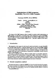
Figure 3. Intermediate state of preflow-push algorithm. Each node is labeled with its height h and its excess inflow e. Each edge is labeled with its maximum capacity and current flow. Dashed edges are edges in the residual graph.

2.

Amorphous data-parallelism and the Galois system

In this section, we describe the concept of amorphous dataparallelism and argue that optimistic parallel execution is essential to exploit this parallelism in general. We also describe the Galois system, which is a baseline system that uses optimistic parallel execution to exploit amorphous data-parallelism. 2.1

Example: Preflow-push

To introduce the concept of amorphous data-parallelism, we use the preflow-push algorithm for computing maxflows in directed graphs [5]. The pseudocode is shown in Figure 2, and the directed graph in Figure 3 shows an intermediate state of a preflow-push computation on a simple graph. Unlike in maxflow algorithms based on augmenting paths, nodes in this algorithm can temporarily have more flow coming into them than going out. In Figure 3, the excess inflow at a node n (other than the source and sink) is denoted by the label e(n) on that node. Each node also has a label called height, shown as h(n), which is an estimate of the distance from that node to the sink in the residual graph. Nodes with nonzero excess inflow are called active nodes; in Figure 3, nodes a and b are active nodes. The algorithm repeatedly selects an active node node and performs two operations called push and relabel. The push operation tries to increase the flow along some outgoing edge (node→neighbor) to eliminate the excess flow at node if possible; if it succeeds, the flow on that edge is updated. Increasing the flow to neighbor may cause neighbor to become active; if node still has excess in-flow, it remains an active node. To ensure that flow moves from the source to the sink, the push operation can only push flow downhill (that is, from a node to a lower-height neighbor). Height estimates can be adjusted by relabel operations.

The push and relabel computation at an active node is called an activity. Since active nodes can be processed in any order, there is a natural parallelism that arises from processing multiple active nodes concurrently, provided their neighborhoods are disjoint. This parallelism differs from regular data-parallelism in the following crucial ways. • Conventional data-parallelism arises in algorithms that operate

on dense matrices and vectors. The preflow-push algorithm performs operations over a graph data structure. An irregular, pointer-based structure like a graph is far more difficult to reason about than matrices and vectors. • In preflow-push, nodes become active nodes dynamically, based

on runtime data values. In regular algorithms, however, parallelism is independent of runtime values. • Identifying active nodes that can be processed concurrently

requires knowledge of the structure of the graph, which is known only at runtime. 2.2

Amorphous Data-parallelism

The parallelism in the preflow-push algorithm is an instance of a more general pattern of parallelism called amorphous dataparallelism that arises in irregular algorithms that operate on pointer-based data structures like graphs. At each point during the execution of such an algorithm, there are certain nodes or edges in the graph where computation might be performed. Performing a computation may require reading or writing other nodes and edges in the graph. The node or edge on which a computation is centered is called an active element, and the computation itself is called an activity. It is convenient to think of an activity as resulting from the application of an operator to the active node. We refer to the set of nodes and edges that are read or written in performing the activity as the neighborhood of that activity. In Figure 1, the filled nodes represent active nodes, and shaded regions represent the neighborhoods of those active nodes. Note that in general, the neighborhood of an active node is distinct from the set of its neighbors in the graph. In some algorithms like Delaunay mesh refinement, activities may modify the graph structure of the neighborhood by adding or removing graph elements. In general, there are many active nodes in a graph, so a sequential implementation must pick one of them and perform the appropriate computation. In some algorithms such as preflow-push, the implementation is allowed to pick any active node for execution. We call these algorithms unordered algorithms. In contrast, other algorithms dictate an order in which active nodes must be processed. Event-driven simulation is an example: the sequential algorithm for event-driven simulation processes messages in global time-order. We call these ordered algorithms. A natural way to program these algorithms is to use the Galois programming model [12], which is a sequential, object-oriented programming model (such as sequential Java) augmented with two Galois set iterators: • Unordered-set iterator: foreach (e : Set S) do B(e) The loop

body B(e) is executed for each element e of set S. The order in which iterations execute is indeterminate and can be chosen by the implementation. There may be dependences between the iterations. When an iteration executes, it may add elements to S. • Ordered-set iterator: foreach (e : OrderedSet S) do B(e)

This construct iterates over an ordered set S. It is similar to the unordered set iterator above, except that a sequential implementation must choose a minimal element from set S at every

iteration. When an iteration executes, it may add new elements to S. Note that these iterators have a well-defined sequential semantics. The pseudo-code in Figure 2 uses the unordered Galois set iterator. The unordered-set iterator expresses the fact that active nodes can be processed in any order. Figure 1 shows how opportunities for exploiting parallelism arise in graph algorithms: if there are many active elements at some point in the computation, each one is a site where a processor can perform computation, subject to neighborhood and ordering constraints. When active nodes are unordered, the neighborhood constraints must ensure that the output produced by executing the activities in parallel is the same as the output produced by executing the activities one at a time in some order. For ordered active elements, this order must be the same as the ordering on set elements. Definition 2.1. Given a set of active nodes and an ordering on active nodes, amorphous data-parallelism is the parallelism that arises from simultaneously processing active nodes, subject to neighborhood and ordering constraints. Amorphous data-parallelism is a generalization of conventional data-parallelism in which (i) concurrent operations may conflict with each other, (ii) activities can be created dynamically, and (iii) activities may modify the underlying data structure. 2.3

Baseline implementation: optimistic parallel execution

In the baseline programming model, the application programmer writes sequential code in a conventional object-oriented language, augmented with Galois set iterators. Concurrent data structures are implemented in a data structure library, similar to the Java collections library, that contains implementations of common data structures such as graphs and trees. In the baseline execution model, the graph is stored in sharedmemory, and active nodes are processed by some number of threads. A free thread picks an arbitrary active node and speculatively applies the operator to that node, making calls to the graph class API to perform operations on the graph as needed. The neighborhood of an activity can be visualized as a blue ink-blot that begins at the active node and spreads incrementally whenever a graph API call is made that touches new nodes or edges in the graph. To ensure that neighborhood constraints are respected, each graph element has an associated logical lock that must be acquired by a thread before it can access that element. Locks are held until the activity terminates. Lock manipulation is performed by the code in the graph API call, not in the application code. If a lock cannot be acquired because it is already owned by another thread, a conflict is reported to the runtime system, which rolls back one of the conflicting activities. To enable rollback, each graph API method that modifies the graph makes a copy of the data before modification. Like lock manipulation, rollbacks are a service implemented by the library and runtime system. Logical locks provide a simple approach to ensuring that neighborhood constraints are respected, but they can be restrictive since they require neighborhoods of concurrent activities to be disjoint (such as activities i3 and i4 in Figure 1). Non-disjoint neighborhoods are permissible if the activities do not modify nodes and edges in the intersection for example. One solution is to use commutativity conditions [12] that describe more complicated conditions under which two activities can be processed in parallel; to keep the discussion simple, we do not describe this here. If active elements are not ordered, the activity terminates when the application of the operator is complete and all acquired locks are released. If active elements are ordered, active nodes can be processed in any order, but they must commit in serial order. This can be implemented using a data structure similar to a reorder buffer in

out-of-order processors [12]. In this case, locks are released when the activity commits. Since amorphous data-parallelism in irregular algorithms is a function of runtime values, it is not possible to come up with closed-form estimates of the amount of parallelism in these algorithms in general. One measure of amorphous data-parallelism is the number of active nodes that can be processed in parallel at each step of the algorithm for a given input, assuming that (i) there is an unbounded number of processors, (ii) an activity takes one time step to execute, (iii) the system has perfect knowledge of neighborhood and ordering constraints so it only executes activities that can complete successfully, and (iv) a maximal set of activities, subject to neighborhood and ordering constraints, is executed at each step. This is called the available parallelism at each step, and a function plot showing the available parallelism at each step of execution of an irregular algorithm for a given input is called a parallelism profile. In this paper, we will present parallelism profiles produced by ParaMeter, a tool implemented on top of the Galois system [14]. 2.4

The Galois system

In this section, we describe how the Galois system [12] implements the baseline model presented in the previous section. The goal is to give the reader the right context for understanding how the optimizations described in Section 3 can be implemented. The system has the following components: a library of data structures commonly used in irregular applications, a set of conflict manager objects (CMs) that implement neighborhood constraints, a Galois compiler that transforms programs to enable safe parallel execution, and a runtime system that orchestrates the parallel execution. Library of data structures The system provides a library of parallel implementations of data structures, such as graphs, maps, and sets, which are commonly used in irregular algorithms. Since a general implementation may introduce unnecessary overhead because it provides functionality that is not required for a particular application, the library provides several customized versions for each type. For example, some applications may require a directed graph, while others require an undirected graph. Some applications may require the ability to attach data to graph edges (e.g., to track edge capacities in preflow-push). Programmers can either use one of the existing implementations or provide new ones. For a data structure implementation to be suitable for the Galois system it must satisfy two properties: (i) it should implement an existing abstract data type, and (ii) operations on the data structure must appear to execute atomically. Conflict managers Each shared object accessed inside a foreach section must be associated with a special conflict manager object (CM) that is responsible for enforcing neighborhood constraints. For example, a conflict manager for a graph class must ensure that two activities do not attempt to modify the same graph node. The system provides conflict managers for all library types. These conflict managers implement neighborhood constraints either by logical locking or commutativity conditions [12]. CMs intercept method invocations on data structures and acquire logical locks, or they evaluate commutativity conditions to ensure that multiple activities are independent. For example, a CM for a graph will intercept a call to getNeighbors(n) and acquire logical locks on node n and its neighbors. A baseline conflict manager can be used in cases where higherlevel semantics cannot be easily exploited. The baseline CM essentially acts as an exclusive lock on the entire object; invoking any method on the data structure will attempt to acquire this lock. The baseline CM provides a conflict detection policy similar to that of object-based software transactional memories.

@Wrap ( c o n f l i c t M a n a g e r = G r a p h C o n f l i c t M a n a g e r ) c l a s s Graph { p u b l i c S e t g e t N e i g h b o r s ( Node n ) { return n . neighbors ; } / / r e s t o f methods }

Figure 4. Source code of the graph class. Since multiple concurrently executing activities can interact with the conflict manager, the CM’s operations should be atomic. Conflict managers are designed to operate with particular abstract data types, not particular concrete implementations of data structures. Thus, a CM for an abstract data type can protect any data structure implementing that type. The Galois compiler An irregular algorithm written in the Galois system is a standard Java program augmented with Galois set iterators. The Galois compiler transforms Galois programs with set iterators into a standard Java program that executes on top of the Galois runtime system. First, a preprocessing pass transforms foreach statements to calls to the Galois runtime system. This transformation is implemented using the Polyglot source-to-source transformation toolkit [20]. The transformed program is now a valid, parallel Java program and can run on any Java virtual machine, but it cannot be executed safely in parallel, as the data structures accessed from within the set iterators do not enforce neighborhood constraints. To produce a program that can safely execute in parallel, a second pass wraps each shared data structure. This transformation is implemented in the Soot compiler framework [26]. First, each data structure is associated with an appropriate conflict manager, as specified by a Java annotation. For every method belonging to a data structure manipulated by the client code, the compiler introduces a call to a conflict manager method, called the prolog, at the entry point of the method. Similarly, at each exit point (i.e., before returning a value or throwing an exception), it introduces a call to an epilog method. The purpose of prolog and epilog is to determine if neighborhood constraints are violated. These methods also record undo actions, which allow the effects of an iteration to be undone if the iteration must be rolled back. As an example, consider Figure 4, which shows an implementation of the getNeighbors method of the Graph class. The code includes a directive to the compiler, @Wrap, that specifies which specific conflict manager needs to be instantiated. Based on this information, the compiler adds a field of the indicated type within the Graph class and then inserts invocations of prologs and epilogs appropriately, as shown in Figure 5. Each invocation passes a unique method identifier, the actual parameters, and the return value (in the case of epilogs). One possible implementation of conflict detection for the getNeighbors method would be as follows. In the prolog, the conflict manager acquires a lock on the argument node. This prevents any other iteration from reading or writing that node. In the epilog, the neighbors are known, and the conflict manager acquires locks on those nodes as well. Because this method does not modify the graph, no undo action is recorded by the conflict manager. Note that the wrapped code includes checks to test whether conflict management is required; conflict management need not be performed during sequential execution or after applying certain optimizations, as we describe in Section 3. The Galois runtime system The Galois runtime system coordinates the parallel execution of the application. For every foreach construct, a number of parallel iterations are launched to implement the Galois set iterators. Each iteration works on an active node from the workset and executes speculatively. Before operating on a piece of shared data, an iteration interacts with the appropriate conflict manager to ensure that the object is accessed safely. In the case

c l a s s Graph { G r a p h C o n f l i c t M a n a g e r cm ; / / added by t h e w r a p p e r p u b l i c S e t g e t N e i g h b o r s ( Node n ) { b o o l e a n cmOn = Runtime . isCmOn ( ) ; i f ( cmOn ) cm . p r o l o g ( ’ g e t N e i g h b o r s ’ , t h i s , n ) ; S e t r e s u l t = n . n e i g h b o r s ; i f ( cmOn ) cm . e p i l o g ( ’ g e t N e i g h b o r s ’ , t h i s , n , r e s u l t ) ; return r e s u l t ; } / / r e s t o f methods }

Figure 5. Instrumented code of the graph class. of a conflict, an arbitration mechanism aborts one of the conflicting iterations and rolls back the speculative changes. Each iteration has an associated undo log, where the conflict manager stores the appropriate undo information. If an iteration successfully finishes its execution, the runtime clears all logs associated with the iteration and releases the abstract locks the iteration acquired during its execution.

3.

Optimizations

As described in Section 2, optimistic parallel execution is very general and can exploit parallelism in a wide variety of algorithms. However, because of its generality, it implements functionality that may not be needed for a particular irregular algorithm, leading to unnecessary overheads. Optimizing compilers provide a useful analogy for understanding how to structure a system for optimistic parallel execution of programs. To implement a powerful mechanism like procedure invocation, most compilers will generate relatively heavy-weight code by default, but will generate light-weight customized code for special cases of that construct that arise frequently in practice, such as tail-recursive calls. By analogy, a system for optimistic parallel execution should provide a collection of services that are adequate to exploit amorphous data-parallelism in any program, but it should also be possible to exploit structure in a particular irregular algorithm to “turn off” some of these services and provide lighter-weight parallelization if these services are not required to exploit parallelism. One difficulty with this agenda is that, in spite of a lot of effort by the community [17, 22, 25], we do not yet have a systematic way of talking about structure in algorithms in the context of parallelism. Fortunately, the framework of amorphous data-parallelism provides an approach to discussing algorithmic structure relevant to our optimizations. The major sources of runtime overheads in the baseline system described in Section 2 are the following. • Dynamic assignment of work: Threads go to the centralized

workset to get work. This requires synchronization; moreover, if there are many threads and the computation performed in each activity is small, contention between threads will limit speedup. • Enforcing neighborhood constraints: Acquiring and releasing abstract locks on neighborhood elements can be a major source of overhead. • Copying data for rollbacks: When an activity modifies a graph element, a copy of that element is made to enable rollbacks. • Aborted activities: When an activity is aborted, the computational work performed up to that point by that activity is wasted. Furthermore, the runtime system needs to take corrective action to roll back the activity, which adds to the overhead. In this section, we describe three optimizations for reducing these overheads. Section 3.1 introduces the notion of cautious im-

plementations of operators and argues that under some fairly general conditions, optimistic parallel execution can be implemented without making back-up copies of data for rollbacks. This optimization is important because in practice, most irregular algorithms have cautious operator implementations. Section 3.2 describes a one-shot implementation of operators, which targets the overheads from aborted activities. Intuitively, one-shot execution detects conflicts as early as possible to avoid wasting effort in performing computations that ultimately get aborted. Section 3.3 describes iteration coalescing, which can be viewed as a data-centric version of loop chunking [23]. It targets the overheads of dynamic work assignment and the cost of acquiring and releasing abstract locks. In some programs, it can also improve the exploitation of locality of reference. 3.1

Cautious implementations of operators

As mentioned in the introduction, Blandford et al.’s implementation of Delaunay mesh refinement [1] uses an optimistic parallel execution strategy similar to the one used in the Galois system, but it rolls back conflicting computations without using logs or backup copies of modified data. However, logs or backup copies of modified data are needed for other algorithms such as event-driven simulation. In this section, we describe the program structure that permits optimistic parallel execution to be performed without making backup copies of modified data, and how this optimization can be implemented in the Galois system. Definition 3.1. An implementation of an operator is said to be cautious if it reads all the elements of its neighborhood before it modifies any of them. Operators can usually be implemented in different ways: for example, one implementation might read node A, write to node A, read node B, and write to node B, in that order, whereas a different implementation might perform the two reads before the writes. By Definition 3.1, the second implementation is cautious, but the first one is not. If (i) the implementation of an operator is cautious and (ii) active nodes are unordered, all conflicts are detected before any modifications are made to the graph. Logical locks associated with graph elements are acquired during the read-only phase of the operator. If a lock cannot be acquired, there is a conflict, and the computation is rolled back simply by releasing all locks acquired up to that point; otherwise, all locks are released when the computation finishes. The runtime system ensures that once the “fail-safe point” is passed, the computation is not rolled back. This is possible in general only for unordered algorithms; for ordered algorithms, a conflicting activity a1 with higher priority may require an activity a2 to be rolled back after a2 has begun to make modifications to the graph. Notice that exploiting cautious implementations also reduces the cost of acquiring abstract locks, because after the failsafe point has been passed, graph API calls do not need to check whether locks have been acquired on graph elements. We refer to this as a zero-copy implementation. In our experience, the straight-forward implementations of most operators are cautious. For example, the operator in Delaunay mesh refinement is cautious because the cavity of a bad triangle must be determined before it can be retriangulated. Other examples are Boruvka’s algorithm for computing minimal spanning trees (MST) and the preflow-push algorithm for maxflow computations. In contrast, the operator for the well-known Delaunay triangulation algorithm of Guibas, Knuth and Sharir [9, 13] does not have a naturally cautious implementation. The operator in this algorithm inserts a point into a triangle, splitting that triangle into three smaller triangles. The Delaunay condition may be violated for the new triangles as well as for triangles in the vicinity of the original triangle, so the

1 wl . add ( g r a p h . g e t S o u r c e ( ) ) ; 2 f o r e a c h ( Node node : wl ){ 3 N e i g h b o r h o o d . add ( node ) ; 4 N e i g h b o r h o o d . add ( g . g e t N e i g h b o r s ( node ) ) ; 5 ONE SHOT . s e t ( N e i g h b o r h o o d ) ; 6 g . r e l a b e l ( node ) ; 7 f o r ( Node n e i g h b o r : g . g e t N e i g h b o r s ( node ) ) { 8 / / r e s t o f t h e c o d e r e m a i n s t h e same 9 } 10 }

Figure 6. Preflow-push code with the one-shot optimization.

algorithm performs a series of graph mutations called edge flips to restore the Delaunay condition for all triangles. The only way to determine which edges need to be flipped is to perform edge flipping incrementally, so the natural implementation of this operator is not cautious. Notice that, in principle, every operator has a trivial cautious implementation that acquires locks on all graph elements before beginning the computation. The obvious disadvantage of this implementation is that it prevents the exploitation of parallelism. However, for some operators that do not have a natural cautious implementation, it may be possible to judiciously over-approximate the neighborhood to obtain a cautious implementation without hurting parallelism too much. There is a tradeoff in these cases between the exploitation of parallelism and the complexity of operator implementation. We leave the exploration of this tradeoff for future research. Implementation in Galois: The cautious optimization requires the user to indicate whether the operator implementation is cautious. In principle, compiler analysis can be used in many cases to determine whether an operator implementation is cautious, but we have not yet incorporated this analysis into our compiler. Each conflict manager type provides a cautious mode of operation, in which the conflict manager object does not store undo information when intercepting methods. Additionally, after intercepting the first method that modifies the data structure, it turns off all conflict management for the current iteration. The user can direct the compiler to instrument the application either in cautious or standard mode. Related work: To the best of our knowledge, we are the first to identify cautiousness as a general property of many irregular algorithms. However, cautiousness has been used implicitly in handwritten parallel implementations of some irregular applications. The DMR implementation of Blandford et al. uses “test” locks; if locks cannot be acquired, the operation attempting to acquire the lock is aborted and retried at another time. Therefore, this DMR code first attempts to grab all of its locks and only begins performing updates to the cavity after these locks have been successfully acquired. We get the benefit of this optimization by exploiting the general property of cautiousness in the implementations of operators. Recently, Lubllinerman et al. have proposed a parallel programming and implementation model for unordered algorithms with cautious operator implementations [16]. Zero-copy implementation should not be confused with two-phase locking in databases, since under two-phase locking, updates to locked objects can be interleaved arbitrarily with acquiring locks on new objects. 3.2

One-shot implementation

In some algorithms, it is possible to predict the neighborhood of an activity without performing any computation. In other algorithms, it is possible to compute fairly tight over-approximations to neighborhoods. For example, in the preflow-push algorithm, the neighborhood of an active node consists of its neighbors in the graph

and the edges between the active node and those neighbors. In such cases, it is possible to acquire all locks needed by an activity before any computation is performed. If no conflict is detected, locking can be disabled for the rest of the activity. This is called the oneshot optimization. The advantages of this optimization are similar to those obtained by exploiting cautious operators, but the overhead of aborts is even lower since no computation is performed before conflicts are detected. In principle, the one-shot technique can be used for any algorithm since one approximation to the neighborhood of an activity is the entire graph. However, as in the case of cautious operators, over-approximating neighborhoods may reduce parallelism and increase the number of aborted activities. Implementation in Galois: We require users to specify whether the implementation of the operator is one-shot. However, the implementation in the Galois system also requires that the user provide code to identify an operator’s neighborhood. The Galois system includes a singleton object, called ONE SHOT, which provides the method ONE SHOT.set(Collection). The user identifies a set of objects that constitute the neighborhood of an active element and invokes ONE SHOT.set() on that collection. The Galois system then acquires the appropriate locks and turns off conflict detection for the remainder of the iteration. As in the case of the cautious optimization, the system does not record undo actions. Figure 6 shows how the preflow-push code has been modified so that the one-shot optimization is enabled. The only changes from Figure 2 are the addition of lines 3, 4, and 5. Related work: One-shot optimization is analogous to pessimistic locking techniques developed for transactions [3, 18]. In the same spirit as one-shot execution, pessimistic approaches eliminate the need for expensive conflict detection during parallel execution. Static analysis is used to determine which locks must be acquired. Since static analysis techniques for programs that manipulate pointers are not very accurate, pessimistic locking implementations may end up locking the entire graph. Notice that in our approach, application programs do not manipulate pointers directly; instead, they make calls to a graph API that is implemented by the library. Static analysis of this higher-level code can exploit the semantics of API calls, so in principle, it can produce more accurate results than static analysis of low-level C code that manipulates pointers directly. We have not finished the implementation of this analysis in our system, so we currently rely on user directives. 3.3

Iteration coalescing

The final optimization we discuss is iteration coalescing, which can be viewed as a data-centric version of loop chunking [23]. In the context of regular programs, researchers have long recognized that dynamically assigning work to threads has significant overhead, so OpenMP [21], for example, supports chunking of iterations, which permits multiple iterations to be handed out to a thread at a time. In the Galois baseline implementation, each iteration executes a single activity. This means that the processing of an active element incurs two overheads: (i) acquiring work from the workset, and (ii) acquiring abstract locks for the neighborhood. Iteration coalescing reduces these overheads by breaking the one-to-one correspondence between iterations and activities. In an OpenMP-like implementation, a single iteration would grab multiple active elements from the workset, reducing the cost of accessing the workset. However, the neighborhoods for these activities may not have much overlap, so the cost of locking may not necessarily be reduced with this strategy. A smarter, data-centric approach would chunk activities whose neighborhoods overlap. One way to achieve this is the following: in algorithms in which active elements are generated dynamically

(e.g., preflow-push, where an activity might push flow to a node, which then becomes active), an iteration that generates a new active element processes that element without putting it on the workset. This is effective because in many algorithms, including preflowpush and Delaunay mesh refinement, the neighborhood of the new activity is likely to overlap with the neighborhood of its parent activity. This allows us to exploit a phenomenon called lock locality: because the neighborhoods of chunked activities overlap, the number of new locks that need to be acquired for the second activity is reduced. The better the lock locality of a program, the more we can amortize the cost of acquiring locks. Notice that a data-centric work assignment strategy also increases data locality, improving cache performance. There are algorithms that may not benefit from this strategy; for example, in ray-tracing, the neighborhoods of child rays may not overlap much with the neighborhood of their parent ray. The downside of iteration coalescing is that it increases the effective neighborhood size of the active elements processed by an iteration, which increases the likelihood of conflicts. We mitigate this effect in two ways. If a conflict is detected, only the currently executing activity is rolled back; previously executed activities can be safely committed. Second, we place an upper bound on how many iterations can be coalesced, using application-specific heuristics. Iteration coalescing is applicable only to unordered algorithms, and the implementation described above is most effective for algorithms that have the following characteristics: (i) the amount of computation in each activity is relatively small compared to the overheads of accessing the workset and acquiring locks, (ii) active elements are generated dynamically, and (iii) the neighborhood of a dynamically created activity overlaps significantly with the neighborhood of its parent activity. Implementation in Galois: The implementation of iteration coalescing is the following. Each iteration maintains an iteration-local workset. When an activity generates new active elements, these active elements are placed on the local workset. When an activity is completed, the iteration gets work from its local workset if possible, without releasing abstract locks. This process continues until either (i) the maximum coalescing factor is reached, (ii) a conflict is detected, or (iii) the local workset is empty. When the iteration finishes, it releases all its abstract locks. If a conflict is detected, the currently executing activity is rolled back, and work executed earlier is committed. Any work left on the local workset is moved to the global workset. Related work: We do not know of any analog of data-centric chunking in the literature. However, the implementation of partial rollback of iterations during conflict handling is similar to the implementation of partial rollback of nested transactions [19, 24]. In that setting, when a nested transaction encounters a conflict, it is possible to only roll back the nested transaction, rather than the parent transaction as well. In a similar vein, when we encounter a conflict while performing iteration coalescing, we need only abort the currently executing activity, rather than all previously completed activities.

4.

Experimental evaluation

In this section, we report our evaluation of the three optimizations described in Section 3. We used two machines for our experiments. One machine was a Sun Fire X2270 (Nehalem server) running Ubuntu Linux version 8.06. The system contains two quad-core 2.93 GHz Intel Xeon processors. The 8 CPUs share 24 GB of main memory. Each core has two 32 KB L1 caches and a unified 256 KB L2 cache. Each processor has an 8 MB L3 cache that is shared among the cores. We

Program DMR Boruvka Preflow-push SP

Time/iteration (µsec.) 100 3 0.64 0.13

Table 1. Average serial runtime per iteration.

used the Sun HotSpot 64-bit server virtual machine version 1.6.0. The second platform was a Sun UltraSPARC T2 (Niagara 2 server) running Solaris 10. The system consists of a single chip with 8 cores running at 1.4 GHz. Each core is 8-way hyperthreaded for a total of 64 virtual cores. Each core has an 8 KB L1 data cache and a 16 KB L1 instruction cache. The 8 cores share an 8-bank, uniform access, 4 MB L2 cache. We used the following benchmark programs. The Lonestar 2.0 benchmark suite is a collection of five irregular applications: Delaunay triangulation, Delaunay mesh refinement (DMR), survey propagation (SP), Barnes-Hut, and agglomerative clustering. The operators for Delaunay triangulation and agglomerative clustering are not cautious, so the optimizations discussed in this paper are not useful for these codes (although agglomerative clustering might benefit from iteration coalescing). The most time-consuming part of the Barnes-Hut code iterates over a read-only tree, and it can be parallelized trivially. Therefore, we focused on DMR and SP from the Lonestar benchmark suite. In addition, we evaluated the optimizations on an implementation of Boruvka’s algorithm for building minimal spanning trees [6] and an implementation of the preflow-push algorithm for computing maximal flows in a directed graph [8]. These two benchmarks will appear in the next release of the Lonestar suite. The benchmarks and the Galois runtime system are written in Java. To account for the effects of JIT compilation, each benchmark was run nine times, and the median runtime is reported. We also minimize the influence of garbage collection by maximizing the size of the heap used by the JVM. Table 1 shows the average time per activity (iteration) when sequential Java implementations of these algorithms are executed on one core of the Nehalem server. These times span a wide range, allowing us to evaluate the effectiveness of the optimizations on programs with very different behavior. To measure the performance improvement from the optimizations introduced in this paper, we used baseline Galois versions of the four benchmarks. For DMR, preflow-push, and SP, the baseline implementation uses Metis [11] to partition the input graph so that there are 4 partitions per thread in each of the experiments described below. Each partition has a lock that must be acquired by a thread that wants to access a node or edge in that partition. The over-decomposition permits a thread to do useful work even if one of its partitions is temporarily locked by a different thread [15]. It is difficult to partition the underlying graph in the Boruvka MST algorithm since it is ultimately coalesced into a single node, so we do not use partitioning for this algorithm; instead we associate locks with nodes and edges of the graph. We do not include the time for graph partitioning in the runtimes reported below. Figure 7 shows runtimes for Delaunay mesh refinement, Boruvka’s algorithm, preflow-push, and survey propagation. For Delaunay mesh refinement, Boruvka’s algorithm, and preflowpush, we report the runtime of a baseline version (i.e., with no optimizations), versions with a single optimization applied, and a version with all the applicable optimizations enabled. For reasons described in Section 4.4, we report the normalized runtime per 10 million activities and do not evaluate the baseline version for survey propagation. Figures 8 and 9 show detailed experimental results. Among

1 W o r k s e t ws = new W o r k s e t ( g . b a d T r i a n g l e s ( ) ) ; 2 f o r e a c h ( T r i a n g l e node : ws ) { 3 i f ( node no l o n g e r i n g r a p h ) 4 continue ; 5 C a v i t y c = new C a v i t y ( node ) ; 6 c . expand ( ) ; 7 c. retriangulate (); 8 g . removeNodes ( c . g e t O l d N o d e s ( ) ) ; 9 g . addNodes ( c . getNewNodes ( ) ) ; 10 g . a d d E d g e s ( c . getNewEdges ( ) ) ; 11 ws . add ( c . b a d T r i a n g l e s ( ) ) ; 12 }

1 2 3 4 5 6 7 8 9 10 11

Graph g = / ∗ i n p u t g r a p h ∗ / MST mst = new MST( g ) ; / / i n i t i a l i z e MST f r o m g W o r k s e t ws = new W o r k s e t ( g . g e t N o d e s ( ) ) ; f o r e a c h ( Node n : ws ) { Edge e = minWeight ( g . g e t N e i g h b o r s ( n ) ) ; Node l = c o n t r a c t ( e ) ; / / c o n t r a c t e d g e e , f o r m i n g l / / Add e d g e e t o t h e MST mst . addEdge ( e ) ; / / add new node b a c k t o w o r k s e t ws . add ( l ) ; }

Figure 12. Pseudocode for Boruvka’s algorithm.

Available Parallelism 5000 10000

Available Parallelism 4000 8000 12000

Figure 10. Pseudocode for Delaunay mesh refinement.

196

0

0

57

0 0

10

20 30 40 Computation Step

50

50

100 Computation Step

150

200

Figure 13. Parallelism profile for Boruvka’s algorithm.

Figure 11. Parallelism profile for Delaunay mesh refinement. 4.1.1 other numbers, these figures show (i) the abort ratio (the number of aborted iterations divided by the number of aborted and committed iterations)1 , (ii) the average and maximum number of locks acquired by an activity, (iii) change (percent improvement of the running time of an optimized version over the baseline version, for the same number of threads). 4.1 Delaunay mesh refinement DMR is an irregular algorithm that uses iterative refinement to eliminate badly shaped triangles from a mesh of triangles while ensuring that all triangles satisfy a certain geometric property called the Delaunay condition. To fix a bad triangle, a new point is added at its circumcenter, and the bad triangle and some of its neighbors are replaced with new triangles; these neighboring triangles are said to lie in the cavity of the bad triangle. Re-triangulating a cavity may generate new bad triangles but it can be shown that at least in 2D, this iterative refinement process will ultimately terminate and produce a mesh without bad triangles. Figure 10 shows the pseudocode. Each iteration of the while loop refines one bad triangle. Each bad triangle is an active node, and the cavity generated while processing a bad triangle is the neighborhood of the active node. The operator implementation in DMR is cautious because it expands a cavity (line 6) before modifying anything in its neighborhood (lines 8–10). However, the one-shot optimization cannot be used because the cavity is a function of the shape and distribution of the triangles in the mesh. Therefore, absent any knowledge of geometry [4], we cannot place a bound on a cavity (i.e., neighborhood of an active node) before executing an iteration. 1 It

is important to remember that the cost of aborted iterations depends both on the abort ratio and on how much work aborted iterations perform on average before being rolled back. A high abort ratio is not necessarily fatal to performance if most aborted iterations are rolled back before they perform much work, as is often the case when some of the optimizations described in this paper are applied.

Results

The input mesh consists of 550,000 randomly generated triangles, of which approximately half are “bad.” Figure 11 shows the parallelism profile for this application. The parallelism increases initially because conflicts between bad triangles are reduced as the mesh is refined and becomes larger. As bad triangles get eliminated from the mesh, the amount of parallelism drops. The cautious implementation of the operator gives a small but measurable improvement of 12–15%. Figure 8 shows that the average number of locks held by an iteration in both the baseline and cautious implementations is close to 1. This means that most cavities lie within a single partition, showing the effectiveness of the partitioner for this problem. In the worst case, a cavity touches 3–4 partitions even when the number of partitions is 64 (for 16 threads). Iteration coalescing provides modest improvements of 6–9% for this code. Each iteration of DMR performs a lot of computation, so the relative cost of getting work from the workset and of acquiring locks is small, limiting the benefits of iteration coalescing. Furthermore, iteration coalescing causes the abort ratio to increase, as can be seen in Figure 8, since the effective neighborhood of an iteration increases. On both machines, the best version uses only the cautious operator implementation. Speedup over serial code is 6.86 on the Nehalem server and 8.5 on the Niagara 2 server, obtained on 8 cores/16 threads in both cases. 4.2

Boruvka’s algorithm

Boruvka’s algorithm is a method for finding the minimum spanning tree (MST) of a graph (Figure 12). The intuition behind this algorithm is that the MST starts as a forest, with each node in its own component. Each component then finds the lightest weight edge that connects it to another component, adds that edge to the MST and merges the two components together. The membership of nodes in components can be maintained by contracting the nodes along the lightest edge into a single component with the same connectivity as the two original components. The original components are removed from the graph. A union-find data structure may also

●

●

●

●

●

● ●

●

● ●

4 8 Threads

16

1

(1) Delaunay mesh refinement

2

4 8 Threads

16

0

0

0 2

●

●

0 1

10000

2000

● ●

10000 20000

4000

25000

Execution Time (ms) 10000 25000

●

1

(2) Boruvka’s algorithm

2

4 8 Threads

16

1

(3) Preflow-push

2

4 8 Threads

16

(4) Survey propagation

●

2

4 8 Threads

16

(1) Delaunay mesh refinement

● ●

250000 ●

●

●

●

1

2

4 8 Threads

16

(2) Boruvka’s algorithm

0

0

●

●

0

●

0 10000

●

●

100000

●

●

1

250000

●

100000

30000

Execution Time (ms) 100000 250000

(a) Execution times on Nehalem

1

2

4 8 Threads

16

(3) Preflow-push

1

2

4 8 Threads

16

(4) Survey propagation

(b) Execution times on Niagara 2 ●

Baseline Coalescing

Cautious One−shot

Coalescing+Cautious Coalescing+One−shot

Figure 7. Execution times on Nehalem (top) and Niagara 2 (bottom). Dotted lines show serial execution time.

be used to maintain the components but we do not evaluate such a variant in this paper. The active nodes are the nodes of the graph. To update the connectivity in the contracted component, the neighbors of the node incident on the lightest edge must be updated as well. The neighborhood of an active node therefore consists of the set of neighbors of the active node and the neighbors of the node incident on the lightest edge. It is difficult to use partitioning with this algorithm since it contracts the graph repeatedly until only one node is left. Therefore, we associate locks with nodes and edges in this code. The operator implementation given in Figure 12 is cautious. Strictly speaking, the one-shot implementation cannot be used because, without executing the code, we do not know which edge incident on the active node is the lightest one. However, it is possible to over-approximate the neighborhood as the set of neighbors of the active node together with the set of neighbors of these nodes. This over-approximation permits us to evaluate the one-shot optimization. 4.2.1

Results

The input to the algorithm is a 2D mesh with 202,500 nodes. Figure 13 shows the parallelism profile for this application. Initially, there is a high amount of parallelism, but it quickly tapers off as the graph becomes smaller. Figure 8 shows that the cautious implementation optimization produces an improvement of about 9–22% over the baseline implementation on the Nehalem server, and 20–23% on the Niagara 2 server. The operator in Boruvka’s algorithm has two phases: the

first phase finds an edge to contract, and the second phase performs edge contraction. The first phase only reads the graph, so cautiousness only helps during the edge-contraction phase, where nodes can be removed and edges re-targeted without acquiring locks or recording undo actions. The one-shot optimization degrades performance substantially on the Nehalem server, and improves performance by 4–9% on the Niagara 2 server. Applying this optimization requires overapproximating the neighborhood, as explained above, which increases locking overheads as well as the probability of conflicts. Figure 8 shows that the average number of locks held by an activity is roughly twice the number held in the baseline (or cautious) implementation. Furthermore, the operator also performs more computation in traversing the graph. In this code, the useful work per iteration is an order of magnitude lower than in DMR. Therefore, we would expect iteration coalescing to be more useful than in the case of DMR. Iteration coalescing results in an improvement of 1–8% over the baseline in the two machines. To explain these results, we appeal to lock locality. We can estimate the lock locality in the algorithm by examining the average number of locks acquired per activity, as seen in Figure 8. When applying iteration coalescing to a program with high lock locality, we expect to acquire fewer locks per activity, as many necessary locks will have been acquired by earlier activities. We see that this is not the case in Boruvka’s algorithm; the average number of locks acquired per activity does not change when we apply iteration coalescing. Thus, the primary benefit of coalescing is to reduce workset overheads. However, combining iteration coalescing with

Delaunay m esh refinem ent abort ratio Serial

ave lock

m ax lock

Boruvka's algorithm Nehalem tim e change (m s) 21025

Baseline 1 0.00 2 0.01 4 0.01 8 0.00 16 0.01 Cautious 1 0.00 2 0.02 4 0.01 8 0.00 16 0.01 One-shot

Niagara 2 tim e change (m s)

abort ratio

ave lock

m ax lock

142050

Nehalem tim e change (m s) 1243

Niagara 2 tim e change (m s) 5665

1.02 1.04 1.04 1.06 1.07

3 30514 3 16066 3 8522 4 5153 3 3499

0.00% 0.00% 0.00% 0.00% 0.00%

240038 121845 64449 33868 20386

0.00% 0.00% 0.00% 0.00% 0.00%

0.00 0.00 0.00 0.01 0.03

5.67 5.66 5.67 5.67 5.67

39 34 45 42 34

4390 2755 1569 1083 1428

0.00% 0.00% 0.00% 0.00% 0.00%

32920 16748 8599 4564 2649

0.00% 0.00% 0.00% 0.00% 0.00%

1.02 1.02 1.04 1.05 1.07

3 26999 3 13974 3 7260 4 4679 4 3067

11.52% 13.02% 14.81% 9.20% 12.35%

203080 104739 54346 29070 16768

15.40% 14.04% 15.68% 14.17% 17.75%

0.00 0.00 0.00 0.00 0.01

5.17 5.17 5.17 5.17 5.17

37 36 35 38 35

3409 2329 1358 960 1305

22.35% 15.46% 13.45% 11.36% 8.61%

25295 12910 6677 3581 2130

23.16% 22.92% 22.35% 21.54% 19.59%

0.00 0.00 0.00 0.01 0.06

9.90 9.90 9.91 9.88 9.87

82 89 83 82 83

4492 3080 1998 1525 2115

-2.32% -11.80% -27.34% -40.81% -48.11%

29868 15355 7903 4237 2532

9.27% 8.32% 8.09% 7.16% 4.42%

Coalescing 1 0.00 0.00 2 0.04 0.22 4 0.06 0.22 8 0.11 0.23 16 0.17 0.23 Coalescing+Cautious 1 0.00 0.00 2 0.09 0.22 4 0.12 0.22 8 0.08 0.23 16 0.13 0.23

4 28500 3 15013 4 7939 4 4678 4 3616

6.60% 6.55% 6.84% 9.22% -3.34%

220924 116720 61720 33713 20268

7.96% 4.21% 4.23% 0.46% 0.58%

0.00 0.00 0.00 0.01 0.03

5.67 5.66 5.65 5.60 5.53

166 167 171 162 162

4114 2648 1486 998 1325

6.29% 3.88% 5.29% 7.85% 7.21%

31255 16430 8430 4481 2614

5.06% 1.90% 1.97% 1.82% 1.32%

4 24913 3 13148 4 6964 4 4142 4 3143

18.36% 18.16% 18.28% 19.62% 10.17%

187109 100165 53917 28376 17044

22.05% 17.79% 16.34% 16.22% 16.39%

0.00 0.00 0.00 0.01 0.04

5.17 5.16 5.14 5.12 5.04

152 152 160 157 152

3443 2188 1296 898 1338

21.57% 20.58% 17.40% 17.08% 6.30%

25584 13220 6804 3598 2106

22.28% 21.07% 20.87% 21.17% 20.50%

Figure 8. Detailed results for Delaunay mesh refinement and Boruvka’s algorithm. the cautious optimization results in performance improvements of roughly 20% over baseline on both machines. On both machines, the version that uses the cautious operator implementation and iteration coalescing performs best. Speedups over serial code are 1.38 on the Nehalem server and 2.69 on the Niagara 2 server, obtained on 8 cores/16 threads on both machines. 4.3

Preflow-push

The preflow-push algorithm was described in Section 2.1. The pseudocode in Figure 2 shows a cautious operator implementation because it reads its neighborhood (line 4) before it modifies any node or edge in the graph (line 5). The one-shot optimization also applies to this operator because the neighborhood of an active node can be identified before performing any computation. The execution time of an iteration is relatively small compared to the costs of getting an active node from the workset or to the costs of acquiring locks on the neighborhood. Therefore, preflowpush is likely to benefit from iteration coalescing. 4.3.1

Results

The preflow-push experiments use a graph with 2500 nodes as input. For lack of space, we omit the parallelism profile for this algorithm. Compared to the other algorithms in this paper, preflowpush has a relatively small amount of parallelism and a long critical path. In our implementation, the graph is partitioned with an overdecomposition factor of 4. Applying the cautious optimization to preflow-push results in performance improvements of 41–48% on the Nehalem server and almost the same level of improvement on

the Niagara 2 server. The one-shot implementation performs even better, giving about 50% improvement on the Nehalem server. Because the amount of work per iteration is relatively small, we would expect iteration coalescing to be beneficial. On the Nehalem server, it improves performance by 6–22%. This is more or less true on the Niagara 2 server as well, except for 2 threads where there is a slowdown. We have not been able to explain the slowdown for 2 threads, since we would expect iteration coalescing to be beneficial for this program. Iteration coalescing performs better for preflowpush than for Boruvka’s algorithm due to both the higher relative workset overheads and improved lock locality. As we see in Figure 9, applying coalescing to preflow-push dramatically decreases the average number of locks acquired per activity. Combining the iteration coalescing and one-shot optimizations provides a performance improvements of 50–78% over the baseline implementation. On both machines, the version that uses the one-shot optimization and iteration coalescing performs best. Speedups over serial code are 1.07 on the Nehalem server (4 cores/4 threads) and 1.12 on the Niagara 2 server (8 cores/8 threads). 4.4

Survey propagation

Survey propagation is a heuristic SAT-solver based on Bayesian inference [2]. The algorithm represents the Boolean formula as a factor graph, which is a bipartite graph with variables on one side and clauses on the other side. An edge connects a variable to a clause if the variable participates in the clause. The edge is given a value of −1 if the literal in the clause is negated and +1 otherwise. The general strategy of survey propagation is to iteratively update

Preflow-push abort ratio Serial

ave lock

Survey propagation m ax lock

Nehalem tim e change (m s) 3748

Baseline 1 0.00 1.18 2 2 0.01 1.39 2 4 0.06 1.85 3 8 0.25 2.75 5 16 0.42 3.58 8 Cautious 1 0.00 1.18 2 2 0.01 1.39 2 4 0.05 1.84 3 8 0.17 2.76 5 16 0.33 3.58 7 One-shot 1 0.00 1.18 2 2 0.01 1.39 2 4 0.05 1.84 3 8 0.16 2.76 5 16 0.31 3.57 7 Coalescing 1 0.00 0.00 4 2 0.17 0.09 5 4 0.23 0.23 7 8 0.38 0.46 9 16 0.52 1.03 14 Coalescing+One-shot 1 0.00 0.00 4 2 0.06 0.09 5 4 0.10 0.23 8 8 0.20 0.46 10 16 0.35 0.99 14

Niagara 2 tim e change (m s)

abort ratio

ave lock

m ax lock

35749

Nehalem ntim e change (m s) 3300

Niagara 2 ntim e change (m s) 38928

24174 15507 11503 10890 13014

0.00% 0.00% 0.00% 0.00% 0.00%

269753 142727 81254 67336 65388

0.00% 0.00% 0.00% 0.00% 0.00%

14111 8599 6063 6003 7621

41.63% 44.55% 47.29% 44.88% 41.44%

170711 92647 55292 42654 43979

36.72% 35.09% 31.95% 36.65% 32.74%

0.00 0.28 0.42 0.49 0.50

2.27 2.37 2.55 2.67 2.79

4 8 15 20 30

23810 23740 17760 12230 9660

0.00% 0.00% 0.00% 0.00% 0.00%

262738 213489 140475 81710 47919

0.00% 0.00% 0.00% 0.00% 0.00%

11344 7436 5474 5636 7025

53.07% 52.05% 52.41% 48.25% 46.02%

139424 76953 46147 39203 38990

48.31% 46.08% 43.21% 41.78% 40.37%

0.00 0.24 0.36 0.44 0.46

2.35 2.39 2.55 2.72 2.81

4 8 12 18 19

16590 18620 14480 10230 8050

30.32% 21.57% 18.47% 16.35% 16.67%

168776 151453 103148 62399 37306

35.76% 29.06% 26.57% 23.63% 22.15%

18888 14488 10783 9599 10283

21.87% 6.57% 6.26% 11.85% 20.99%

194600 147702 79456 60322 58506

27.86% -3.49% 2.21% 10.42% 10.52%

6259 5273 3515 3631 5428

74.11% 66.00% 69.44% 66.66% 58.29%

60019 53470 37888 32026 33015

77.75% 62.54% 53.37% 52.44% 49.51%

Figure 9. Detailed results for preflow-push and survey propagation.

1: 2: 3: 4: 5: 6: 7: 8: 9: 10: 11: 12: 13: 14: 15: 16: 17:

FactorGraph f = /∗ read i n i t i a l formula ∗/ ; W o r k s e t ws = new W o r k s e t ( f . c l a u s e s A n d V a r i a b l e s ( ) ) ; f o r e a c h Node n i n ws { i f ( / ∗ t i m e o u t o r number o f v a r i a b l e s i s s m a l l ∗ / ) { break ; } if (n . isVariable ()) { n . updateVariable ( ) ; i f ( /∗ n i s f r o z e n ∗/ ) { / ∗ remove n f r o m g r a p h ∗ / c o n t i n u e ; / ∗ i f no c o n t r a d i c t i o n ∗ / } } else { n . updateClause ( ) ; } ws . add ( n ) ; }

Figure 14. Pseudocode for survey propagation. each variable with the likelihood that it should be assigned a truth value of true or false. Pseudocode for the algorithm is shown in Figure 14. The algorithm proceeds as follows. At each step, a node is chosen at random and processed. To process a node, the algorithm updates the value of the node based on the values of its neighbors. After a number of updates, the value for a variable may become “frozen”, i.e., set to true or false. At that point, the variable is removed from the graph. If a node is not frozen, it is returned to the workset to be processed again. As the algorithm progresses and variables become frozen, the graph begins to shrink. Note that, although the algorithm chooses variables to update at random, the algorithm is nonetheless

highly order dependent: different orders of processing will lead to variables becoming frozen at different times. The termination condition for survey propagation is fairly complex: when the number of variables is small enough, the iterations are terminated, and the remaining problem is solved using a local heuristic such as WalkSAT. Alternatively, if there is no progress after some number of iterations, the algorithm may just give up. The operator in the baseline implementation of survey propagation is not cautious because activities modify the neighbors of active nodes one at a time and remove part of the graph if the active node has been frozen. Because the average iteration performs very little work (see Table 1), the various Galois overheads dominate the execution time by far, making this implementation prohibitively slow. To speed it up, we added distributed lazy freezing to limit the neighborhood sizes and made the implementation cautious by having each iteration first touch all neighbors of the active node. We only report results for this version, which performs reasonably well and can trivially be made one-shot. Hence, survey propagation not only benefits from cautiousness but requires it for good parallel performance. 4.4.1

Results

The survey propagation experiments use a random 3-SAT formula with 1000 variables and 4200 clauses. The parallelism profile of this algorithm is basically a step function. Each iteration of survey propagation touches a single node in the factor graph and a small neighborhood around that node. Iterations conflict with one another if those neighborhoods overlap. The structure of the graph is largely constant, except for occasionally removing a node. Thus,

the available parallelism reflects the connectivity of the graph and remains roughly constant, dropping occasionally as nodes are removed from the graph. Note that survey propagation terminates before the workset is empty. In our implementation, the graph is partitioned with an overdecomposition factor of 4. Because the graph is relatively small with 5200 nodes, the 16-thread runs result in partitions with only 81 nodes. Moreover, the nodes are connected in a random fashion. As a consequence, the probability of a neighborhood spanning multiple partitions is quite high and grows with the number of threads, which is reflected in the average and maximum number of locks acquired per iteration and especially in the abort ratios (see Figure 9). One-shot provides a substantial performance improvement over cautious of 17–30% on the Niagara 2 server and 22–36% on the Nehalem server. The reason for this significant improvement is the high overhead of conflict checking and lock acquiring relative to the small amount of application work performed by each iteration. Conflict checking and lock acquiring are turned off almost immediately in the one-shot implementation, but not in the cautious implementation. The amount of time a one-shot iteration spends executing before conflict management is turned off increases with the lock count and the abort ratio, which explains why the benefit of one-shot over cautious decreases with larger numbers of threads. On both machines, the version that uses the one-shot optimization performs best. Speedups over serial code are 0.41 (a slowdown) on the Nehalem server and 1.04 on the Niagara 2 server, obtained on 8 cores/16 threads on both machines.

5.

Conclusions and future work

In this paper, we presented three optimizations for irregular programs with amorphous data-parallelism: exploiting cautious operator implementations, one-shot implementations, and iteration coalescing. These optimizations are driven by the high-level structure of algorithms and by the concepts of amorphous data-parallelism. There are several directions for future work. The cautious and one-shot optimizations rely on properties of operator implementations. Currently, we rely on programmer annotations to convey these properties to the system. An area of future work is to implement compiler analyses that identify whether an operator implementation is cautious or one-shot. With respect to the cautious operator optimization, our implementation finds the latest point at which the cautious property can be exploited, i.e., immediately before the first write to a shared data structure. It is possible that the neighborhood is completely accessed at an earlier point in execution. Therefore, another possible analysis would be to locate the earliest point at which the cautious property can be exploited. The optimizations in this paper target structural properties of algorithms and implementations. It would be interesting to study optimizations that target properties of particular machines, such as simultaneous multi-threading (SMT). Comparing the 8 thread and 16 thread performance numbers on the Nehalem and the Niagara 2 servers, we see that there is some benefit for some algorithms from using SMT. What architecture-specific optimizations are useful for irregular programs? Finally, the most important message of this paper is that systems for supporting optimistic parallelism should not be structured as monoliths; instead, they should be engineered as a collection of services that can be deployed selectively as needed for the parallelization of a particular algorithm.

References [1] Daniel K. Blandford, Guy E. Blelloch, and Clemens Kadow. Engineering a compact parallel Delaunay algorithm in 3D. In SCG ’06: 22nd Symposium on Computational Geometry, pages 292–300, 2006.

[2] A. Braunstein, M. M`ezard, and R. Zecchina. Survey propagation: An algorithm for satisfiability. Random Structures and Algorithms, 27(2):201–226, 2005. [3] Sigmund Cherem, Trishul Chilimbi, and Sumit Gulwani. Inferring locks for atomic sections. In PLDI ’08, pages 304–315, 2008. [4] Andrey N. Chernikov and Nikos P. Chrisochoides. Three-dimensional Delaunay refinement for multi-core processors. In ICS ’08, 2008. [5] Thomas Cormen, Charles Leiserson, Ronald Rivest, and Clifford Stein, editors. Introduction to Algorithms. MIT Press, 2001. [6] David Eppstein. Spanning trees and spanners. In J. Sack and J. Urrutia, editors, Handbook of Computational Geometry, pages 425–461. Elsevier, 1999. [7] Paul Feautrier. Some efficient solutions to the affine scheduling problem: One dimensional time. International Journal of Parallel Programming, October 1992. [8] Andrew V. Goldberg and Robert E. Tarjan. A new approach to the maximum-flow problem. J. ACM, 35(4):921–940, 1988. [9] Leonidas J. Guibas, Donald E. Knuth, and Micha Sharir. Randomized incremental construction of delaunay and voronoi diagrams. Algorithmica, 7(1):381–413, December 1992. [10] David R. Jefferson. Virtual time. ACM Trans. Program. Lang. Syst., 7(3):404–425, 1985. [11] G. Karypis and V. Kumar. Multilevel k-way partitioning scheme for irregular graphs. Journal of Parallel and Distributed Computing, 48(1):96–129, 1998. [12] M. Kulkarni, K. Pingali, B. Walter, G. Ramanarayanan, K. Bala, and L. P. Chew. Optimistic parallelism requires abstractions. SIGPLAN Not. (Proceedings of PLDI 2007), 42(6):211–222, 2007. [13] Milind Kulkarni, Martin Burtscher, Calin Casc¸aval, and Keshav Pingali. Lonestar: A suite of parallel irregular programs. In ISPASS ’09: IEEE International Symposium on Performance Analysis of Systems and Software, 2009. [14] Milind Kulkarni, Martin Burtscher, Rajasekhar Inkulu, Keshav Pingali, and Calin Casc¸aval. How much parallelism is there in irregular applications? In PPoPP ’09, pages 3–14, 2009. [15] Milind Kulkarni, Keshav Pingali, Ganesh Ramanarayanan, Bruce Walter, Kavita Bala, and L. Paul Chew. Optimistic parallelism benefits from data partitioning. SIGARCH Comput. Archit. News, 36(1):233– 243, 2008. [16] Roberto Lubllinerman, Swarat Chaudhuri, and Pavol Cerny. Parallel programming with object assemblies. In OOPSLA, 2009. [17] Timothy Mattson, Beverly Sanders, and Berna Massingill. Patterns for Parallel Programming. Addison-Wesley Publishers, 2004. [18] Bill McCloskey, Feng Zhou, David Gay, and Eric Brewer. Autolocker: synchronization inference for atomic sections. In POPL ’06, pages 346–358, 2006. [19] J. Eliot B. Moss and Antony L. Hosking. Nested transactional memory: model and architecture sketches. Sci. Comput. Program., 63(2):186–201, 2006. [20] Nathaniel Nystrom, Michael R. Clarkson, and Andrew C. Myers. Polyglot: An extensible compiler framework for java. In CC’03, pages 138–152. Springer-Verlag, 2003. [21] http://www.openmp.org/. [22] D. Patterson, K. Keutzer, K. Asanovica, K. Yelick, and R. Bodik. Berkeley dwarfs. http://view.eecs.berkeley.edu/. [23] C. D. Polychronopoulos and D. J. Kuck. Guided self-scheduling: A practical scheduling scheme for parallel supercomputers. IEEE Trans. Comput., 36(12):1425–1439, 1987. [24] Bratin Saha, Ali-Reza Adl-Tabatabai, Richard L. Hudson, Chi Cao Minh, and Benjamin Hertzberg. McRT-STM: a high performance software transactional memory system for a multi-core runtime. In PPoPP ’06, pages 187–197, 2006. [25] Marc Snir. http://wing.cs.uiuc.edu/group/patterns/. [26] Raja Vall´ee-Rai, Phong Co, Etienne Gagnon, Laurie Hendren, Patrick Lam, and Vijay Sundaresan. Soot - a java bytecode optimization framework. In CASCON ’99, page 13, 1999.