Structure Learning Methods for Bayesian Networks to ...

Structure Learning Methods for Bayesian Networks to Reduce Alarm Floods by Identifying the Root Cause Paul Wunderlich

Oliver Niggemann

inIT - Institut Industrial IT OWL University of Applied Sciences 32657 Lemgo, Germany Email: [email protected]

inIT - Institut Industrial IT OWL University of Applied Sciences 32657 Lemgo, Germany Email: [email protected]

Abstract—In times of increasing connectivity, complexity and automation safety is also becoming more demanding. As a result of these developments, the number of alarms for the individual operator increases and leads to mental overload. This overload caused by alarm floods is an enormous safety risk. By reducing this risk, it is not only possible to increase the safety for humans and machines, but also to correct the failure at an early stage. This saves money and reduces outage time. In this paper we present an approach using a Bayesian network to identify the root cause of an alarm flood. The root cause is responsible for a sequence of alarms. The causal dependencies between the alarms are represented with a Bayesian network, which serves as a causal model. Based on this causal model the root cause of an alarm flood can be determined using inference. There exist different methods to learn the structure of a Bayesian network. To investigate which method suites the best for the purpose of alarm flood reduction, one algorithm from each method is selected. We evaluated these algorithms with a dataset, which is recorded from a demonstrator of a manufacturing plant in the SmartFactoryOWL.

I. I NTRODUCTION According to the vision of Industry 4.0 the automation and digitization of the plants is continuously growing. This results in a high level of interconnectivity of the whole plant. Furthermore, it is very straightforward and cost-effective for the company to provide additional measurements, notifications and alarms in modern control systems. Likewise, sensors are often installed based on their supposedly great safety per cost ratio. However, this results in an enormous number of warnings and alarms, which overexert the operator [1]. Such situations are called alarm floods or alarm cascades. As an effect of this, the operator can only acknowledge the alarms, but ignores the information that they provide. This may cause dramatic effects especially at high hazard facilities like in the process industry and reduces the overall value of an alarm system (see Example: Refinery Explosion). So it seems that modern control systems produce more alarms and aggravate the alarm problem for the operator rather than supporting him in solving the situation. An alarm flood is defined as the duration where rate of alarms is higher than the response capability of an operator. There

are different reasons for an alarm flood. Most common is a badly designed alarm management system. Based on [2], [3] and [4] typical characteristics of an inefficiently designed alarm management are: missing alarm philosophy, irrelevant alarms, chattering or nuisance alarms, incorrectly configured alarm variables, alarm design isolated from related variables, permanent alarms in normal state, alarms and warnings at the same time, missing option to remove remedied alarms and too many priorities. However, despite an effective alarm system design and configuration efforts, the occurrence of alarm flooding can not be eliminated completely [5]. Regardless of very good alarm management, the weaknesses of humans are that they are not able to perform 100 percent consistently well all the time. For example, if operators are tired, sick, distracted or stressed, their performance might be degraded. Therefore, even with well managed alarm systems, it is recommended to limit the credit given to alarms [6]. The spread of alarms, so-called alarm floods, has become one of the biggest problems for plant operators. Therefore, it is essential to protect the operator from unnecessary information and to help him focus on his task. One way to accomplish it, is to reduce the amount of alarms in an alarm flood. In particular, sequences of alarms, which are connected in a causal context, are interesting because they can not be excluded despite a good alarm management. This alarm sequence is reduced so that only the alarm which points to the cause is displayed. For this purpose the root cause of the alarm flood must be identified. The root cause is an initiating cause of a causal chain which leads to an alarm flood. To achieve this, we need a causal model of the interrelations of the alarms. This is discussed in more detail in Section III. We use Bayesian networks as a causal model to determine the root cause. After the inference of the root cause, the alarm flood can be reduced to one alarm that caused the other alarms. This alarm is also the closest to the actual cause of the fault. In the following, an example of an explosion in a refinery is depicted to illustrate the effects of alarm floods. It also shows how important it is to address this aspect in the field of research.

Example: Refinery Explosion On the 24th July in 1994 an incident of the Pemproke Cracking Company Plant at the Texaco Refinery in Milford Haven happened. An explosion was followed by a number of fires caused by failures in management, equipment and control systems. These failures led to the release of 20 tonnes of flammable hydrocarbons from the outlet pipe of the flare knock-out drum of the fluidised catalytic cracking unit. These hydrocarbons caused subsequently the explosion. The failures started after plant disturbances appeared caused by a severe electrical storm. The incident was investigated and analysed by the Health and Safety Executive (HSE) [7]. In total, there appeared 2040 alarms for the whole incident. 87% of these alarms were categorized in high priority. In the last 10.7 minutes before the explosion two operators had to handle 275 alarms. The alarm for the flare drum was activated approximately 25 minutes before the explosion but was not recognized by the operators. As a result, 26 persons were heavily wounded and the total cost of the economical damage was ca. e70 million. In a perfect scenario, where they would have found the crucial alarm immediately, the operators would have had 25 minutes to shut down the plant or at least minimize the possible damage caused by an explosion. This was impossible because of the flood of alarms so the operators could not handle the situation in an appropriate way. Other examples, where faulty alarm management overloads the operator and leads to a disaster, are the partial core melt in Three Mile Island Nuclear plant [8], the Blackout in the USA on the 14th August 2003 [9], or the explosion of Deepwater Horizon in 2010 [10]. Based on incidents like this, especially the chemical and oil industry expedited the topic of alarm management in industrial plants. One result is the guideline EEMUA 191 ”Alarm Systems- A Guide to Design, Management and Procurement” by the non-profit organization Engineering Equipment & Materials Users’ Association (EEMUA) [11]. The quasi-standard EEMUA 191 for alarm management recommends to have only one alarm per 10 minutes. The huge difference between this number and the 275 alarms from the example demonstrates the high potential for improvement. This is supported by the study of Bransby and Jenkinson [12]. They investigated 15 plants including oil refineries, chemical plants, pharmaceutical plants, gas terminal, and power stations. The average alarm rate per 10 minutes under normal operation ranged from 2 to 33 and the peak alarm rate per 10 minutes in plant upsets varied from 72 to 625. Based on the guideline EEMUA 191, the International Society of Automation (ISA) developed a new standard called ANSI/ISA-18.2-2009 ”Management of Alarm Systems for the Process Industries” in 2009 [13]. In 2014, another standard based on ISA 18.2 was developed by the International Electrotechnical Commission (IEC) the IEC62682:2014 [14]. The increasing focus of organizations and industry on the topic

of alarm management shows the importance of reducing the amount of alarms in the future. In this challenge, the alarm flood reduction is one of the main tasks. This is not only a beneficial effect for the safety of people, especially the employees, but also the plant itself. Moreover, the company can save a lot of money due to increased production and improved quality because the operator is able to focus better on the failures. This will also reduce the time to correct the failures and prevent unnecessary shut downs of parts of the plant. In this work, we consider Bayesian networks as an approach for the problem of alarm floods in industrial plants. We depicted the current status of alarm management in industrial plants and the state of the art in the specific field of alarm flood reduction with probabilistic graphical models (Section II). We discuss in Section III what knowledge is required for an accurate representation in the causal model. In our approach the Bayesian network serves as a causal model of the alarm dependencies in the plant. Based on this we can apply inference and identify the root cause of an alarm flood. Detailed description about our idea is presented in Section IV. The foundation of this idea is the learned causal model. There exist different methods for learning the structure of a Bayesian network. In this paper, we evaluate which one is best suited for a real use-case of alarm flood reduction. Therefore, we use a dataset of a manufacturing plant in the SmartFactoryOWL. In the conclusion we give an outlook for further research which needs to be done to utilize Bayesian networks in real industrial plants. II. S TATE OF THE ART OF ALARM MANAGEMENT The basic intention of alarm management is to assist the operator in detecting, diagnosing and correcting the fault. Due to the advancing technology and automation, a number of alarms occurs increasingly in plants, which requires a great amount of effort in the detection of faults. In addition, the risk of committing mistakes and unnecessarily exchanging parts increases. In the next paragraphs the current status of treating alarm floods in industry plants is depicted and subsequently, relevant work in the field of alarm flood reduction is presented. Current Status The traditional practice for operators is using a chronologically sorted list-based alarm summary display [15]. During an alarm flood this alarm list reveals some weak points. The alarms occur, in many cases, faster than the human being is able to read them. The most common ways to handle alarm floods are [5], [16], [17]: • alarm shelving, • alarm hiding/suppressing, • alarm grouping, • usage of priorities. With alarm shelving the operator is able to postpone alarm problems till he has time to focus on the problem. This creates the opportunity to solve the problems subsequently. Alarm hiding means that some alarms are suppressed completely

for special occasion like the starting procedure. Consequently, alarms that are expected, but irrelevant for this special situation, do not disturb the operator. Alarm grouping is used to create an alarm list which is clearer for the operator. Instead of many alarms, there will be only one alarm for one group. The technique of prioritizing enables the operator to identify immediately the most important alarms to prevent critical effects. Most of these techniques just disguise the real problem. To reduce the amount of alarms in an alarm flood it is necessary to identify the real root cause or the alarm, which points out the real root cause. So that the operator is still provided with the required information to correct the faulty behaviour of the plant. In the next subsection some approaches for reducing the amount of alarms in an alarm flood are presented. Related Work There exist several approaches to address the topic of alarm floods. Most of them deal with clustering similar alarms together. We want to focus on reducing alarm floods by identifying the root cause of it. Therefore we need a causal model which represents the dependencies of the alarms. Probabilistic graphical models, such as Bayesian nets, fault trees, or Petri nets are particularly suitable for this purpose. They were already used in the field of alarm flood reduction. Kezunovic and Guan [18] use fuzzy reasoning Petri nets diagnose model to identify the root cause. For this, they take advantages of an expert rule based system and fuzzy logic. Simeu-Abazi et al. [19] exploit dynamic fault trees to filter false alarms and locate faults from alarms. Guo et al. [20] develop an analytic model for alarm processing, which is based on temporal constraint networks. They use this model to find out what caused the reported alarms and estimate when these events happen. Wei et al. [21] apply a rule network for alarm processing. They can determine the root cause and also identify missing or false alarms. Wang et al. [22] combine association rules with fuzzy logic. They use a weighted fuzzy association rule mining approach to discover correlated alarm sequences. Based on this they are able to identify root causes. Abele et al. [23] propose to combine modelling knowledge and machine learning knowledge to identify alarm root causes. They use a constrained-based method to learn the causal model of a plant represented by a Bayesian network. This enables faster modelling and accurate parametrization of alarm dependencies but expert knowledge is still required. Wang et al. [24] apply an online root-cause analysis of alarms in discrete Bayesian networks. They restrict the Bayesian Network to have only one child. The method is evaluated on a numerical example of a tank-level system. Dubois et al. [25] adopt advanced logic diagrams to perform cause-effect analysis. Therefore, they use a state diagram in combination with a fault tree. The fault tree functions as an decision tree for the root cause. They also suggest to apply data mining techniques as Bayesian networks for building a model of the plant. Lee et al. [26] utilize alarm logic diagrams to identify the alarm cause in a nuclear power plant.

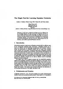
The foundation for the approach of reducing alarm floods by identifying the root cause is the causal model. It is essential to learn a very accurate causal model to identify the causal chain and to determine the root cause. Therefore, it is important to know how a causal model can be learned in an unsupervised way and what information about the plant or process is necessary to include. III. K NOWLEDGE REPRESENTATION So far the state of the art in handling the alarm floods is simple and in strong need of improvement. In general, once the amount of alarms is too high to be handled, the new arriving alarms will be ignored by the operator. This means the amount of alarms is randomly reduced which has a high potential of causing a disaster. Therefore, to improve the handling it is necessary to use all available knowledge to reduce the alarm flood in an intelligent way. Best case scenario would be if only the alarms which hint to the real causes, would be displayed. Therefore, it is a demanding task to identify all required causal relations between alarms [27]. To be able to achieve this, it is necessary to construct a causal model. Probabilistic graphical models are suitable for this use case. They represent in an easy-to-understand way the relationships and their probabilities. All these models are composed of nodes n and edges e. In our use case a node is one alarm. The relations of two alarms (nodes) are represented by edges. For the causal model it is beneficial to include as much knowledge about the system as possible to be close to the reality. There are two extreme ways to achieve a representation such as phenomenological and first principle representation. The first approach is to learn the statistical relations of the alarms based on the alarm logs. However, it does not include every aspect of the plant. For example, as shown in Fig. 1, only the symptoms are presented. Alarm 1

Alarm 2

Alarm 4

Alarm 7

Alarm 3

Alarm 5

Alarm 6

Fig. 1. Phenomenological representation

But the alarms themselves may not be depended directly on each other. It’s more viable to believe, that based on location or process flow the alarms are propagating and have effect on each another. The representation only depicts correlations and not causal relationships. This leads to the second approach. Here a first principle model of the system is built to create an exact image of the system. Not only the symptoms (alarms) are included, but also all aspects such as sensor values see Fig. 2.

Sensor 1

Sensor 3

Sensor 2 Alarm 1 Sensor 4

Sensor 5

Alarm 2

Alarm 3

Fig. 2. First principle representation

This has an advantage of representing a deeper knowledge about the relations between the alarms and how the dependencies are. However, in most cases this is not possible due to missing information about some parts of the plant such as process flow. Also the creation of a model needs an expert and is very time-consuming. Hence, a combination of both is the most favourable solution. The model should include as much knowledge about the plant (process flow, environment etc.) as possible without being too time consuming. Finding a good balance is one of the challenges for researchers. In a best case scenario, the advantages of fast learning from historical data approach can be combined with the valuable expert knowledge about the plant and process. We use a Bayesian network as a data-driven approach and try to fill it with as much information about the plant as possible. The first step into this direction is to evaluate the most suitable method for learning the structure of a Bayesian network. IV. BAYESIAN N ETWORK A PPROACH Bayesian networks are a class of graphical models which allow an intuitive representation of multivariate data. A Bayesian network is a directed acyclic graph, denoted B = (N, E), with a set of variables X = {X1 , X2 , . . . , Xp }. Each node n ∈ N is associated with one variable Xi . The edges e ∈ E, which connect the nodes, represent direct probabilistic dependencies. Abele et al. [23] and Wang et al. [24] have already tried to use Bayesian networks for detection of a root-cause in an alarm flood. Abele et al. learned a Bayesian network, which is consequently the basis for root-cause analysis of a pressure tank system. The structure of the Bayesian network was learned with a constrained-based method and needed some expert knowledge to achieve the correct model of the pressure tank system. Therefore, they conclude that expert knowledge and machine learning should be combined for better results. Wang et al. applied a special kind of Bayesian networks. They restrict themselves to only one-child nodes. This is a huge restriction and it cuts off many possible failure cases, because in a modern and complex industry plant the interconnectivity is increasing dramatically. This means that the alarms are also more connected and dependent on each other. Structure Learning Therefore, we want to pursue the idea of Abele et al. and use the Bayesian network as a model to represent the

causality of the alarms. But other than Abele et al. we do not limit ourselves to constraint-based learning methods. In the following different structure learning algorithms are evaluated. All in all these learning algorithms can be differentiated into the following three groups of methods: • constrained-based, • score-based, • hybrid. In a constrained-based method the Bayesian network is a representation of independencies. The data is tested for conditional dependencies and independencies to identify a structure, which explains the dependencies and independencies of the data the best. Constrained-based methods are susceptible to failures in individual independence tests. Just one wrong answered independence test mislead to a wrong structure. For the evaluation we use the Grow-Shrink (GS) algorithm from D. Magaratis [28]. Score-based methods view Bayesian network as specifying a statistical model. Therefore, it is more like a model selection problem. In the first step, a hypothesis space of potential network structures is defined. In the second step, the potential structures are measured with a scoring function. The scoring function shows how good a potential structure fits the observed data. Following this, the computational task is to identify the highest-scoring structure. This task consists of a superexpo2 nential number of potential structures 2O(n ) . Therefore, it is unsure if the highest-scoring structure can be found, so the algorithms use heuristic search techniques. Because the score-based methods consider the whole structure at once, they are less susceptible to individual failures and better at making compromises between the extent to which variables are dependent in the data and the cost of adding the edge [29]. For the evaluation we use the well-known Hill-Climbing (HC) algorithm. Hybrid methods combine aspects of both constraint-based and score-based methods. They use conditional independence tests to reduce the search space and network scores to find the optimal network in the reduced space at the same time. For the evaluation we use the Max-Min Hill-Climbing Algorithm (MMHC) from Tsamardinos et al. [30]. Demonstrator For the evaluation of these three algorithms, we implemented two simple use cases in the Versatile Production System (VPS), which is located in the SmartFactoryOWL. The VPS is a manufacturing plant in a laboratory scale where sensors, actuators, bus systems, automation components, and software from different manufacturers are considered. The VPS is a hybrid technical process considering both continuous and discrete process elements with a focus on the information processes and communication technologies from the plant level down to the sensor level. It thus provides an ideal multi vendor platform for testing and validation of innovative technologies and products. The use cases are implemented in the ”bottle filling module” of the VPS. The bottles can be filled either with water or with

grain. The two use cases represent two possible root causes for an alarm flood. We want to identify these root causes with correctly learnt dependencies of alarms. In Fig. 3 an overview of the ”bottle filling module” is depicted. Start area / collection area of bottles

Algorithms

Conveyor belt Grain filling

Water filling

2

3

1

4

Put the cap on

Caps

Rotary table Claw

5

6

Screw the cap

Claw

Camera

The two root causes for an alarm flood are bottle rotary table entrance (BRE) and drive filling (DF). If a bottle is missing the alarm BRE triggers. This alarm causes the subsequent alarms TW, TF, TC1, TC2, and BNF. In the other root cause of a blocked drive the alarm DF causes the subsequent alarms TF, TC1, TC2, and BNF.

= Stations Conveyor belt

In the following, the three algorithm Grow-Shrink (GS), Hill-Climbing (HC), and Max-Min Hill-Climbing (MMHC) are presented and evaluated. D. Magaratis developed the GS algorithm [28]. For the understanding of the algorithm some definitions are necessary. Hence, a Bayesian network is abbreviated with B and its structure with S. The set of potential nodes U consists of nodes X1 , . . . , Xi and nodes Y1 , . . . , Yj . The nodes X represent the nodes which are already part of the structure and Y are new potential nodes which are not part of the structure. The algorithm can be divided into two phases, a growing phase and a shrinking phase. In the growing phase new nodes are added to the current structure and in the shrinking phase redundant nodes will be removed. The pseudo code of GS looks as follows:

Fig. 3. Overview bottle filling module

The module consists of a conveyor belt and a rotary table with six stations. At the first station the bottle is handed over by the conveyor belt to the rotary table. It’s possible to fill the bottle either with water at station two or to fill it with grain at station three. The next two stations are there for putting the cap on. At the first step, the cap is placed on top of the bottle and in the second step, the cap is fastened. In the last station the bottle is handed over back to the conveyor belt passing a camera check, whether the bottle is filled. In total the following alarms are implemented: bottle rotary table entrance (BRE), timer water tank (TW), drive filling (DF), timer filling (TF), timer cap 1 (TC1), timer cap 2 (TC2), bottle not filled (BNF). The real dependencies between the alarms are depicted in Fig. 4. This structure shows the real causality within the plant. Bottle rotary table entrance (BRE)

Timer water tank (TW)

Drive filling (DF)

Algorithm 1 Grow-Shrink 1: S ← 0 Growing Phase: 2: While ∃Y ∈ U − {Y } such that Y ⊥ 6 X | S , do S ← S ∪ {Y } Shrinking Phase: 3: While ∃Y ∈ S such that Y ⊥ X | S − {Y }, do S ← S − {Y } 4: B (X) ← S . The algorithm starts with an empty structure S. The growing phase adds variables Y from a set of U as long as they are dependent on X, given the current structure S. This process continues until there are no more variables Y left. There may be some variables that were added to S which became independent from X at a later point. This initiates the shrinking phase which identifies and removes these variables. Based on a training dataset, the GS algorithm learned the following structure, which is depicted in Fig. 5.

Timer filling (TF)

TW DF

BRE

Timer cap 1 (TC1)

TF

Timer cap 2 (TC2)

Bottle not filled (BNF)

Fig. 4. Real causality structure

BNF

TC1

TC2

Fig. 5. BN Grow-Shrink

The result of the GS algorithm is an undirected Bayesian network. All edges, which are also in the real causal model,

are learned. Unfortunately there are two false connections in the structure. Both the edges BRE and DF as well as the edge between TW and DF are incorrect. But in general, this algorithm is well suited to serve as a basis for a combination of the model with expert knowledge to achieve an accurate model. The Hill-Climbing (HC) algorithm belongs to the score-based approaches. The algorithm enjoys great popularity because of its speed and ease of implementation. The algorithm tries to improve the score of the Bayesian network with one transition, namely add or remove an edge or a node. If the algorithm cannot find a transition to improve, it stops. This has the potential danger of a local maximum in the score for the Bayesian network. For a better understanding of the pseudo code we define some variables. The Bayesian network B consists of a set of nodes U and a set of edges E. The set of nodes U contains the variables X = {X1 , . . . , Xi } and Y = {Y1 , . . . , Yj }. The variable score is the score of the Bayesian network. The highest score during the algorithm is saved in the variable maxscore. The scores are calculated with a ScoreFunction like Bayesian information criterion (BIC). The ScoreFunction determines how well the Bayesian network B fits to the given data D. The pseudo code of HC looks as follows: Algorithm 2 Hill-Climbing 1: B ← (U, E) 2: score ← −∞ 3: do: 4: maxscore ← score 5: for each attribute pair (X, Y ) do 6: for each E 0 ∈ {E ∪ {X → Y }}, E 0 ∈ {E − {X → Y }}, E 0 ∈ {E − {X → Y } ∪ {Y → X}}, 0 0 7: B ← (U , E 0 ) 8: newscore ← ScoreF unction(B 0 , D) 9: if newscore > score then B ← B0 score ← newscore 10: end if 11: end for 12: while score > maxscore 13: return B The HC algorithm starts with a Bayesian network which consists of nodes U and edges E. For the start, the structure has zero edges and a score of minus infinity, which symbolise the worst score possible. In the following, the algorithm tries to improve the score by either adding, removing, or reversing an edge between X and Y . After each of this actions the new score is calculated and scored. The score is based on how well the Bayesian network fits the data D. If the algorithm is unable to find one transition to improve the score further it ends and returns the structure of the Bayesian network. Based on the training dataset the HC algorithm gives the following structure, which is depicted in Fig. 6.

TW DF

BRE

TF

BNF

TC1

TC2

Fig. 6. BN Hill-Climbing

The result is a directed Bayesian network. The use case of a blocked drive for the grain filling is correctly represented (DF → TF → TC1 → TC2 → BNF). Unfortunately, likewise the GS algorithm, some connections are incorrectly learned, namely DF → BRE and TF → BRE. Also the orientation of the edge between TW and TF is false. All in all, this algorithm also provides a good foundation to achieve an accurate model when combined with expert knowledge. The last algorithm we want to evaluate for learning a causal model is the Max-Min Hill-Climbing (MMHC) algorithm, which was developed by Tsamardinos et al. [30]. This algorithm is a hybrid of a constrained-based and score-based approach. In the first step, the search space for children and parents nodes is reduced by using a constrained-based approach, namely Max-Min Parents and Children (MMPC) algorithm. In the second step, the Hill-Climbing algorithm is applied to find the best fitting structure from the reduced search space. For a better understanding of the associated pseudo code, we need a few definitions. The dataset D consists of a set of variables ϑ. In the variable P Cx the candidates of parents and children for the node X are stored. This set of candidates is calculated with MMPC algorithm. The variable Y is a node of the set P Cx . The pseudo code of MMHC looks as follows: Algorithm 3 MMHC Algorithm 1: procedure MMHC(D) 2: Input: data D 3: Output: a DAG on the variables in D 4: % Restrict 5: for every variable X ∈ ϑ do 6: P CX = MMPC(X, D) 7: end for 8: % Search 9: Starting from an empty graph perform Greedy HillClimbing with operators add-edge, delete-edge, reverseedge. Y → X if Y ∈ P CX 10: Return the highest scoring DAG found 11: end procedure The algorithm first identifies the parents and children set of each variable, then performs a greedy Hill-Climbing search in the reduced space of Bayesian network. The search begins with an empty graph. The edge addition, removal, or reversing which leads to the largest increase in the score is taken and the search continues in a similar way recursively. The difference

from standard Hill-Climbing is that the search is constrained to only consider edges which where discovered by MMPC in the first phase. The MMPC algorithm calculates the correlation between the nodes. Based on the training dataset the MMHC algorithm gives the structure which is depicted in Fig. 7. TW DF

BRE

TF

BNF

TC1

TC2

Fig. 7. BN Max-Min Hill-Climbing

The result is very close to the true causal model in Fig. 4. Both, the use-case with the missing bottle (BRE → TW → TF → TC1 → TC2 → FNB) and the use-case with the blocked drive (DF → TF → TC1 → TC2 → FNB) are shown correctly. Only the connection between DF and BRE is not present in reality. Evaluation

which is a combination of a constrained-based method and a score-based method, shows the best performance. This leaves only HC with one incorrectly learned orientation. A different picture is shown, if we take a look at the number of tests and the average runtime of the algorithms. The test includes both conditional independence tests and calls of the scoring function. The constrained-based method GS needs 92 conditional independence tests. The HC algorithm calls the scoring function 69 times and the MMHC algorithm 77 times. The number of test is an indicator for the execution time but they are not strictly proportional. Different implementations may use different data structures for performing graph operations and also the duration of a test depends on the the size of the conditioning set or parent set. Therefore, the average runtime is also depicted. The fastest algorithm is, as expected, the HC algorithm with 4.15 ms, followed by the GS algorithm with 6.45 ms and the MMHC algorithm with 9.95 ms. This result is expected, because the MMHC algorithm is a combination of an constraint-based and score-based method. However, it has to be considered, that in a world like today the bottleneck is not the calculation power. The accuracy of the structure is way more important. V. C ONCLUSION

In the following subsection, the results of the three different algorithms are compared. In the previous subsection it was shown, that all algorithms led to a decent structure, which can serve as a foundation. Together with time-limited expert knowledge an accurate causal model can be achieved. Abele et al. restricted themselves to constrained-based algorithms for learning the structure of an Bayesian network. The evaluation of different learning methods on the versatile production system shows that this restriction is unjustified. The results of the evaluation are depicted in detail in Table I TABLE I R ESULTS OF EVALUATION

Amount of edges Correct edges Incorrect edges Correct orientation Incorrect orientation Number of tests Mean runtime [ms]

GS

HC

MMHC

8 6 2 92 6.45

8 6 2 5 1 69 4.15

7 6 1 6 77 9.95

The amount of edges are the same between GS and HC. The MMHC algorithms proves here to be a better fit. All algorithms are able to learn the six correct edges. The GS and HC algorithms have two incorrectly learned edges. Here the MMHC algorithm is also ahead with just one false edge. The same applies to the orientation of the edges. Only the HC and the MMHC algorithms could learn the orientation of edges. While MMHC can also score here with all six edges correctly orientated, the HC algorithm is only able to identify five of the six orientations correctly. In general, the MMHC algorithm,

We presented the increasing problem of overwhelming alarm floods in industrial plants. One way to solve this problem is to reduce the alarm floods, especially sequences of alarms caused by one alarm. Therefore, we propose to identify the real root cause of an alarm flood using Bayesian networks. The Bayesian network serves as a causal model and enables inference about the root cause. Instead of all alarms, only the root cause is depicted to the operator. This supports the operator to take better care of the plant. The foundation for this approach is the structure of the Bayesian network. Therefore, we evaluated respectively one algorithm from the three different methods: constrained-based, score-based, and hybrid. The evaluation has shown that a restriction to only constrainedbased methods is unjustified. We achieved better results in the form of accuracy with a hybrid method. A disadvantage is a longer computation time. Nevertheless, we think that Bayesian networks are a good foundation to learn a causal model of the dependencies of alarms in a plant. Bayesian networks are robust against uncertainty such as incomplete or defective data. Because it’s a data-driven approach it reduces the amount of time in which an expert is needed for constructing the causal model. The expert knowledge is still necessary, but the approach with Bayesian network can be improved by including time behaviour or dynamic process like a product change in the plant. Also the algorithms for learning the structure can be improved by using methods like Transfer Entropy for a better edge orientation. ACKNOWLEDGMENT The work was supported by the German Federal Ministry of Education and Research (BMBF) under the project ADIMA (funding code: 03FH019PX5).

R EFERENCES [1] B. Hollifield, E. Habibi, and J. Pinto, The Alarm Management Handbook: A Comprehensive Guide. PAS, 2010. [2] D. Rothenberg, Alarm Management for Process Control: A Best-practice Guide for Design, Implementation, and Use of Industrial Alarm Systems. Momentum Press, 2009. ¨ [3] J. E. Larsson, B. Ohman, A. Calzada, and J. DeBor, “New solutions for alarm problems,” in Proceedings of the 5th International Topical Meeting on Nuclear Plant Instrumentation, Controls, and Human Interface Technology, Albuquerque, New Mexico, 2006. [4] J. Wang, F. Yang, T. Chen, and S. L. Shah, “An overview of industrial alarm systems: Main causes for alarm overloading, research status, and open problems,” IEEE Transactions on Automation Science and Engineering, vol. 13, no. 2, pp. 1045–1061, April 2016. [5] P. T. Bullemer, M. Tolsma, D. Reising, and J. Laberge, “Towards improving operator alarm flood responses: Alternative alarm presentation techniques,” Abnormal Situation Management Consortium, 2011. [6] M. Hollender, T. C. Skovholt, and J. Evans, “Holistic alarm management throughout the plant lifecycle,” in 2016 Petroleum and Chemical Industry Conference Europe (PCIC Europe), June 2016, pp. 1–6. [7] G. B. Health and S. Executive, The Explosion and Fires at the Texaco Refinery, Milford Haven, 24 July 1994: A Report of the Investigation by the Health and Safety Executive Into the Explosion and Fires on the Pembroke Cracking Company Plant at the Texaco Refinery, Milford Haven on 24 July 1994, ser. Incident Report Series. HSE Books, 1997. [8] L. M. Toth, A. C. Society., and A. C. Society., The Three Mile Island accident : diagnosis and prognosis / L.M. Toth ... [et al.], editors. American Chemical Society Washington, D.C, 1986. [9] U.-C. P. S. O. T. Force, Final Report on the August 14, 2003 Blackout in the United States and Canada: Causes and Recommendations. Natural Resources Canada, 2004. [10] U. S. N. C. on the BP Deepwater Horizon Oil Spill and O. Drilling, Deep Water: The Gulf Oil Disaster and the Future of Offshore Drilling : Recommendations. National Commission on the BP Deepwater Horizon Oil Spill and Offshore Drilling, 2011. [11] E. Equipment, M. U. Association, E. Equipment, and M. U. A. Staff, Alarm Systems: A Guide to Design, Management and Procurement, ser. EEMUA publication. EEMUA (Engineering Equipment & Materials Users Association), 2007. [12] M. Bransby and J. Jenkinson, The management of alarm systems. Citeseer, 1998. [13] I. S. of Automation and A. N. S. Institute, ANSI/ISA-18.2-2009, Management of Alarm Systems for the Process Industries. ISA, 2009. [14] I. E. Commission, “En-iec 62682:2014 management of alarm systems for the process industries,” International Electrotechnical Commission, Tech. Rep. [15] M. Bransby, “Design of alarm systems,” IEE CONTROL ENGINEERING SERIES, pp. 207–221, 2001. [16] P. Urban and L. Landryov, “Identification and evaluation of alarm logs from the alarm management system,” in 2016 17th International Carpathian Control Conference (ICCC), May 2016, pp. 769–774. [17] N. P. Directorate, “Principles for alarm system design,” YA-711, Feb, 2001. [18] M. Kezunovic and Y. Guan, “Intelligent alarm processing: From data intensive to information rich,” in 2009 42nd Hawaii International Conference on System Sciences, Jan 2009, pp. 1–8. [19] Z. Simeu-Abazi, A. Lefebvre, and J.-P. Derain, “A methodology of alarm filtering using dynamic fault tree,” Reliability Engineering & System Safety, vol. 96, no. 2, pp. 257 – 266, 2011. [20] W. Guo, F. Wen, Z. Liao, L. Wei, and J. Xin, “An analytic modelbased approach for power system alarm processing employing temporal constraint network,” IEEE Transactions on Power Delivery, vol. 25, no. 4, pp. 2435–2447, Oct 2010. [21] L. Wei, W. Guo, F. Wen, G. Ledwich, Z. Liao, and J. Xin, “An online intelligent alarm-processing system for digital substations,” IEEE Transactions on Power Delivery, vol. 26, no. 3, pp. 1615–1624, July 2011. [22] J. Wang, H. Li, J. Huang, and C. Su, “Association rules mining based analysis of consequential alarm sequences in chemical processes,” Journal of Loss Prevention in the Process Industries, vol. 41, pp. 178 – 185, 2016.

[23] L. Abele, M. Anic, T. Gutmann, J. Folmer, M. Kleinsteuber, and B. Vogel-Heuser, “Combining knowledge modeling and machine learning for alarm root cause analysis,” IFAC Proceedings Volumes, vol. 46, no. 9, pp. 1843 – 1848, 2013. [24] J. Wang, J. Xu, and D. Zhu, “Online root-cause analysis of alarms in discrete bayesian networks with known structures,” in Proceeding of the 11th World Congress on Intelligent Control and Automation, June 2014, pp. 467–472. [25] L. Dubois, J.-M. Fort, P. Mack, and L. Ryckaert, “Advanced logic for alarm and event processing: Methods to reduce cognitive load for control room operators,” IFAC Proceedings Volumes, vol. 43, no. 13, pp. 158 – 163, 2010. [26] J.-W. Lee, J.-T. Kim, J.-C. Park, I.-K. Hwang, and S.-P. Lyu, “Computerbased alarm processing and presentation methods in nuclear power plants,” World academy of science, engineering and technology, 2010. [27] M. Hollender and C. Beuthel, “Intelligent alarming,” ABB review, vol. 1, pp. 20–23, 2007. [28] D. Margaritis, “Learning bayesian network model structure from data,” Tech. Rep., 2003. [29] D. Koller and N. Friedman, Probabilistic Graphical Models: Principles and Techniques - Adaptive Computation and Machine Learning. The MIT Press, 2009. [30] I. Tsamardinos, L. E. Brown, and C. F. Aliferis, “The max-min hill-climbing bayesian network structure learning algorithm,” Machine Learning, vol. 65, no. 1, pp. 31–78, 2006.