Study for online range monitoring with the Interaction ...

Physics in Medicine and Biology

ACCEPTED MANUSCRIPT

Study for online range monitoring with the Interaction Vertex Imaging method To cite this article before publication: Christian Finck et al 2017 Phys. Med. Biol. in press https://doi.org/10.1088/1361-6560/aa954e

Manuscript version: Accepted Manuscript Accepted Manuscript is “the version of the article accepted for publication including all changes made as a result of the peer review process, and which may also include the addition to the article by IOP Publishing of a header, an article ID, a cover sheet and/or an ‘Accepted Manuscript’ watermark, but excluding any other editing, typesetting or other changes made by IOP Publishing and/or its licensors” This Accepted Manuscript is © 2017 Institute of Physics and Engineering in Medicine.

During the embargo period (the 12 month period from the publication of the Version of Record of this article), the Accepted Manuscript is fully protected by copyright and cannot be reused or reposted elsewhere. As the Version of Record of this article is going to be / has been published on a subscription basis, this Accepted Manuscript is available for reuse under a CC BY-NC-ND 3.0 licence after the 12 month embargo period. After the embargo period, everyone is permitted to use copy and redistribute this article for non-commercial purposes only, provided that they adhere to all the terms of the licence https://creativecommons.org/licences/by-nc-nd/3.0 Although reasonable endeavours have been taken to obtain all necessary permissions from third parties to include their copyrighted content within this article, their full citation and copyright line may not be present in this Accepted Manuscript version. Before using any content from this article, please refer to the Version of Record on IOPscience once published for full citation and copyright details, as permissions will likely be required. All third party content is fully copyright protected, unless specifically stated otherwise in the figure caption in the Version of Record. View the article online for updates and enhancements.

This content was downloaded from IP address 130.79.168.107 on 24/10/2017 at 07:51

us cri

Study for online range monitoring with the Interaction Vertex Imaging method

Ch. Finck1 , Y. Karakaya1 , V. Reithinger2 , R. Rescigno1 , J. Baudot1 , J. Constanzo1 , D. Juliani1 , J. Krimmer2 , I. Rinaldi3 ‡ , M. Rousseau1 , E. Testa2 , M. Vanstalle1 and C. Ray2 § 1

an

Université de Strasbourg, CNRS, IPHC UMR 7871, F-67000 STRASBOURG, France 2 Institut de Physique Nucléaire de Lyon, Université de Lyon, 69003 Villeurbanne, France, IN2P3/CNRS, UMR5822, Université de Lyon 1, 69622 Villeurbanne, France 3 Department of Radiation Oncology, Heidelberg University Clinic, Heidelberg, Germany E-mail: [email protected]

ce

pte

dM

Abstract. Ion beam therapy enables a highly accurate dose conformation delivery to the tumor due to the finite range of charged ions in matter (i.e., Bragg Peak (BP)). Consequently, the dose profile is very sensitive to patients anatomical changes as well as minor mispositioning, and so it requires improved dose control techniques. Proton Interaction Vertex Imaging (IVI) could offer an online range control in carbon ion therapy. In this paper, a statistical method was used to study the sensitivity of the IVI technique on experimental data obtained from the Heidelberg Ion-Beam Therapy Center. The vertices of secondary protons were reconstructed with pixelized silicon detectors. The statistical study used the χ2 test of the reconstructed vertex distributions for a given displacement of the BP position as a function of the impinging carbon ions. Different phantom configurations were used with or without bone equivalent tissue and air inserts. The inflection points in the fall-off region of the longitudinal vertex distribution were computed using different methods, while the relation with the BP position was established. In the present setup, the resolution of the BP position was about 4-5 mm in the homogeneous phantom under clinical conditions (106 incident carbon ions). Our results show that the IVI method could therefore monitor the BP position with a promising resolution in clinical conditions.

Ac

1 2 3 4 5 6 7 8 9 10 11 12 13 14 15 16 17 18 19 20 21 22 23 24 25 26 27 28 29 30 31 32 33 34 35 36 37 38 39 40 41 42 43 44 45 46 47 48 49 50 51 52 53 54 55 56 57 58 59 60

AUTHOR SUBMITTED MANUSCRIPT - PMB-105774.R2

pt

Page 1 of 23

Submitted to: Phys. Med. Biol.

‡ current address: Institut de Physique Nucléaire de Lyon, Université de Lyon, 69003 Villeurbanne, France, IN2P3/CNRS, UMR5822, Université de Lyon 1, 69622 Villeurbanne, France § current address: Institut Lumière Matière, Université de Lyon, 69622 Villeurbanne, France, CNRS, Université de Lyon 1, 69622 Villeurbanne France


2

pt

Study for online range monitoring with the Interaction Vertex Imaging method 1. Introduction

ce

pte

dM

an

us cri

The use of charged ion beams in cancer therapy is motivated by the highly sharp dose distribution at the end of their range, notably the Bragg Peak (BP). Charged particles heavier than protons (e.g., 12 C) have additional advantages including reduced lateral scattering and an increased relative biological effectiveness mainly in the BP region. Ions are therefore well suited to the treatment of deeply located radioresistant tumors (Schardt et al 2010). In terms of the increased energy deposition in the BP region it is crucial to accurately deliver the dose to the tumor. Indeed, range uncertainty of just few millimeters can lead to an under-dosage in the target volume or an overdosage in the organs at risk. Several patient-related uncertainties can influence the particle range: conversion of X-ray computed tomography image to relative ion stopping power for treatment planning (Paganetti 2012, Woodward et al 2016), patient mispositioning, morphological changes of the tumor over the treatment course and organ motion (Thomas 2006). To overcome these uncertainties, additional safety margins of about 3-5 mm are required to ensure the local control of the tumor (McGowan et al 2013). To reduce margins, online monitoring of the ion range is desirable. Several techniques have been studied based on the detection of secondary particles produced during nuclear reactions, such as 11 C, 10 C and 15 O, along with positron emissions. Positron emission tomography (PET) was used in-beam at the Helmholtz Centre for Heavy Ion Research (GSI) treatment facility until 2008 to control the delivery of carbon ion therapy (Enghardt et al 2004, Parodi et al 2008). More recently in-beam PET was tested with clinical proton beams (Piliero et al 2015) and clinical carbon beams (Gianoli et al 2017). Nevertheless, the half-life of the radioactive nuclei limits this method due to low signals and biological washout (Parodi et al 2008a, Fiedler et al 2008, Helmbrecht et al 2013). To overcome these problems an online PET was studied, although reconstruction methods demonstrated a prompt-γ contamination (Enghardt et al 2004, Knopf et al 2009). The prompt-γ emitted during nuclear reactions can also be used for range monitoring by reconstructing the emission points. The emission profile of prompt-γ rays along the ion path was found to be correlated with the primary ion range both for protons (Min et al 2006) and carbon ions (Testa et al 2008, Testa et al 2009). The quasi-instantaneous emission of prompt-γ could lead to a real online range control (Testa et al 2010, Moteabbed et al 2011). A prototype of a knife-edge slit camera was thus used to measure of prompt-γ profiles in inhomogeneous targets, during proton irradiation. Range deviations were detected within less than 2 mm in most of the cases (Priegnitz et al 2015). A third modality, known as Interaction Vertex Imaging (IVI), was proposed by (Amaldi et al 2010) for carbon-ion-therapy range monitoring. This method, based on the detection of secondary particles to reconstruct the nuclear emission vertices, has been studied in both simulations (Henriquet et al 2012) and experiments (Gwosch et

Ac

1 2 3 4 5 6 7 8 9 10 11 12 13 14 15 16 17 18 19 20 21 22 23 24 25 26 27 28 29 30 31 32 33 34 35 36 37 38 39 40 41 42 43 44 45 46 47 48 49 50 51 52 53 54 55 56 57 58 59 60

Page 2 of 23

Page 3 of 23

3

pt


pte

dM

an

us cri

al 2013, Piersanti et al 2014). The range of the primary beam can be monitored with a precision of few millimeters, typically 1-3 mm (Gwosch et al 2013). Any fragments leaving the patient, mainly comprising protons and α particles, can be detected using a dedicated tracking device. IVI monitoring aims to detect deviations in the delivered range using measured emission vertex profiles (Henriquet et al 2012). Methods have been proposed to compute the BP positions based on the vertex distributions of secondary charged particle tracks. In the paper (Henriquet et al 2012), the authors used a tracker based on pixelized Complementary-Metal-Oxide-Semiconductor (CMOS) sensors, while in (Gwosch et al 2013) a hybrid-pixel detector with a CMOS readout chip was used. In both cases the tracker was placed downstream from the phantom at an angle of ∼30° with respect to the beam axis. The sensors presented a good spatial resolution (< 10 µm) with a thin layer of silicon, being 50 µm and 300 µm in the two studies, respectively, which reduced the material budget. A setup combining the three modalities was proposed in (Marafini et al 2015). Since this profile is correlated to the BP position, discrepancies in the vertex distributions highlight a difference between the predicted and measured BP position (∆BP). The ability to detect this deviation depends on ∆BP values and the statistic used to build the longitudinal vertex distributions. Given the high spatial resolution of the CMOS detector, the deviation is not affected by the track reconstruction method. In our study, the sensitivity of the IVI method was evaluated as a function of the number of incident carbon ions at the Heidelberg Ion-beam Therapy (HIT) clinical center as part of the Quality Assurance by Protons Interaction Vertex Imaging (QAPIVI) project. The tracking device used to reconstruct the secondary particle tracks was based on CMOS technology. A statistical approach based on the χ2 test, (e.g., (Gagunashvili 2005)), was applied on the collected data to determine the minimum number of incident carbon ions ˜12C ) necessary to disentangle two different vertex distributions for a given ∆BP. (N In our paper, we first describe the optimization of the tracking device position (azimuthal angle and distance to the phantom center) by means of simulations. We then present the results of the χ2 test applied to the experimental data.

ce

2. Methods and materials 2.1. Experimental setup

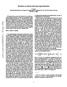
Measurements were performed at HIT. The experimental setup consisted of a tracking device placed downstream from the phantom at a given angle (θ) with respect to the beam axis, as shown in Figure 1.

Ac

1 2 3 4 5 6 7 8 9 10 11 12 13 14 15 16 17 18 19 20 21 22 23 24 25 26 27 28 29 30 31 32 33 34 35 36 37 38 39 40 41 42 43 44 45 46 47 48 49 50 51 52 53 54 55 56 57 58 59 60


2.1.1. Beam: the energy of the carbon ions ranged from 240 MeV/u to 310 MeV/u. The beam had a Gaussian shape with a FWHM of 4.2 mm. The beam delivery involved an active scanning system with total spill length of 9 seconds. The total number of carbon ions per spill was around 24 × 106 .


Y

28m

m

Beam

us cri

Phantom (0,0,0)

90mm

4

pt


Track e

θ

x

r

Z

50m

160mm

m

an

Figure 1. Schematic view of the experimental setup, with the cylindrical phantom with the five inserts and the four planes of CMOS sensors. The inserts of different media labelled 1 to 5 were placed at 40, 80, 120, 20 and 140 mm respectively from the phantom entrance. The beam was along the Z axis.

ce

pte

dM

2.1.2. Cylindrical phantom: the cylindrical phantom was made of PolyMethyl MethAcrylate (PMMA) with a density of 1.19. The size was comparable to a human head (diameter: 160 mm, height: 90 mm) with five cylindrical holes (diameter: 28 mm) in which rods of various materials can be inserted. Holes were made in Y directions, and the center-to-center distance was 40 mm for inserts labelled 1 and 3 and 60 mm for inserts labelled 4 and 5. Insert 2 was positioned at the phantom center, insert 4 was located closest to the phantom entrance (upstream) only 6 mm from the edge, while insert 3 was closest to the end of the phantom (downstream), at a distance of 26 mm from the edge (Figure 1). The phantom could be rotated ±90° around the Y axis to select a given insert. Three different insert materials were used, namely PMMA, air, with a density of 1.29×10−3 , and cortical bone-equivalent tissue, with a density of 1.85. The latter was composed of 44.6 % of oxygen, 21 % of calcium, 14.4 % of carbon, 10 % of phosphorus, 4.7 % of hydrogen, 4.2 % of nitrogen, 0.3 % of sulfur, 0.2 % of magnesium and 0.01 % of zinc. Hereafter the cortical bone-equivalent material will simply be referred to as bone. Five different configurations were used for the phantom: • Config1: the homogenous phantom, with all inserts made of PMMA material; • Config2a: an air insert located at the different positions, namely positions labelled from 1 to 4 in the phantom;

Ac

1 2 3 4 5 6 7 8 9 10 11 12 13 14 15 16 17 18 19 20 21 22 23 24 25 26 27 28 29 30 31 32 33 34 35 36 37 38 39 40 41 42 43 44 45 46 47 48 49 50 51 52 53 54 55 56 57 58 59 60

Page 4 of 23

• Config2b: a bone insert located at the different positions labelled from 1 to 4 in the phantom; • Config3a: an air insert located at position 3 (downstream) in the phantom;

• Config3b: a bone insert located at position 2 in the phantom.

Page 5 of 23

5

pt


dM

an

us cri

2.1.3. Tracking device: the tracking device consisted of four planes of two MIMOSA26 (M26) CMOS sensors (Hu-Guo et al 2010). Each plane had two sensors overlapping in a region of 100 µm. The sensor planes were placed in two different aluminum boxes in pairs. The boxes had a width and a height of 20 cm and a depth of 2.5 cm. Windows, larger than the active area of the sensors, were located on each side of the box. The two boxes were fixed on an arm allowing for rotation at different angle settings relative to the beam axis. The precision of the angle setting was about 0.5°. The distance between the two boxes was 5 cm, while the distance between the two consecutive planes was 5 mm. The M26 chip had a sensitive area of 10.6×20.2 mm2 and was covered by 576 rows and 1152 columns of pixels with 18.4 µm pitch. A pixel was considered as fired when the deposited charge was above the threshold set at 8 times the noise level (which was about 13-14 electrons). The columns were read out in a rolling shutter mode with an integration time of 115.2 µs (i.e., frequency of 87 kHz) without any dead-time. The collected data were formatted on the PXI crate controller and stored on a local hardware disk. The tracking device was placed at θ = 10° with respect to axis beam for all aforementioned configurations. This angle was chosen after performing optimization simulations. This optimization will be presented below. 2.2. Analysis software and simulation

ce

pte

The reconstruction software associated with the tracking device was previously described (Topi et al 2016). The fired pixels corresponding to a single particle were identified for each plane; clusters compatible with a straight trajectory were then matched to reconstruct the particle tracks (tracking); finally, the vertex position (vertexing) was computed. The vertex position was defined as the center of the minimal distance between the beam position and the secondary proton track. The performance of the reconstruction algorithms was assessed using of Monte-Carlo (MC) simulation with a 8 mm thick carbon target. An efficiency of 99% was found both for tracking and vertexing algorithms. The resolution of the vertex distribution was around 11 µm in X and Y directions and less than 60 µm in the longitudinal direction (i.e., beam axis) (Rescigno et al 2014). These results were obtained with the compact geometry of the vertex device. The distance between two consecutive planes of the tracking device was of 3 mm. In these conditions the angular coverage was of ±40° (Topi et al 2016). Furthermore, a simulation package, based on GEANT4 10.01 (Agostinelli et al 2003), was developed to model the entire experimental setup. The Bertini physics list is suitable for energies less than 10 GeV (Wright et al 2015), while the Binary Cascade light ion model (BIC), described in (Folger et al 2004), is more suitable for low energy physics (< 200 MeV/u). Regardless of whether the Bertini physics list or BIC was used, the production rate of the simulated vertices compared to the experimental ones was 1.5 to 2 times higher depending on the carbon ion energy. By contrast, the simulated and experimental vertex distributions had a similar shape, especially in the fall-off region. Indeed the p-value of the χ2 test was 0.86 ± 0.03. In the following, the Bertini list was

Ac

1 2 3 4 5 6 7 8 9 10 11 12 13 14 15 16 17 18 19 20 21 22 23 24 25 26 27 28 29 30 31 32 33 34 35 36 37 38 39 40 41 42 43 44 45 46 47 48 49 50 51 52 53 54 55 56 57 58 59 60



6

pt


dM

2.3. The χ2 test method

an

us cri

used for the simulated data. The width and position of the beam impinging on the phantom as well as the number of fired pixels versus deposited energy in the CMOS sensor were included in the simulation. A phenomenological model was implemented to determine the deposited charge in each pixel (Rescigno et al 2014). The noise pattern from electrons hitting the planes and the residual misalignment of the tracker were also included in the simulation. For each simulation, 10 million carbon ions were generated and the corresponding secondary vertices were reconstructed. The resolution of the reconstructed longitudinal vertex positions was estimated by using the residual distribution which is the difference between the vertex position given by the simulation, ztrue , and the reconstructed vertex position, zrec . This resolution σ was determined by applying a Gaussian fit to the residual distributions. In case of a non-Gaussian shape distributions, the RMS values were considered instead. The uncertainties related to the intrinsic vertex resolution were defined as the ratio between vertex resolution (σ or RMS) and the square root of the vertex number (N). This ratio was referred to as variance and labelled as Vσ and VRM S respectively.

ce

pte

For a given acquisition run, each spill was considered as a statistically independent set. Therefore it was possible to combine the spill from one run with the spill from an associated run for a given ∆BP. In this way a statistical χ2 test of consistency was computed for each associated pair of vertex profiles. The two distributions were statistically distinguishable at a level of two standard deviations when the probability (p-value) of the χ2 test was less than 5 %, which depended directly on the number of reconstructed vertices. The choice of the histogram bin size can be a critical issue for the χ2 test. Several methods exist in the literature to define the optimal bin size, as pointed out in (Sturges 1926), (Doane 1976) or (Scott 1979). In our study, the cumulative distribution of vertex profiles was preferred when performing the χ2 test. Indeed, the cumulative distribution is an isomorphic transformation that retains the information of the vertex distribution and drastically reduces the sensitivity of the choice of bin size. The χ2 test was performed only above a certain position for longitudinal vertex position where the two distributions began to differentiate. For a given ∆BP, the pvalues were computed for the vertex distribution obtained for the different spills as a function of the number of incident carbon ions, ranging from 0.5 to 10 millions ˜12C required to at increments of 0.5 million. The minimum number of carbon ions N disentangle two distributions was defined as the crossing point with the p-value = 5 % level.

Ac

1 2 3 4 5 6 7 8 9 10 11 12 13 14 15 16 17 18 19 20 21 22 23 24 25 26 27 28 29 30 31 32 33 34 35 36 37 38 39 40 41 42 43 44 45 46 47 48 49 50 51 52 53 54 55 56 57 58 59 60

Page 6 of 23

2.3.1. χ2 test for Config1: to probe the sensitivity of the IVI method to displacements of the BP position in homogeneous phantom, the χ2 test was first applied to the data

Page 7 of 23

7

pt


us cri

collected with carbon ions impinging on the phantom in Config1. Runs were made at six different energies, ranging from 293.5 MeV/u to 297.8 MeV/u, referred to as High Energies (HE). Six other runs were performed at lower energies ranging from 240.6 MeV/u to 245.4 MeV/u, referred to as Low Energies (LE) (see Table 1, first part). Energies were chosen to ensure a given displacement of the BP position (∆BP). The run with the highest energy was taken as the reference in each case, referred to as run H05 and run L05 for HE and LE data respectively. For HE runs, the lower limit of the depth in the phantom, used in the χ2 test, was set at 80 mm, and below this value, distributions were similar at the 1 ‰ level. The longitudinal vertex position at 80 mm was about 60 mm distance from the BP position (BP: ∼140 mm). For the LE runs, the lower limit was set at 20 mm corresponding to a distance to the BP of ∼80 mm (BP: ∼100 mm). The difference in the lower limits was due to a variation in the BP position.

pte

dM

an

2.3.2. χ2 test for Config2: to probe the sensitivity of the IVI method with regard to insert position, the p-values were computed for Config2b at a beam energy of 308.6 MeV/u and for Config2a at a beam energy of 259.3 MeV/u. H01 and H03 runs, which were taken as reference, had the same BP position as those with the bone and air inserts. These runs were respectively labelled as bone insert position runs and air insert position runs (see Table 1, second part). For these runs, the χ2 test was applied over the full vertex range. As the difference in cumulated vertex distribution of the air insert runs compared to the H03 reference run was large, the p-values were too small to be meaningful, and so the χ2 test over the number of degrees of freedom (NdF) was preferred. Therefore, the higher the χ2 /NdF value, the less similar the vertex distributions. The p-value of 5 % corresponded, in our case, to a value χ2 /NdF of ∼1.2. Above this limit, the vertex distributions were statistically distinguishable at a level of two standard deviations.

ce

2.3.3. χ2 test for Config3: finally, the sensitivity of the IVI method of a BP displacement with a heterogeneous phantom was tested. First, the χ2 test was applied to data with the Config3b at a beam energy ranging from 255.9 MeV/u to 260.4 MeV/u. The χ2 test was then applied to data with the configuration Config3a at a beam energy ranging from 257.0 MeV/u to 260.4 MeV/u. Hereafter these runs are referred to as the bone insert and air insert runs respectively (see Table 1, third part). As for the HE and LE runs, the highest energy runs were chosen as the reference in both case, namely run B05 and run A05, respectively. The lower limits for the application of the χ2 test were 80 mm and 20 mm for the bone insert and the air insert runs, respectively.

Ac

1 2 3 4 5 6 7 8 9 10 11 12 13 14 15 16 17 18 19 20 21 22 23 24 25 26 27 28 29 30 31 32 33 34 35 36 37 38 39 40 41 42 43 44 45 46 47 48 49 50 51 52 53 54 55 56 57 58 59 60


2.4. Inflection point The aim was to establish the relation between the inflection point and the BP position. Therefore, for a given inflection point, the BP position (BPinf l ) could be deduced. Two methods were used to compute the inflection point based on (Henriquet et al 2012) and


8

pt


Table 1. Run numbers with the associated energy and the insert positions for the experimental data. Inserts labelled from 1 to 4 were placed at 40, 80, 120 and 20 mm from the phantom entrance. The runs marked as in bold were taken as references. Energy (MeV/u)

Insert position

HE runs H01 H02 H03 H04 H05

293.5 294.5 295.7 296.7 297.8

-

B01 B02 B04 B05

Insert position

240.6 241.8 243.0 244.2 245.4

-

Air insert position runs

1 2 3 4 -

dM

Bone insert runs

L01 L02 L03 L04 L05

Ap01 Ap02 Ap03 Ap04 H03

an

308.6 308.6 308.6 308.6 293.5

Energy (MeV/u)

LE runs

Bone insert position runs Bp01 Bp02 Bp03 Bp04 H01

Run

us cri

Run

255.9 257.0

2 2

259.3 260.4

2 2

A01 A02 A03 A04 A05

259.3 259.3 259.3 259.3 295.7

1 2 3 4 -

Air insert runs 257.0 258.1 259.3 260.4 261.6

3 3 3 3 3

pte

on (Gwosch et al 2013). Following the first method, an inflection point in the fall-off of the longitudinal vertex distribution can be estimated by using a sigmoid function sig(z) according to the cumulative vertex distributions: a sig(z) = (1) b + e−cz

ce

where a, b and c are free parameters to fit and z is the phantom depth along the beam axis direction. The inflection point was computed by differentiating the sigmoid function four times. This method was adapted when the inflection point was well defined (i.e., HE runs). Otherwise the fit of the cumulative vertex distributions led to instability and no reliable values could be extracted (i.e., LE runs). In the second method, the distal edge position (referred to as the inflection point) was defined as the intersection of a linear fit onto the fall-off of the vertex distribution and the horizontal line at the half maximum of the distribution. The fit range was arbitrarily set at 25 % and 75 % of the distribution maximum. This method was suitable for distributions with a well defined maximum (i.e., LE runs). For HE runs due to the large vertex distributions, it was not easy to accurately determine the maximum, which led to instabilities in the fitting process.

Ac

1 2 3 4 5 6 7 8 9 10 11 12 13 14 15 16 17 18 19 20 21 22 23 24 25 26 27 28 29 30 31 32 33 34 35 36 37 38 39 40 41 42 43 44 45 46 47 48 49 50 51 52 53 54 55 56 57 58 59 60

Page 8 of 23

Page 9 of 23

9

pt

Study for online range monitoring with the Interaction Vertex Imaging method 3. Results 3.1. MC simulations

Position (cm) 14

16

18

20

22

24

26

70 Angle θ

60

28

30

a)

an

12

Counts

Variance (µm)

10

us cri

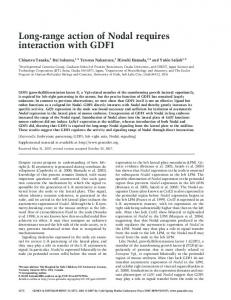
In this section we will present the main parameters for the geometrical setup and their optimization using simulated data. MC simulations were obtained by performing the variance minimization for the relative angle with respect to the beam axis and for the relative position of the tracking device with respect to the phantom. Indeed, the shape of the vertex distribution in the fall-off region was directly related to the variance value. The variance was therefore a good estimator for the fall-off range resolution. Secondary particle yields will also be discussed in this section. All the simulations were performed with a carbon ion beam at a fixed energy of 297.8 MeV/u.

5000

σ:

b)

12.4 ± 0.2 mm

Tail: 13.8 ± 0.1 %

4000

Position

50 40 30 20 5

10

15

dM

3000

20

25

30

35

40 Angle θ (o)

2000

1000

−0100 −80

−60

−40

−20

0

20

40

60

80

100

zrec-ztrue (mm)

pte

Figure 2. (a) Variance Vσ as a function of the angle (θ) between the tracker system and beam axis (red square) and variance VRM S as function of the distance between the first tracker plane and the phantom center (black circle). (b) Residual distance between simulated (true) and reconstructed (rec) longitudinal vertices position for the tracker placed at 10° with respect to the beam direction and at 20 cm from the phantom center. The red line is the fit result with a Gaussian function.

ce

3.1.1. Tracking device angle with respect to the beam axis: the tracker entrance was placed 20 cm from the phantom center (∼10 cm from the phantom edge). The variance was computed for different angles ranging from 5° to 40°. Variance Vσ was minimal when the tracking device placed at an angle of θ ∼10° with respect to the beam axis (see red squares in Figure 2a).

Ac

1 2 3 4 5 6 7 8 9 10 11 12 13 14 15 16 17 18 19 20 21 22 23 24 25 26 27 28 29 30 31 32 33 34 35 36 37 38 39 40 41 42 43 44 45 46 47 48 49 50 51 52 53 54 55 56 57 58 59 60


3.1.2. Tracking device longitudinal position with respect to the phantom center: since residual distributions tended to have a non Gaussian shape with decreasing distance, the variance VRM S was used. The variance was measured as a function of the tracker position with respect to the phantom center. The angle was set to the nominal value of 10°. The optimized value between the phantom center and the first plane of the tracker was around 20 cm (see black dots in Figure 2a).


10

pt


dM

an

us cri

3.1.3. Vertex resolution and particle yields: the distribution of the residual distance between simulated vertices, with the Bertini list, and reconstructed vertices (ztrue -zrec ), obtained for an θ = 10° angle and 20 cm distance to the tracker entrance is shown in Figure 2b. In this sample, the resolution evaluated by a Gaussian fit was σ = 12.4 ± 0.2 mm. As a comparison the resolution obtained with the BIC physics list was σ = 12.1 ± 0.2 mm. In addition the production rates of secondary particles were similar at the 2 % level for both physics lists (Bertini and BIC). The resolution degradation, when compared to the experiment with a thin target (Rescigno et al 2014), was mainly caused by the proton scattering in the phantom. The tail, as defined in (Rescigno et al 2014), was the relative proportion of events outside the fitted Gaussian function at ± 4σ, this was found to be less than 14%. Figure 3 presents the simulated angular distributions of secondary particle yields generated by nuclear reactions (Generated), scattered outside the phantom (Visible) and that hit at least three planes, of the tracking device (Reconstructible). Three planes were requested for the tracking to avoid the reconstruction of fake tracks that combine a real hit and a noisy hit. Only 30 % of the generated secondaries reached the phantom edge. The tracker covered a solid angle of 11.3 msr (0.09% of 4π). Only 4.8 % of the secondary particles emitted forward at θ = 10° impinged the CMOS detectors. ×10

Yield

3

140 120 100 80

pte

60

Generated Visible Reconstructible × 10

40 20

0 0

10

20

30

40

50

60

70

80 o Angle θ( )

ce

Figure 3. Secondary particle yield versus the emission angle (θ) with respect to the beam axis for the generated particles, the particles emerging from the phantom (visible) and the particles hitting the tracking device (reconstructible). A scaling factor of 10 was applied on the latter distribution. The limits (dashed lines) of the angular acceptance of the tracking device are also shown. The simulation was done with 106 carbon ions impinging on the PMMA phantom at an energy of 297.8 MeV/u.

Ac

1 2 3 4 5 6 7 8 9 10 11 12 13 14 15 16 17 18 19 20 21 22 23 24 25 26 27 28 29 30 31 32 33 34 35 36 37 38 39 40 41 42 43 44 45 46 47 48 49 50 51 52 53 54 55 56 57 58 59 60

Page 10 of 23

3.2. Alignment of the tracking device

A low intensity (< 104 particle/s) run was performed with the tracking device centered on the beam axis (θ = 0°), without the phantom, to reconstruct only the straight tracks. The tracker entrance was placed at 20 cm from the phantom center. The resultant

Page 11 of 23

11

pt


us cri

resolution of the residual distribution, was defined as the distance between the cluster positions and the reconstructed track line (Topi et al 2016). The minimization of the residual distributions led to a resolution better than 3 µm with the proportion of events outside the Gaussian shape being less than 7 %. The alignment parameters obtained for the eight CMOS sensors were used for all subsequent runs at an angle of θ = 10°. 3.3. Carbon ion monitoring and associated uncertainties

-1

Number of tracks (50ms )

pte

dM

an

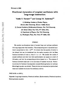
The number of carbon ions was measured with the tracking device. Indeed the number of reconstructed tracks was directly proportional to the number of the carbon ions impinging the target. Figure 4 shows the number of reconstructed tracks in a typical spill delivered by the synchrotron. The tracker device was situated 20 cm from the phantom center and at an angle of θ = 10°. The limits of the spill were computed using a threshold algorithm. The particle spill duration was 4.77 ± 0.05 s. To take into account the intra-spill variation, a linear fit was applied to the distribution. The residual in-spill variations relating to the fitted line were less than 5 %. The results of the fit were used when computing the number of impinging carbons for each given spill. The variation of the particle number between spills was around 7 %. The stability of the beam intensity between runs was measured with a beam hodoscope. The variation was about 8 %. The average value of the beam intensity at the extraction point was (4.5 ± 0.4)×106 carbon ions per second while the error due to pileup events in the hodoscope was less than 10 %. Thus the total uncertainty of the carbon ion was 15 %. Given the number of incident carbon ions, the yield of secondary particles per incident carbon ion was computed. For example , for run L01 (energy of 240.6 MeV/u), the resultant yield was (7.6 ± 0.5stat ± 1.1syst )×10−4 msr−1 per incident carbon ion.

3000 2500 2000 1500

ce

Ac

1 2 3 4 5 6 7 8 9 10 11 12 13 14 15 16 17 18 19 20 21 22 23 24 25 26 27 28 29 30 31 32 33 34 35 36 37 38 39 40 41 42 43 44 45 46 47 48 49 50 51 52 53 54 55 56 57 58 59 60


1000 500 0

26

28

30

32

34

36

38

40

Time (s)

Figure 4. Number of reconstructed tracks, with a 50 ms binning, for two consecutive spills. The results were obtained with data from run H05 at 297.8 MeV/u on the homogenous PMMA phantom. The vertical solid lines represent the computed limits of the spill. Linear fits (red) are also plotted, taking into account of the in-spill variation of the beam.


12

pt

Study for online range monitoring with the Interaction Vertex Imaging method 3.4. The IVI sensitivity study

us cri

First, to test the robustness of the method, the p-values were computed for different bin sizes of the vertex distributions: Sbin = 1 mm, 200 µm, 100 µm and 25 µm. The p-values were calculated for a displacement of ∆BP = 3.4 mm. For each bin size, the ˜12C was computed. The variation of parameter N ˜12C as a function of the bin value of N size was less than 0.3×106 carbon ions. A bin size of 100 µm was arbitrarily chosen, while the error related to the bin size was taken into account for the minimum number ˜12C . of carbon ions N

an

3.4.1. χ2 test for HE and LE runs: Table 2 summarizes the run number along with the corresponding BP position of the carbon ions for the HE and LE runs. For example, the vertex distributions corresponding to ∆BP = 3.4 mm were analyzed with their corresponding BP distributions (Figure 5a and Figure 5b). The distributions were obtained from data analysis with ∼107 incident carbon ions. The χ2 test was applied to the cumulative vertex distributions.

Run

dM

Table 2. Position of the Bragg Peak for HE and LE data. The third column corresponds to the difference in range (∆BP) while taking runs H05 and L05 as the respective reference. The last column represents for the minimum number of carbon ˜12C to disentangle the two vertex distributions. The corresponding errors also ions N include the 15 % uncertainties and 0.3×106 variations in the number of carbon ions. Bragg Peak (mm)

∆BP (mm)

˜12C (106 ) N

HE runs

140.31 141.11 142.06 142.87 143.74

± ± ± ± ±

0.01 0.01 0.01 0.01 0.01

pte

H01 H02 H03 H04 H05

3.43 2.63 1.68 0.87

± ± ± ± -

0.02 0.02 0.02 0.02

2.6 ± 0.7 4.2 ± 0.9 7.3 ± 1.4 > 10

± ± ± ± -

0.02 0.02 0.02 0.02

2.2 ± 0.8 4.5 ± 1.0 8.0 ± 1.7 > 10

LE runs

ce

L01 L02 L03 L04 L05

100.60 101.45 102.31 103.16 104.03

± ± ± ± ±

0.01 0.01 0.01 0.01 0.01

3.43 2.48 1.72 0.87

Probability p-values were computed for the HE and LE runs (Figure 5c and ˜12C are reported in Table 2. For example Figure 5d). The extracted values of N ˜12C corresponded to for ∆BP = 1.7 mm, the minimum number of carbon ions N 6 6 (7.3 ± 1.4)×10 and (8.0 ± 1.7)×10 for HE runs and LE runs respectively. In addition, even when the number of carbon ions exceeded 1.5×107 , it was not possible to separate the vertex distributions corresponding to ∆BP ' 0.9 mm. For each decreasing step ˜12C was observed. of 1 mm in ∆BP, an enhancement factor of approximately 1.5 in N

Ac

1 2 3 4 5 6 7 8 9 10 11 12 13 14 15 16 17 18 19 20 21 22 23 24 25 26 27 28 29 30 31 32 33 34 35 36 37 38 39 40 41 42 43 44 45 46 47 48 49 50 51 52 53 54 55 56 57 58 59 60

Page 12 of 23

3.4mm

Run H01

1200

250

1000

200

800

150

1000

Run L05

300

Run L01

3.4mm

800

250

us cri

Run H05

VertexZ (mm-1)

1400

b)

dE/dx (keV/mm)

VertexZ (mm-1)

a) 300

13

pt


200

600

100 400 50

20

40

60

80

100

120

140 160 Position (mm)

0

0

c)

1 0.9

HE Exp: ∆ BP = 0.9 ∆ BP = 1.7 ∆ BP = 2.6 ∆ BP = 3.4

20

40

60

0.7 0.6 0.5

80

100

120

0.9

50


1

0.7

0.6 0.5

0.4

0.4

0.3

0.3 0.2

0.1 2

4

dM

0.2

6 8 10 Number of incident ions (millions)

0.1 0

2

4


pte

Figure 5. (a) Longitudinal vertex distributions for run H05 (taken as reference) at an energy of 297.8 MeV/u and run H01 at an energy of 293.5 MeV/u. (b) Longitudinal vertex distributions for run L05 (taken as reference) at an energy of 245.4 MeV/u and run L01 at an energy of 240.6 MeV/u. Corresponding BP distributions are also plotted. These distributions were obtained with 107 incident carbon ions. (c) p-value of the χ2 test, performed using HE data, as a function of the number of carbon ions for ∆BP = 0.9 (black dot), 1.7 (red square), 2.6 (blue up triangle) and 3.4 (green down triangle) mm. The limits at p-value = 0.05 (dotted line) are also plotted. (d) p-value of the χ2 test, performed using LE data, as function of the number of carbon ions for ∆BP =0.9 (black dot), 1.7 (red square), 2.5 (blue up triangle) and 3.4 (green down triangle) mm. The limits at p-value = 0.05 (dotted line) are also plotted.

ce

The same trend was seen for LE and HE runs with regard to the minimum number of impinging carbon ions necessary to separate two vertex distributions. 3.4.2. χ2 test for bone and air insert position runs: The χ2 test was performed on data taken for Config2b and Config2a, i.e., bone and air insert position runs, respectively. Figure 6a shows the statistical significance (p-value) of the vertex distributions regarding the number of impinging carbon ions for the bone insert position runs. The ˜12C corresponded to (3.2 ± 0.8)×106 , (3.9 ± 0.9)×106 , minimum number of carbon ions N (1.4 ± 0.5)×106 and (2.6 ± 0.7)×106 for position 1 to 4, respectively. The uncertainties included statistical and systematic errors. Only when the insert was placed at the end

0

d)

LE Exp: ∆ BP = 0.9 ∆ BP = 1.7 ∆ BP = 2.5 ∆ BP = 3.4

0.8

an

0.8

p-value

p-value

0

100

200

200

0

150

400

600

Ac

1 2 3 4 5 6 7 8 9 10 11 12 13 14 15 16 17 18 19 20 21 22 23 24 25 26 27 28 29 30 31 32 33 34 35 36 37 38 39 40 41 42 43 44 45 46 47 48 49 50 51 52 53 54 55 56 57 58 59 60


dE/dx (keV/mm)

Page 13 of 23


14

pt


of the phantom at 120 mm from the phantom entrance (position 3), the method showed a slightly more pronounced sensitivity. It needed around a factor 2 less statistics for ˜12C this position compared to the other ones. For positions 1, 2 and 4, the values of N

χ2/NdF

0.35 Bone Insert: 1 2 3 4

0.3 0.25 0.2

30 25

b)

Air Insert: 1 2 3 4

20

0.15

15

0.1

10

0.05

5

1

2

3

4 5 6 7 8 Number of incident ions (millions)

dM

00

35

an

p-value

a)

us cri

overlapped within the error bars. As a results, no conclusion could be made concerning the sensitivity for those bone insert positions. For the air insert positions runs, the χ2 /NdF values versus the number of carbon ions are presented in Figure 6b. The same trend was observed as for the bone inserts, in particular, the sensitivity was greater when the insert was placed at position 3.

2

4


pte

Figure 6. (a) p-value of the χ2 test, performed on data with Config2b, versus the number of carbon ions for different insert positions. (b) The χ2 /NdF values were computed for data with Config2a, versus the number of carbon ions for different insert positions. The red square symbol stands for position 1, the blue up triangle symbol stands for position 2, the green down triangle symbol stands for position 3 and the black dot symbol stands for position 4.

ce

3.4.3. χ2 test for bone and air insert runs: Table 3 summarizes the bone and air insert run numbers and energy with the corresponding BP position for Config3b and Config3a, ˜12C are also reported in this table. respectively. The values of N The sensitivity of the method was less pronounced compared to the homogenous phantom data. The two vertex distributions started to differentiate, when ∆BP ˜12C = (5.3 ± 1.1)×106 and ∼ 3.3 mm, for a number of impinging carbon ions N ˜12C = (5.0 ± 1.7)×106 for bone and air data respectively. Compared to LE and N HE runs, this corresponded roughly to a factor 2 in the carbon ion number. Large ˜12C values were associated to a flat slope of the p-values near the 5 % error bars for N ˜12C > 107 and N ˜12C > (4.5 ± 1.2)×106 were needed to separate line. In addition, N the two vertex distributions for ∆BP ∼ 2.5 mm for bone and air inserts respectively (see Table 3). The sensitivity of the BP displacement was less pronounced for the bone insert (position 2) data compared to the air insert (position 3) data, as position 3 was ˜12C for the air data had the same more favorable in terms of sensitivity. Furthermore, N value within the error bars for a BP displacement of ∆BP = 2.6 or 3.4 mm.

Ac

1 2 3 4 5 6 7 8 9 10 11 12 13 14 15 16 17 18 19 20 21 22 23 24 25 26 27 28 29 30 31 32 33 34 35 36 37 38 39 40 41 42 43 44 45 46 47 48 49 50 51 52 53 54 55 56 57 58 59 60

Page 14 of 23

Page 15 of 23

15

pt


Run

Bragg Peak (mm)

∆BP (mm)

Bone insert runs (Config3b) B01 B02 B04 B05

99.52 ± 0.01 100.32 ± 0.01 102.00 ± 0.01 102.80 ± 0.01

3.28 ± 0.02 2.48 ± 0.02 0.80 ± 0.02 -

Air insert runs (Config3a)

3.5. Inflection points

± ± ± ± ±

0.01 0.01 0.01 0.01 0.01

3.39 2.59 1.70 0.88

± ± ± ± -

0.02 0.02 0.02 0.02

5.3 ± 1.1 -

5.0 ± 1.7 4.5 ± 1.2 -

an

140.36 141.16 142.05 142.87 143.75

˜12C (106 ) N

dM

A01 A02 A03 A04 A05

us cri

Table 3. BP position for the bone and air insert runs. The third column corresponds to the difference in range (∆BP) taking runs B05 and A05 as references, respectively. ˜12C needed to Column four represents for the minimum number of carbon ions N disentangle the two vertex distributions. The corresponding errors included also the 15 % and 0.3×106 variations in the number of carbon ions.

ce

pte

Inflection points were computed for the HE runs. Distributions were obtained for ∼2.4×107 incident carbon ions. The cumulative vertices were normalized. The results are shown in Figure 7a for the two extreme BP positions namely for runs H05 and H01 with the homogeneous phantom. Systematic error bars were computed to estimate the sensitivity to the range of the fit. The amplitude of the uncertainties was estimated around 0.3 mm. The inflection point position versus the BP position is shown in Figure 7b. The inflection points for the LE runs were computed using the second method. An example of the vertex distributions with the corresponding fit results, for the two outer BP positions (i.e., runs L05 and L01) is shown in Figure 7c. As with HE runs, the results were very sensitive to the range of the fits. Hence systematic errors were evaluated by changing the fitting range, with the uncertainties being around 0.3 mm. The correlation between the positions of the inflection point position and the corresponding BP position is shown in Figure 7d. By computing the inverse function, the relation between the inflection points and the BP position could be established for the HE and LE runs. The deduced BP position (BPinf l ) as function of the inflection point (IP) could be written as follows: √ BPinf l = A × IP + d + B (2)

Ac

1 2 3 4 5 6 7 8 9 10 11 12 13 14 15 16 17 18 19 20 21 22 23 24 25 26 27 28 29 30 31 32 33 34 35 36 37 38 39 40 41 42 43 44 45 46 47 48 49 50 51 52 53 54 55 56 57 58 59 60


1

where parameters A, d and B are 2.9 mm 2 , -141.2 mm and 139.2 mm for the HE 1 runs and 2.3 mm 2 , -90.9 mm and 99.4 mm for the LE runs, respectively. ˜12C values For the HE and LE runs the inflection points were computed from the N


0.6

0.85

144 143.5 143

us cri

BP position: 145.8 mm 142.4 mm

0.8

b)

Inflection Point (mm)

Normalized counts

a) 1

16

pt


142.5 0.8

0.4

142

0.75 0.7 120

0.2

125

130

141.5

135

141

0

80

100

120

140

140

160

BP position: 104.0 mm 100.6 mm

1400

141

141.5

142

142.5

143

143.5

144

d)

95.5 95

94.5 94

an

1200

Inflection Point (mm)

VertexZ (mm-1)

c) 1600

140.5

Bragg Peak (mm)

Position (mm)

1000

93.5 93

800

92.5

600

92

400 200 0

0

20

40

60

80

dM

91.5

100

120


91 100.5

101

101.5

102

102.5

103

103.5

pte

(see Table 2) and the associated BP position (BPinf l ) deduced from Equation (2). The results are summarized in Table 4. The BP position for each given couple was separated at a 1σ level, except for ∆BP = 0.9 mm. The accuracy of the BP positions ranged from 0.5 to 1 mm for the HE runs. In the case of LE runs, the BPinf l positions for each given ∆BP were less separated than for the HE runs. Indeed, the accuracy of the BP positions ranged from 1 to 2 mm. The BPinf l position computed from the inflection points and the theoretical BP position were equal within the error bars regardless of whether the run was HE or LE. In the same way the inflection points and the associated BPinf l positions were ˜12C was computed for bone and air insert runs. The accuracy of the BP positions, for N above 1mm and 2 mm for the bone and air insert runs respectively (results not shown).

ce

104

Bragg Peak (mm)

Figure 7. (a) Cumulative vertex distributions for two HE runs (i.e., run H05 and H01) with the corresponding sigmoid fits. A close-up of these distributions, for range of 120 to 136 mm, is depicted in the inset. (b) Inflection point position versus the BP position for HE runs. The resulting points were fitted with a second order polynomial. The error bars reflect only the statistical uncertainties. (c) Vertex distributions for the two LE runs (i.e., run L05 and L01) with the corresponding linear fits. (d) Inflection point position versus the BP position for the LE runs. The resulting points were fitted with a second order polynomial. The error bars reflect only the statistical uncertainties. The distributions were obtained with ∼2.4×107 incident carbon ions.

Ac

1 2 3 4 5 6 7 8 9 10 11 12 13 14 15 16 17 18 19 20 21 22 23 24 25 26 27 28 29 30 31 32 33 34 35 36 37 38 39 40 41 42 43 44 45 46 47 48 49 50 51 52 53 54 55 56 57 58 59 60

Page 16 of 23

Page 17 of 23

17

pt


HE runs BPinf l (mm)

Bragg Peak (mm)

H01 H05

140.5 ± 0.7 144.1 ± 1.0

140.31 ± 0.01 143.74 ± 0.01

H02 H05

141.9 ± 0.7 144.0 ± 0.7

141.11 ± 0.01 143.74 ± 0.01

H03 H05

142.1 ± 0.4 144.0 ± 0.5

142.06 ± 0.01 143.74 ± 0.01

H04 H05

143.1 ± 0.5 143.9 ± 0.5

142.87 ± 0.01 143.74 ± 0.01

∆BP (mm)

˜12C (106 ) N

3.43 ± 0.02

2.6

2.63 ± 0.02

4.2

1.68 ± 0.02

7.3

an

Run

us cri

Table 4. Position of the extrapolated BP position (BPinf l ) from the inflection point for HE and LE data. The third column is the theoretical BP position. The fourth column corresponds to the difference in range (∆BP) when taking runs H05 and L05 as references, respectively. The last column represents the minimum number of carbon ˜12C required to compute the inflection points. ions N

0.87 ± 0.02

10

LE runs

99.4 ± 1.5 103.2 ± 2.0

100.60 ± 0.01 104.03 ± 0.01

3.43 ± 0.02

2.2

L02 L05

101.2 ± 1.0 103.7 ± 1.5

101.45 ± 0.01 104.03 ± 0.01

2.48 ± 0.02

4.5

L03 L05

102.6 ± 1.0 103.9 ± 1.0

102.31 ± 0.01 104.03 ± 0.01

1.72 ± 0.02

8.0

L04 L05

103.3 ± 1.0 103.9 ± 1.0

103.16 ± 0.01 104.03 ± 0.01

0.87 ± 0.02

10

pte

dM

L01 L05

4. Discussion

ce

A method based on the χ2 test was used to study the sensitivity of the IVI technique as function of the number of impinging carbon ions. To assess the minimum number of carbon ions needed to disentangle vertex distributions for a given displacement in BP, an experiment was conducted at HIT center. 4.1. Geometry setup

The yield of secondary particle measured, for run L01, was (7.6 ± 0.5stat ± 1.1syst )×10−4 msr−1 per incident carbon ion with an energy of 240.6 MeV/u (see Section 3.3). A similar setup with a 127.8 mm water target was used irradiated by a carbon ion beam at 200 MeV/u energy (Gunzert-Marx et al 2008). A telescope was placed behind the target to identify the secondary particles. The proton production for an azimuthal angle of 10° was (4.2 ± 0.1)×10−4 msr−1 per incident carbon ion. The difference between the two production rates originated from the higher energy and target density (water vs

Ac

1 2 3 4 5 6 7 8 9 10 11 12 13 14 15 16 17 18 19 20 21 22 23 24 25 26 27 28 29 30 31 32 33 34 35 36 37 38 39 40 41 42 43 44 45 46 47 48 49 50 51 52 53 54 55 56 57 58 59 60



18

pt


pte

dM

an

us cri

PMMA) used in this study In our work, we demonstrated that the larger angles (θ > 15°) and closer positions (< 20 cm) of the tracking device, with respect to the phantom (see Figure 2a), diminished the sensitivity of the fall-off in vertex distributions. Indeed an azimuthal angle of θ = 10° minimized the variance distribution. These position and angle values exhibited the best compromise between a good resolution σ on the single longitudinal vertex distribution and a high number of vertices. The angular distribution of fragments are peaked in the beam direction due to nuclear reaction kinematics (Matsufuji et al 2005). Hence, the lower the angle, the higher the number of reconstructed vertices, although the resolution in vertex position was lower. Indeed, the variance Vσ is twice worse for an angle of θ = 30° compared to θ = 10° (see red squares in Figure 2a). The statistical loss at θ = 30° is not compensated by the improved resolution on a single vertex. When the tracking device was placed as close as possible to the phantom (typically, a few centimeters from its end), a severe loss in resolution with a non-Gaussian shape in the distribution was observed (see black dot in Figure 2a). For a tracker distance of 11 cm from the phantom center, the RMS of the residual distribution was 1.8 times higher compared to the optimal tracker position at 20 cm. This difference was ascribed to secondary vertices due to protons emitted in the second step of the processes (i.e., rescattering, fragmentation of primary fragments, etc.), which were mainly produced in the BP region. The particles, generated from such processes, had shifted vertices. Therefore, by placing the tracking device closer to the phantom, the detection of secondary vertices was favored, but the vertex resolution was reduced. On the contrary when the tracker was placed at greater distance (> 20 cm), the number of reconstructed vertices decreased while the resolution remained constant compared to the nominal distance. The optimal resolution is presented in Figure 2b. The tail in the distribution was due to proton scattering inside the phantom medium. The asymmetry in the tail was ascribed to the different proton path lengths in the phantom. Indeed, protons produced at the beginning of the target are more affected by scattering effects and as a result, the reconstructed vertex has a lower resolution. 4.2. Inflection point determination

ce

Regardless of the method used, the quadratic behavior of the inflection point as function of the BP was observed on a few millimeters range (see Figure 7b and Figure 7d). A non-linear effect was already reported by (Henriquet et al 2012) for ion ranges greater than 150 mm. Since only few inflection points were measured for smaller ion ranges, we cannot conclude whether or not some quadratic effects are present. For (Gwosch et al 2013), the error bars corresponding to the inflection points for small ∆BP were too large to draw any conclusion about non-linear effects. In our study, the relation between the BP positon and the inflection point exhibited a non-linear correlation for small ∆BP < 4 mm. The vertex distributions were distinguishable for a number of carbon ions greater

Ac

1 2 3 4 5 6 7 8 9 10 11 12 13 14 15 16 17 18 19 20 21 22 23 24 25 26 27 28 29 30 31 32 33 34 35 36 37 38 39 40 41 42 43 44 45 46 47 48 49 50 51 52 53 54 55 56 57 58 59 60

Page 18 of 23

Page 19 of 23

19

pt


dM

an

us cri

˜12C , based on the χ2 test (see Table 4). Although the distributions differed at than N the 2σ level, the corresponding inflection points were distinct below this level. The distance between the BPinf l positions and the reference runs was smaller for the LE runs compared to the HE runs. This implied a lower sensitivity of the IVI method for LE carbon beam compared to a HE beam. The accuracy of BPinf l positions in the presence of an insert exceeded 1 mm (see the end of Section 3.5). In addition, more reconstructed vertices were needed in order to achieve this accuracy compared to a homogenous phantom setup for a given ∆BP (for some examples see Table 3 and Table 2 for ∆BP ∼ 3.4 mm). The monitoring of the carbon ion range for an active beam delivery should provide information about any BP displacement for each raster position. Typically for a treatment fraction, ∼109 carbon ions (corresponding to 1 Gy) are used to irradiate a tumor measuring 120 cm3 . With around 104 raster scan positions, the number of impinging carbon ions per raster position ranges from 104 to 106 (value at the distal edge) (Krämer et al 2000). In (Henriquet et al 2012), the resolution of the BP versus the number of incident carbon ions was simulated while assuming the perfect response of the detector (no noise, no fake tracks or no residual misalignment of the tracking device, etc.). The authors shown a variation in the resolution of the inflection point with the square root of the number of incident carbon ions (Section 3.5). Using a quadratic extrapolation (see Table 4), the accuracy of the BP position can be deduced under clinical conditions (106 carbon ions for a single raster point for the distal plane) with the optimized setup using a homogeneous PMMA phantom. The obtained value would thus be around 4 to 5 mm. The situation deteriorates when inserts of bone or air are present.

pte

4.3. The IVI sensitivity study

ce

For a BP displacement of ∆BP < 1 mm, the corresponding vertex distributions obtained with the homogenous phantom (i.e., HE and LE data) could not be distinguishable at the 2σ level, even when the number of impinging carbon ions exceeded 106 (see Table 2). This was also reported with other modalities such as prompt-γ (Priegnitz et al 2015) and as in-beam PET systems (Piliero et al 2015). Typically for ∆BP < 2 mm, the number of incident carbon ions must exceed 7×106 . When inserts (bone or air in our case) were present in the phantom the vertex distributions were less distinguishable compared to homogenous phantoms. Indeed, the error in the reconstructed vertex increased as the proton crossed materials of different densities, leading to higher p-values. The IVI method was less sensitive if the beam intercepted heterogeneities. Indeed, for the bone insert, the separation of two vertex distributions was only possible for ∆BP > 3.3 mm with a corresponding number of ˜12C > 5×106 (see Table 3), while for the homogeneous PMMA target the carbon ions N vertices distributions were distinguishable for ∆BP < 2 mm. For prompt-γ monitoring with the proton beam impinging on a heterogeneous phantom, range shifts were detected

Ac

1 2 3 4 5 6 7 8 9 10 11 12 13 14 15 16 17 18 19 20 21 22 23 24 25 26 27 28 29 30 31 32 33 34 35 36 37 38 39 40 41 42 43 44 45 46 47 48 49 50 51 52 53 54 55 56 57 58 59 60



20

pt


dM

an

us cri

with an accuracy of 2-5 mm, depending on the proton statistics (Hueso-González et al 2015). Similar results, using a clinical proton beam, were obtained with in-room PET where the range shifts were measured with uncertainties less than 5 mm (Min et al 2012). These detected range shifts were comparable with the values of our study. For a heterogeneous phantom, around twice as many incident carbon ions were needed to separate two vertex distributions for a given ∆BP compared to a homogeneous phantom. Therefore, whenever anatomical changes occur between treatment planning and irradiation (e.g., nasal congestion), the IVI method will be less accurate for online control. When the carbon ions passed through an inhomogeneity the sensitivity was slightly more pronounced when the insert was located at the end of the phantom, near the BP position (see Figure 6a and Figure 6b). In this case, the insert was located closer to the detector, and the resolution of the reconstructed vertex was better given the shorter extrapolated distance. For a more upstream insert position the proton path in the medium was longer, and as a result, the reconstructed interaction vertex was more blurred. Therefore, the sensitivity of the method depended on the relative position of the detector with respect to the inhomogeneity. In our case, the insert had a diameter of 28 mm and completely intercepted the beam (FWHM = 4.2 mm). Sensitivity would be lower when only part of the beam impinges on the insert. 4.4. Full ring detector considerations

ce

pte

To increase the number of reconstructed vertices, the acceptance of our tracking device could be improved. Since the distribution of the secondary particles (see Figure 3) was peaked at forward angles, one way was to improve the detector acceptance would be to use a full-ring detector. In this case a factor of 21 in the number of reconstructed vertices could be obtained, leading to a reduction in statistical fluctuations by a factor 4.6. As an example, according to Table 4, for a displacement of ∆BP = 1.7 mm, with runs H03 and ˜12C = (1.6 ± 0.2)×106 . H05, the minimum number of carbon ions can be reduced to N Taking into account the 4.6 reduction factor for runs H02 and H05, the number ˜12C ∼ 106 while the corresponding BP accuracy was 0.7 mm (see of carbon ions was N Table 4). By adding the systematic errors coming from the fitting range, the final accuracy of the BP position was around 1 mm. For the LE runs, (see runs L02 and L05 in Table 4), the accuracy of the BP position with 106 carbon ions, was about 1.5 mm, including the systematic errors. In both HE and LE runs, with a full-ring tracking device, the accuracy of the BP position was reduced to 1 and 1.5 mm under clinical conditions (i.e., 106 incident carbon ions). The same conclusions were made by (Henriquet et al 2012) who described a millimeter BP resolution for 106 incident carbon ions and about 1.5 mm for 2×105 incident carbon ions. Nevertheless, the results were obtained with lower statistics with a factor 1.5 compared to the one obtained with a full-ring detector. This difference was mainly due to the overestimation of the secondary particle production rate in simulations compared to real data (see Section 2.2).

Ac

1 2 3 4 5 6 7 8 9 10 11 12 13 14 15 16 17 18 19 20 21 22 23 24 25 26 27 28 29 30 31 32 33 34 35 36 37 38 39 40 41 42 43 44 45 46 47 48 49 50 51 52 53 54 55 56 57 58 59 60

Page 20 of 23

Page 21 of 23

21

pt


dM

5. Summary and conclusion

an

us cri

Furthermore, increasing the detector size generates additional uncertainties. The alignment of the different modules of such a tracking device has to be done accurately to minimize the impact of the vertex reconstruction. The referential of the detector has to perfectly match either the patient or the treatment room referential. We should keep in mind that constraints exist in the clinical treatment room. The detector and the associated services should be kept as small as possible to avoid any conflict with the beam apparatus and to preserve the comfort of the patient. In addition the IVI technique relies on the comparison between the vertex profiles computed using the treatment planning system and the measured ones. Therefore, it is necessary to have a good knowledge of all underlying processes (i.e., fragmentation cross-section values). Previous works (Napoli et al 2012, Dudouet et al 2003) have already pointed the difficulties for models to properly reproduce the production yield of secondary particles especially at low azimuthal angles (< 5°). A detailed study, taking into account all the sources of uncertainties and the clinical constraints should therefore be undertaken to really assess the millimetric accuracy of the BP position using the IVI method.

ce

pte

A statistical study was undertaken to assess the IVI sensitivity of experimental data collected at the HIT center. Our IVI tracking device based on a CMOS pixel sensor technology was used to measure interaction vertices during phantom irradiation with carbon ion beams. A phantom with and without inserts of different materials was used. Our reduced-size tracker device with a 11.3 msr solid angle coverage, could typically achieve 3 mm ∆BP sensitivity with ∼3.5×106 incident ions in a homogenous phantom. Higher statistics (factor 2) were needed in order to obtain the same sensitivity when heterogeneities were inserted close to the end of the ion range. Nevertheless, an extrapolation of a full-ring detector in clinical conditions may result in a accuracy of the BP position about 1-2 mm. This, however, requires a complete study including all statistical and systematical errors to assess a millimetric resolution using an IVI technique under clinical conditions. With the IVI technique, it will be possible to consequently reduce the margins to assure the target coverage. Acknowledgments

The study conducted at HIT was supported by the Plan Cancer 2011 in the framework of the INCa-QAPIVI project. The authors wish to thank the HIT for the beam time and technical support. Beam time at the HIT was granted by the European FP7 project ULICE (grant agreement no. 228436). This work was also supported by the RhôneAlpes Region. It is now undertaken in the framework of the ANR France Hadron (ANR-11-INBS-0007) and Nuclear Physics Institute of Lyon as part of the LABEX PRIMES (ANR-11-LABX-0063).

Ac

1 2 3 4 5 6 7 8 9 10 11 12 13 14 15 16 17 18 19 20 21 22 23 24 25 26 27 28 29 30 31 32 33 34 35 36 37 38 39 40 41 42 43 44 45 46 47 48 49 50 51 52 53 54 55 56 57 58 59 60



22

pt

Study for online range monitoring with the Interaction Vertex Imaging method References

ce

pte

dM

an

us cri

Agostinelli S, Allison J and Amako K 2003 Geant4a simulation toolkit Nucl. Instrum. Methods A 506, 250–303 Amaldi U, Hajdas W, Iliescu S, Malakhov N, Samarati J, Sauli F and Watts D 2010 Advanced Quality Assurance for CNAO Nucl. Instrum. Methods A 617, 248–249 Brun R and Rademakers F 1997 ROOT An object oriented data analysis framework Nucl. Instrum. Methods A 389, 81–86 Doane D P 1976 Aesthetic frequency classification The American Statistician 30, 181–183 Dudouet J, Cussol D, Durand D and Labalme M 2014 Benchmarking geant4 nuclear models for hadron therapy with 95 MeV/nucleon carbon ions Phys. Rev. C 89, 054616. Enghardt W, Crespo P, Fiedler F, Hinz R, Parodi K, Pawelke J and Pönisch F 2004 Charged hadron tumour therapy monitoring by means of PET Nucl. Instrum. Methods A 525, 284–288 Fiedler F et al 2008 In-beam PET measurements of biological half-lives of 12C irradiation induced beta+-activity. Acta Oncol. 47(6), 1077–86 Folger G, Ivanchenko, V and Wellisch, J 2004 The Binary Cascade - Nucleon nuclear reactions Eur. Phys. J. A 21 (3), 407-417 Gagunashvili N 2005 χ2 test for comparison of weighted and unweighted histograms. Statistical Problems in Particle Physics, Astrophysics and Cosmology Proc. of PHYSTAT05 , 12–15 Gianoli C et al 2017 First clinical investigation of a 4D maximum likelihood reconstruction for 4D PET-based treatment verification in ion beam therapy Radiotherapy & oncology 123(3), 339345 Gunzert-Marx K, Iwase H, Schardt D and Simon R S 2008 Secondary beam fragments produced by 200 MeV/u 12C ions in water and their dose contributions in carbon ion radiotherapy New J. Phys. 10, 075003 Gwosch K, Hartmann B, Jakubek J, Granja C, Soukup P, Jäkel O and Martiˇs´ıková M 2013 Noninvasive monitoring of therapeutic carbon ion beams in a homogeneous phantom by tracking of secondary ions Phys. Med. Biol. 58, 3755–73 Helmbrecht S et al 2013 Analysis of metabolic washout of positron emitters produced during carbon ion head and neck radiotherapy Med. Phys 40(9), 091918 Henriquet P et al 2012 Interaction vertex imaging (IVI) for carbon ion therapy monitoring: a feasibility study Phys. Med. Biol. 57(14), 4655–69 Hu-Guo C et al 2010 First reticule size MAPS with digital output and integrated zero suppression for the EUDET-JRA1 beam telescope Nucl. Instrum. Methods A 623, 480–482 Hueso-Gonz´ alez F et al 2015 First test of the prompt gamma ray timing method with heterogeneous targets at a clinical proton therapy facility Phys. Med. Biol. 60, 6247–6272 Knopf A, Parodi K, Bortfeld T, Shih H A and Paganetti H 2009 Systematic analysis of biological and physical limitations of proton beam range verification with offline PET/CT scans Phys. Med. Biol. 54, 4477–4495 Koi T 2008 New native QMD code in Geant4 IEEE Nuclear Science Symposium Conf. Record Kr¨ amer M, J¨ akel O, Haberer T, Kraft G, Schardt D and Weber U 2000 Treatment planning for heavyion radiotherapy: physical beam model and dose optimization Phys. Med. Biol. 45, 3299317 Marafini M et al The INSIDE Project: Innovative Solutions for In-Beam Dosimetry in Hadrontherapy Acta Phys. Pol. 127, 1465–1467 Matsufuji N et al 2005 Spatial fragment distribution from a therapeutic pencil-like carbon beam in water Phys. Med. Biol. 50, 3393–3403 McGowan S G, Burnet N G and Lomax A J 2013 Treatment planning optimisation in proton therapy British Journal of Radiology 86(1021) Min C H, Kim C H, Youn M Y and Kim J W 2006 Prompt Gamma Measurements for Locating the Dose Falloff Region in the Proton Therapy Appl. Phys. Lett. 89 Min C H et al 2012 Clinical Application of In-Room Positron Emission Tomography for In Vivo

Ac

1 2 3 4 5 6 7 8 9 10 11 12 13 14 15 16 17 18 19 20 21 22 23 24 25 26 27 28 29 30 31 32 33 34 35 36 37 38 39 40 41 42 43 44 45 46 47 48 49 50 51 52 53 54 55 56 57 58 59 60

Page 22 of 23

Page 23 of 23

23

pt


ce

pte

dM

an

us cri

Treatment Monitoring in Proton Radiation Therapy Int. J. Radiat. Oncol. Biol. Phys. 86(1), 182–189 Moteabbed M, Espa˜ na S and Paganetti H 2011 Monte Carlo patient study on the comparison of prompt gamma and PET imaging for range verification in proton therapy Phys. Med. Biol. 56, 1063– 1082 De Napoli M et al 2012 Carbon fragmentation measurements and validation of the Geant4 nuclear reaction models for hadrontherapy Phys. Med. Biol. 57, 7651–7671 Paganetti H 2012 Range uncertainties in proton therapy and the role of Monte Carlo simulations Phys. Med. Biol. 57(11), R99–117 Parodi K, Bortfeld T, and Haberer T 2008 Comparison between in- beam and offline positron emission tomography imaging of proton and carbon ion therapeutic irradiation at synchrotron- and cyclotron-based facilities International journal of radiation oncology, biology, physics 71 945–56 Parodi K et al 2008 PET imaging for treatment verification of ion therapy: Implementation and experience at GSI Darmstadt and MGH Boston Nucl. Instrum. Methods A 591, 282–286 Piersanti L et al 2014 Measurement of charged particle yields from PMMA irradiated by a 220 MeV/u 12 C beam Phys. Med. Biol. 59(7), 1857–72 Piliero M A et al 2015 Performance of a fast acquisition system for in-beam PET monitoring tested with clinical proton beams Nucl. Instrum. Methods A 804, 163–166 Pleskac R et al 2012 The FIRST experiment at GSI Nucl. Instrum. Methods A 678, 130–138 Priegnitz M, Helmbrecht S, Janssens G, Perali I, Smeets J, Vander Stappen F, Sterpin E and Fiedler F 2015 Measurement of prompt gamma profiles in inhomogeneous targets with a knife-edge slit camera during proton irradiation Phys. Med. Biol. 60(12), 4849-71 Rescigno R et al 2014 Performance of the reconstruction algorithms of the FIRST experiment pixel sensors vertex detector Nucl. Instrum. Methods A 767, 34–40 Scott D W 1979 On optimal and data-based histograms Biometrika 66, 605–610 Schardt D, Elssser and Schulz-Ertner D 2010 Heavy-ion tumor therapy: Physical and radiobiological benefits Rev. Mod. Phys. 82, 383-426. Sturges H A 1926 The choice of a class interval Journal of the American Statistical Association 21(153), 65–66 Testa E et al 2009 Dose profile monitoring with carbon ions by means of prompt-gamma measurements Nucl. Instrum. Methods B 267, 993–996 Testa E et al 2008 Monitoring the Bragg peak location of 73MeV/u carbon ions by means of prompt γ-ray measurements Appl. Phys. Lett. 93 Testa M et al 2010 Real time monitoring of the Bragg-peak position in ion therapy by means of single photon detection Radiation and Environmental Biophysics 49, 337–343 Thomas S J 2006 Margins for treatment planning of proton therapy Phys. Med. Biol. 51, 1491-1501 Toppi M et al 2016 Measurement of fragmentation cross sections of C12 ions on a thin gold target with the FIRST apparatus Phys. Rev. C 93, 064601 Woodward W.A, Amos R.A 2016 TProton Radiation Biology Considerations for Radiation Oncologists Int J Radiat Oncol Biol Phys. 95(1), 5961 Wright D.H and Kelsey M.H 2015 The Geant4 Bertini Cascade Nucl. Instrum. Methods A 804, 175188

Ac

1 2 3 4 5 6 7 8 9 10 11 12 13 14 15 16 17 18 19 20 21 22 23 24 25 26 27 28 29 30 31 32 33 34 35 36 37 38 39 40 41 42 43 44 45 46 47 48 49 50 51 52 53 54 55 56 57 58 59 60


Study for online range monitoring with the Interaction ...

Study for online range monitoring with the Interaction ...

Suggest Documents

Nuclear response for the Skyrme effective interaction with zero-range ...

Fracture model with variable range of interaction

Breathers on lattices with long range interaction

Fracture model with variable range of interaction

Close range Photogrammetry for the Structural Monitoring of the Star ...

Scaling of dynamics with the range of interaction in short-range

Monitoring and Evaluation - InterAction

Monitoring and Evaluation - InterAction

Ontology Models for Interaction Design: Case Study of Online Support

Rotavirus VP8*: Phylogeny, Host Range, and Interaction with Histo ...

Long-range action of Nodal requires interaction with GDF1 - Genes ...

BCS-BEC crossover with a finite-range interaction

Fractional dynamics of coupled oscillators with long-range interaction

Spin exchange interaction with tunable range between graphene ...

User interaction with remote access to range-related ... - TU Chemnitz

Monitoring techniques for the study of deformations

Study of Interaction of Chitosan with Fluoride

Electrochemical Study of Doxorubicin Interaction with Different ...

Parametric study of the solar wind interaction with the Hermean ...

A Multiple Drug Interaction Study of Stavudine with Agents for ...

Spectroscopic study of the interaction between ... - Wiley Online Library

Ultrasonic Monitoring of the Interaction between ...

Online Map Games â playful interaction with

An advanced online monitoring approach to study the ...

Study for online range monitoring with the Interaction ...