Hindawi Shock and Vibration Volume 2018, Article ID 1043298, 13 pages https://doi.org/10.1155/2018/1043298
Research Article Study of Testing Method for Dynamic Initiation Toughness of Sandstone under Blasting Loading Dingjun Xiao ,1,2 Zheming Zhu ,1 Rong Hu,1 and Lin Lang1 1
MOE Key Laboratory of Deep Underground Science and Engineering, College of Architecture and Environment, Sichuan University, Chengdu 610065, China 2 Shock and Vibration of Engineering Materials and Structures Key Laboratory of Sichuan Province, Southwest University Science and Technology, Mianyang, Sichuan 621010, China Correspondence should be addressed to Zheming Zhu;
[email protected] Received 24 September 2018; Revised 15 November 2018; Accepted 25 November 2018; Published 24 December 2018 Academic Editor: Alvaro Cunha Copyright © 2018 Dingjun Xiao et al. This is an open access article distributed under the Creative Commons Attribution License, which permits unrestricted use, distribution, and reproduction in any medium, provided the original work is properly cited. In this paper, an internal central single-cracked disk (ICSCD) specimen was proposed for the study of dynamic fracture initiation toughness of sandstone under blasting loading. The ICSCD specimen had a diameter of 400 mm sandstone disc with a 60 mm long crack. Blasting tests were conducted by using the ICSCD specimens. The blasting strain-time curve was obtained from the radial strain gauges placed around the blast hole. The fracture initiation time was determined by circumferential strain gauges placed around the crack tip. The stress history on the blast hole of the sandstone specimen was then derived from measured strain curve through the Laplace transform. The numerical solutions were further obtained by the numerical inversion method. A numerical model was established using the finite element software ANSYS. The type I dynamic stress intensity factor curves of sandstone under blasting loading were derived by the mutual interaction integration method. The results showed that (1) the ICSCD specimen can be used to measure dynamic initiation fracture toughness of rocks; (2) the stress on the blast hole wall can be obtained by the Laplace numerical inversion method; (3) the dynamic initiation fracture toughness of the ICSCD sandstone specimen can be calculated by the experimental-numerical method with a maximum error of only 7%.
1. Introduction Drilling and blasting is one of the most common, economical, and efficient technologies, and it has been widely utilized in rock mass excavation and engineering construction applications. However, the use of such techniques in engineering practices has also raised considerable engineering stability and safety issues for researchers all over the world [1–3]. Understanding the dynamic fracturing behavior of rock as a heterogeneous material under blasting loading has important implications for both realizing more efficient rock breakage and preservation of rock masses. Therefore, exploring the behavior of rock under dynamic loading conditions has drawn special attention [4, 5]. In particular, how rocks break under blasting loading, the size distribution of the rock fragments, and the level of damage to the remaining rock body are some of the key issues explored in many research studies.
As natural materials, rocks contain large numbers of microcracks. These microcracks can affect the sizes of the fragments after blasting and, in certain cases, result in instability issues in rock engineering. The dynamic fracture toughness is an important rock parameter that measures its resistance to dynamic crack initialization and growth, as well as its ability to arrest cracks. Exploring the dynamic fracture toughness of rock samples allows researchers understand the characteristics of crack initialization, growth, and arrest, thus enabling them to predict and control the fracturing behavior of rocks. In summary, measuring the dynamic fracture toughness of rocks is the basis for investigating their dynamic fracturing behavior, which requires a strong theoretical background and advanced experimental techniques. A disc specimen and developed different configurations for loading the test sample were redesigned based on the Hopkinson pressure bar [6, 7]. Zhou et al. [8] and Zhang et al. [9] redesigned a disc specimen and developed different
2 configurations for loading the test sample based on the Hopkinson pressure bar. He further loaded the experimental measurement data onto commercial finite element software to perform extensive calculations and proposed a combined experimental-numerical approach to test the dynamic fracture toughness of rock samples. Zhou et al. [10] proposed an NSCB method to test the dynamic initiation fracture toughness of rock samples using the Hopkinson pressure bar as the loading platform. His method was further recommended by ISRM as a standard dynamic rock testing method. However, many achievements have been made in dynamic rock studies using the Hopkinson pressure bar as the loading platform. Blasting load is more complicated than the impacting load. First, the wave types are different. The impact-induced stress wave is one-dimensional wave, whereas the blast-induced stress wave can be a cylindrical, spherical, or plane wave. Second, the loading rates are different. The loading rate of blasts is generally larger than that of impacts. Both the explosive stress wave and explosive gases in the drilling and blasting processes affect rock fracture [11, 12]. Therefore, exploring the fracture toughness of rock samples under blasting loading is a more appropriate approach to resolving engineering blasting issues. Rocks are brittle material with natural cracks. Their inertia and size can often affect test results [13, 14]. The maximum allowable diameter of the Hopkinson pressure bar is usually around 100 mm, which imposes a severe limitation on the size of the rock specimen. It is generally more challenging to analyze the dynamic fracture behavior of rock specimens with smaller sizes. Therefore, design of testing platforms that allows the study of fracture toughness of large rock specimens is a necessary task, which can provide valuable information on rock blasting excavation engineering and stability analysis of rock mass after excavation. In this study, we designed and rationalized a test configuration for studying the dynamic fracture toughness under blasting loading by drilling and blasting in rocks. A new testing method was also proposed for obtaining the initiation fracture toughness of rocks. Using the proposed method, we obtained the dynamic initiation fracture toughness of the rock specimen under blasting loading conditions. Such methods can contribute to the enrichment of testing approaches for evaluating the dynamic fracture toughness of rocks. The flow chart of experimental numerical method is shown in Figure 1.
2. Design of Blasting Loading and Test Specimen Configurations 2.1. Blasting Loading Device. The use of high-pressure loading devices is a popular approach for studying the dynamic performance of materials at high strain rates. With increasing in-depth studies of the dynamic properties of materials, high-pressure loading techniques have been receiving more attention from researchers. Techniques such as dropping hammer, Hopkinson pressure bar, light gas gun, and explosive blasting [15, 16] have been widely used for studying the dynamic properties of materials. Compared to other dynamic loading methods, explosive blasting is a more
Shock and Vibration Strain measurement near the blast hole
Backcalculated pressure curve
Calculation of dynamic stress intensity factor Fracture initiation time measurement
Dynamic initiation fracture toughness
Figure 1: Flow chart of experimental numerical method.
advantageous approach for being simple, convenient, low cost, and free of size limitations. However, the explosive blasting method also entails complex loading mechanism and has poor repeatability and stability. Therefore, many researchers have developed alternative explosive blasting methods such as the explosive plane-wave generator and the explosive expansion ring [17] for analyzing the dynamic properties of materials under blasting loading conditions. In this study, the structure of an explosive loading device was designed from the engineering drilling and blasting perspective. An industrial detonating cord was used to generate stable and reliable blasting loads. The detonating cord was filled with 12 g of powder at every meter. The outer diameter and detonation velocity of the detonating cord were 5 mm and 6690 m/s, respectively. In order to minimize the radius of the explosive pack in the rock-pulverizing zone (3–7) r, and to strengthen the stress wave, the pulverizing zone was filled with water so that the detonating cord and the blasting wall were coupled by water, which enabled transmission of the explosive stress wave. In order to prevent early release of the explosive gases and to restrict the displacement in the Z direction for achieving a quasi-plane strain condition, the specimen was covered with a plate made from the same materials on both the top and bottom surfaces. The blasting holes were coupled with the platecovering by high-strength explosion-proof tubes for reducing the damage on the plate-covering from the detonating cord. The configuration of the loading device is shown in Figure 2. According to the literature, the testing specimen can be considered to be under plane stress if the strain of the specimen in the Z direction under dynamic loading is less than 1/5 of the strain in the X or Y direction [18]. In order to validate the quasi-plane stress model, strain gauges deforming in the X and Z directions were placed at a distance of 80 mm away from the center of the blasting hole and the strain tests were subsequently performed. The loading configuration and the testing results are shown in Figure 3. It can be seen that the peak strain in the Z direction is only 1/6 of that in the X direction. Therefore, the requirements for treating the testing specimen as under plane stress are satisfied. 2.2. Design and Rationalization of the Specimen Configuration. As early as 1955, ISRM proposed to use a lambdoidal slotted Brazilian disc for testing the static fracture toughness of rocks. However, it was not until 2012 that the first dynamic testing methods for rocks were
Shock and Vibration
3 designed to be 400 mm in order to ensure that the ratio between the size of the center hole and the disc diameter fell within 0.1–0.3. This value was also used in a previous study by Zhang and Li [20]. Figure 3 displays the configuration of the testing specimen. The blasting tests were performed in four internal center single crack discs (ICSCD) with the same dimensions, all of which were made from the same sandstone blocks, as shown in Figure 4. A minimum thickness of the specimen is required to ensure a plane-stress condition. This value can be calculated based on equation (1) which yields d ≥ 10 mm. Considering the convenience in obtaining the target specimen and the large number of dynamic fracturing tests required in this study, the final thickness was selected to be 20 mm, which satisfies the requirement for a plane-stress condition.
Detonator
PMMA
Air
Detonating cord
Covering plate
Water
Specimen
Tube
Figure 2: Sketch of specimen under explosive loading.
2
d ≥ 2.5 6000
Strain (με)
4000
40mm G1
2000
80mm G2
G3
0
0
20
40
60
Time (μs) G1 G2 G3
Figure 3: Contrast curve of strain.
developed. These included the dynamic compression, dynamic stretching, and the dynamic fracturing of rocks [19]. The dynamic test of rocks is a complex process where almost all the available test designs are developed using the Hopkinson pressure bar as the loading approach. Such loading configuration only considers the effects of the stress wave, which is different from the stress wave and explosive gas generated in an actual blasting engineering project [12]. Furthermore, when using the Hopkinson pressure bar as the loading tool, the size of the testing specimen is limited by the maximum available size of the Hopkinson pressure bar. Therefore, considering the typical characteristics of drilling and blasting loading in common field practices, a large testing specimen was selected for this study. The testing specimen was a disc containing a center hall with a diameter of 44 mm. This configuration allows the blasting shock wave to transmit to the coupling water medium which can potentially increase the range of the cracking zone and minimize the pulverizing area. The diameter of the disc was
KIC , σs
(1)
where d and σ s are the thickness and yield strength of the specimen, respectively. Since the yield strength does not apply to rock-type materials, we substitute this value with the dynamic strength of rock [21], which yields σ s � 100 Mpa. Based on a prior study by Yang et al. [22] who measured the fracture toughness of sandstone using the Hopkinson pressure bar, we have KIC � 6.53 MPa/m1/2 . To avoid the effect of the reflection wave, a small crack with a length of 60 mm and a width of 0.5 mm was manually carved into the specimen, 80 mm away from the center of the blast hole. The tip of the crack was treated with a fine machining process to ensure that the width of the crack tip was less than 0.1 mm. The minimum distance required for the reflection wave to reach G2 is 320 mm. Considering that the longitudinal wave velocity is around 2339 m/s, it takes 136.8 μs for the reflection wave to reach the crack top at G2. We experimentally determined the maximum fracture initiation time to be 86.4 μs. This value is smaller than the time required for the reflection wave to reach G2. Therefore, by the time the reflection wave hits G2, an initial fracture has already formed at the crack tip. Thus, the initiation fracture toughness test is free from the impact of the reflection wave.
3. Dynamic Fracture Test of Sandstone 3.1. Dynamic Strain Test of Sandstone under Blasting Loading. Blasting tests are usually destructive tests in which the high temperature and high pressure environment near the testing center make it difficult to perform measurements. The cost of tests can also be quite prohibitive in most cases. Therefore, in our tests, strain gauges were used as low-cost and highly efficient tools for measuring the dynamic strain. During the experiment, the DH5939 high speed data acquisition system with a maximum sampling frequency of 10 MHz was used to collect the testing data. The response frequency of the strain amplifier was DC ∼ 1 MHz. The entire strain test system is shown in Figure 5. The choice of the right strain gauge has a huge impact on the test results. Specifically, the response rate of the strain gauge is determined by its gate length, where a smaller gate
4
Shock and Vibration
Premade crack
G3
G2
G1
80 mm G7 G4 G5
60 mm
Strain gauge
40 mm 40 mm 40 mm 40 mm
60 mm
Fracture initiation strain gauge
G6
Explosive Sandstone Water
(a)
(b)
Figure 4: Sketch map of specimens. (a) Actual image of the specimen. (b) Schematic of the specimen.
Data acquisition instrument
Trigger system
Specimen Data analysis system
Strain amplifier
Figure 5: Strain test system.
length indicates a higher response rate. The BA120-1AA foiltype strain gauge was used to measure the strain response curve near the blasting center, while the BA120-10AA foiltype strain gauge was used to measure the fracturing time far away from the blasting center. The parameters of the strain gauges are listed in Table 1. As the detonation wave generated by the explosion propagates to the interface between the explosive pack and the rock, a shock wave with extremely high peak pressure will be generated inside the rock at 3–7r (7.5–17.5 mm, r is the radius of the explosive pack) away from the center of blast hole. The power of such shock wave can often exceed the dynamic compressive strength of the rock and therefore results in plastic deformation or pulverization of the rock. Most of the explosion energy is consumed during this process. Therefore,
Table 1: Parameters of the strain gauges. Model BA12010AA BA120-1AA
Gate sensitivity (mm)
Resistance (Ω)
Sensitivity (%)
9.8 × 3.0
120 ± 0.2
2.21 ± 1
1.0 × 2.2
120 ± 0.2
2.21 ± 1
the shock wave decays into a stress wave beyond the crushing zone and the parameters of the wave vibration surface tend to change slowly afterwards. This region, covered by the stress wave, can extend to 120–150r (300–375 mm). Based on a detonating cord diameter of 5 mm, the maximum distance of the area under the influence of the shock wave influence was found to be 17.5 mm. Therefore, the stress waves measuring
Shock and Vibration
5
points were set at 40 mm away from the center of the blast hole to mitigate the impact from the shock wave as well as to obtain accurate measurements of the strain curve during blasting. Gauges 4, 5, and 6 were used to characterize the attenuation of the explosive strain wave, Gauges 1 and 7 were used as backups for Gauges 4 and 5 in case the measurement data were lost, and Gauges 2 and 3 were used to measure the fracture initiation time. 3.2. Basic Dynamic Mechanical Parameters of Sandstone. Rock is a nonlinear elastic material composed of mineral particles with many different internal structures such as weak surfaces and cracks. The high nonuniformity of rock is a primary difficulty in dynamic testing. Ultrasonic testing is one of the prevalent approaches for obtaining the basic dynamic parameters of rock samples and has been widely used in the field of rock mechanics [23]. In this study, the longitudinal wave and shear wave velocities of the test specimen were measured using RSM-SY5(T) nonmetallic acoustic wave detector, which yielded Cp � 2339 m/s and Cs � 1430 m/s. The density of the rock was measured to be ρ � 2163 kg/m3. The dynamic parameters can be calculated using equations (2)–(5) based on the elastic wave theory [24]. The final dynamic parameters of the test specimen were υd � 0.2, Ed � 10.63 GPa, Gd � 4.42 GPa, and Kd � 4.44 GPa. υd �
Ed �
C2p − 2C2s 2C2p − C2s
,
ρC2p 1 + υd 1 − 2υd 1 − υd
(2)
,
(3)
Gd �
Ed , 2 1 + υd
(4)
Kd �
Ed , 3 1 − 2υd
(5)
where υd is dynamic Poisson’s ratio, Ed is dynamic elastic modulus, Gd is dynamic shear modulus, and Kd is and dynamic bulk modulus. 3.3. Analysis of Dynamic Strain Test Results of Sandstone. The ratio between the distance to the center of the explosive pack and the radius of the explosive pack is defined as r � r/r0 . The initial time is defined to be the instance where the slope of the blasting test strain curve is maximized. The ending time is defined to be the time when the peak value of the strain curve decays to 20% of the maximum value. The loading time is defined as the difference between the strain peak time and the strain start time. The unloading time is defined as the difference between the strain end time and strain peak time. Blasting loading is a dynamic loading whose magnitude changes significantly over time. This change becomes more pronounced as the distance ratio increases. The strain start time is proportional to the velocity of the longitudinal wave. Increasing the distance ratio can result in a longer loading
time of the strain wave. With respect to the unloading time of the strain wave, it will first increase and approach a critical value near the crack tip with the increasing distance ratio. As the crack starts to fracture during the test, the internal pressure drops radically, which leads to a sharp reduction in the unloading time afterwards. When the distance ratio was set as 16, the maximum difference in the strain start time between the four specimens was only 0.4 μs which indicated a good match in the testing system between the different samples. When the distance ratio varied between 16 and 32, the loading time and the unloading time of the blasting strain wave ranged between 1.3 to 4.6 μs and 19.1 to 139.7 μs, respectively. The testing time parameters and the corresponding peak strains are listed in Table 2. The peak radial strain during the blasting εr decreased exponentially with increasing the distance ratio r. The peak strain decayed at a much faster rate with increasing the distance ratio with an average decay coefficient of 0.78. However, once the peak strain was over, it took a substantially long time before the strain reduced completely to zero. Typical strain curves during the test are shown in Figure 6. The dynamic fracturing time of the crack was a key parameter in our test. Two types of strain gauges were used in the tests. The gate lengths of the first and second types of the strain gauges were 9.8 mm and 1 mm, respectively. The strain gauge with the smaller gate size exhibited a higher frequency response and could be used to record the elastic strain wave near the blasting hole. The strain gauge with the larger gate size could be used to measure the fracture initiation time of the crack. The large strain gauge was preprocessed prior to use, as shown in Figure 4. A small triangular notch was cut on the basis of the strain gauge using an art blade. The notch extended all the way, approaching the sensitive gate of the strain gauge such that the fracture initiation time could be recorded at the instance when the crack fractures started. The fracturing time and the blasting loading signals were collected at the same starting time. In other words, the fracturing signal and the blasting loading signals shared the same initial time, t � 0. Due to the stress concentration effect on the crack tip, fracture would only occur if the accumulation of the strain energy has reached a certain level at the crack tip as shown in Figure 7. Due to the impact of the crack tip, it was difficult to determine the start time of the fracture signal at Gauge 2. Ideally, Gauges 2, 5, and 7 should have shared the same strain start time since they were distributed around the center of the blast hole with the same radial distance. Therefore, the average start time measured from Gauge 5 and Gauge 7 was used as the starting time for Gauge 2. The fracture time associated with Gauge 2 was obtained by differentiating the fracture signal measured by Gauge 2 [25]. The specimen failure patterns after blasting are presented in Figure 8. The detailed values are listed in Table 3. The strain start time for specimens 1–4 were 38.0 μs, 37.5 μs, 39.5 μs, and 38.7 μs, respectively. The average start time was 38.4 μs. The fracture time for specimens 1–4 was 79.9 μs, 84.4 μs, 86.4 μs, and 78.8 μs, respectively. The average fracture time was 82.4 μs. The fracture accumulation time for specimens 1–4
6
Shock and Vibration Table 2: Location of strain gauge point and test value.
Specimen number Strain gauge number Gauge Gauge Gauge Gauge Gauge Gauge Gauge Gauge Gauge Gauge Gauge Gauge Gauge Gauge Gauge Gauge
1
2
3
16 32 56 32 16 32 56 32 16 32 56 32 16 32 56 32
Strain time parameters (μs) Peak strain (με) Start time Peak time End time Loading time Unloading time 20.5 22.8 61.4 2.3 38.6 11055 38.6 40.3 180 1.7 139.7 4795 67.2 69.3 124.7 3.3 55.4 2496 37.4 39.1 156.1 1.7 117 5559 20.7 22 41.1 1.3 19.1 11660 38.9 40.6 144.3 1.7 103.7 5441 67.5 69.3 123.8 1.8 54.5 3001 36 39.7 156.9 3.7 117.2 5467 20.5 22.9 54.6 2.4 31.7 13590 38.5 40.3 123.2 1.8 82.9 4648 67.1 71.7 125.6 4.6 53.9 2839 40.4 42.1 157.4 1.7 115.3 5600 20.9 22.6 43.9 1.7 21.3 14130 38.7 41.5 163.7 2.8 122.2 5284 68.5 70.7 131.4 2.2 60.7 2873 38.7 40.6 164 1.9 123.4 5593
12000
12000
8000
8000
4000
4000
Strain (με)
Strain (με)
4
4 5 6 7 4 5 6 7 4 5 6 7 4 5 6 7
r
0 –4000
0 –4000
–8000
–8000 0
20
40 60 Time (μs)
Gauge 2 Gauge 4 Gauge 5
80
100
0
Gauge 6 Gauge 7
20 Gauge 2 Gauge 4 Gauge 5
(a)
80
100
80
100
Gauge 6 Gauge 7 (b)
15000
15000
10000
10000 Strain (με)
Strain (με)
40 60 Time (μs)
5000 0 –5000
5000 0 –5000
0
15
30
45 60 Time (μs)
Gauge 2 Gauge 4 Gauge 5
75
Gauge 6 Gauge 7 (c)
90
105
0
20
40 60 Time (μs)
Gauge 2 Gauge 4 Gauge 5
Gauge 6 Gauge 7 (d)
Figure 6: Typical curves of strain near the blast hole. (a) Specimen 1. (b) Specimen 2. (c) Specimen 3. (d) Specimen 4.
Shock and Vibration
7
Differentiation of the fracture signal
2000
Strain (με)
0
–2000
–4000
–6000
0
15
30
45 60 Time (μs)
Specimen 1 Specimen 2
75
90
105
0 –50000 –100000 –150000 –200000 –250000 78
80
Specimen 3 Specimen 4
82
84 86 Time (µs)
Specimen 1 Specimen 2
(a)
88
90
Specimen 3 Specimen 4 (b)
Figure 7: Fracture signal and initiation time. (a) Crack fracture signal. (b) Differentiation of the crack fracture signal.
(a)
(b)
(c)
(d)
Figure 8: Specimen failure patterns after blasting. (a) Specimen 1. (b) Specimen 2. (c) Specimen 3. (d) Specimen 4.
was 41.9 μs, 46.9 μs, 47 μs, and 40 μs, respectively. The average fracture accumulation time was 44.0 μs. The best consistency between the four specimens was found in the strain start time, where the maximum difference was only 2 μs. However, a time difference of a few microseconds was found in both the fracture time and the fracture accumulation time due to the presence of the premade crack and the inhomogeneity of the rock specimen.
4. Counter Radial Stress at Blast Hole In this paper, the strain curve and the dynamic fracture time of the specimen in the elastic deformation region were obtained through dynamic strain tests. The relationship between the pressure on the wall of the blast hole and the measured strain curve was further derived using the elastic wave theory. Based on the dynamic mechanical parameters of the specimen obtained from the acoustic wave detector, we obtained an expression of the counter stress curve of the blast hole wall using the Laplace transform and the numerical inversion method.
4.1. Theoretical Derivation of the Stress on the Wall of Blast Hole. To simplify the problem, the drilling and blasting processes on the sandstone were assumed to be equivalent to those for a cylindrical cavity with a uniform and elastic medium experiencing radial displacement under a sudden load p(t). This allowed us to simplify the complex blasting event to a linear and elastic strain problem on an axisymmetric plane. According to the theory of elastic dynamics, the wave equations associated with such processes are given by the following equation [26]: z2 Φ(r, t) 1 zΦ(r, t) 1 z2 Φ(r, t) ⎧ ⎪ ⎪ ⎪ � 2 + , ⎪ ⎪ r zr cp zt2 ⎪ zr2 ⎪ ⎪ ⎪ ⎪ ⎪ ⎪ ⎪ ⎪ ⎪ _ ⎨ Φ(r, 0) � Φ(r, 0) � 0, r ≥ r0 , ⎪ ⎪ ⎪ ⎪ ⎪ ⎪ lim Φ(r, t) � 0, (t > 0), ⎪ ⎪ ⎪ r⟶∞ ⎪ ⎪ ⎪ ⎪ ⎪ ⎪ ⎩ σ r r0 , t � p(t),
(6)
8
Shock and Vibration Table 3: Time of the crack fracture.
Specimen number
Strain gauge number
1 2 3 4 Average
Gauge Gauge Gauge Gauge
Distance ratio
2 2 2 2
4 4 4 4 4
where Φ(r, t) is the potential function, Cp is the velocity of the longitudinal wave, Cs is the velocity of the shear wave, σ r (r, t) is the radial stress, σ θ (r, t) is the tangential stress, p(t) is the load on the blast hole, and r0 is the radius of the blast hole. Taking the Laplace transformation with respect to t on equation (6) yields d2 Φ(r, s) 1 dΦ(r, s) + � k2d Φ(r, s), dr2 r dr
(7)
where kd � s/cp and s are the variables used in Laplace transformation. A generation solution to equation (7) is given by Φ(r, s) � A(s)I0 kd r + B(s)K0 kd r.
(8)
As r approaches infinity, we have lim Φ(r, s) � 0. In x∼∞ order to satisfy this condition, we must have A(s) � 0. I0 and K0 are the zero-order Bessel functions of the first and second kind after Laplace transformation, respectively. Based on equation (8) and the relationship between the displacement and the potential function, given by u � ur � zΦ/zr, we have Φ(r, s) � B(s)K0 kd r, ⎪ ⎧ z2 Φ ⎪ 2 ⎪ σ � λ∇ Φ + 2μ , ⎪ ⎪ ⎪ r zr2 ⎪ ⎪ ⎨ zΦ ⎪ ⎪ σ θ � λ∇2 Φ +(2μ/r) , ⎪ ⎪ zr ⎪ ⎪ ⎪ ⎪ ⎩σ �υ σ +σ z r θ .
(9)
Strain time parameters (μs) Fracture time Fracture accumulation time 79.9 41.9 84.4 46.9 86.4 47.0 78.8 40.1 82.4 44.0
Start time 38.0 37.5 39.5 38.7 38.4
Φ(r, s) �
ε(r, s) �
In the above equations, ∇2 Φ is given by the left term in equation (6). Taking the Laplace equation of σ r in equation (10) and substituting the results into equation (9) yields σ(r, s) � (λ +
λ kd r + kd K1 kd rB(s). r
(11)
At the blast hole, the following condition must be satisfied: σ(r0 , s) � L(p(t)) � p(s). Therefore, we have B(s) �
p(s) , (λ + 2μ)F∗ (s)
(12)
where F∗ (s) � k2d K0 (kd r0 ) + (2/r0 D2 )kd K1 (kd r0 ) and D2 � (λ + 2μ/μ) � c2p /c2s . Here λ and μ are the Lam´e constants, r0 is the radius of the blast hole, cs is the velocity of the shear wave, and K1 is the first order Bessel function of the second kind. Combining equations (9) and (12) we have
z2 Φ(r, s) . zr2
(14)
ε rb , s(λ + 2μ)F∗ (s) , kd rb + K1 kd rb /kd rb
k2d K0
(15)
where rb is the distance between the testing point and the center of the blast hole. Taking the inverse Laplace transform of equation (15) yields the pressure-time expression as expressed in equation (16). This equation allows us to backcalculate the pressure curve p(t) on the blast hole wall from the strain curve measurements. p(t) �
2μ)k2d K0
(13)
The rock on the wall of the blast hole can take a pressure with orders of magnitude of up to GPa under the blasting loading. Therefore, these rocks will be pulverized into particles and it becomes challenging to measure the pressure at the blast hole directly. Even if we can obtain the pressure on the wall of blast hole predicting the stress at other locations in the specimen accurately still requires the stressstrain relationship of the rocks near the blast hole. However, such correlations can be very complex with high discreteness, and can, thus, be difficult to obtain accurately from direct measurements. In order to resolve this issue, we measured the radial strain-time curve ε(rb , t) at an arbitrary radial location in the elastic region of the specimen in the study. We further obtained the Laplace transform of the strain curve as ε(rb , s) and substituted it into equations (13) and (14). After rearrangement of the final equation, we obtained an expression of the pressure in the Laplace domain as p(s) �
(10)
p(s) K k r, (λ + 2μ)F∗ (s) 0 d
1 c+i∞ p(s)est ds. 2πi c−i∞
(16)
4.2. Derivation of Radial Stress at Blast Hole Using the Numerical Inversion Method. There are a number of numerical inversion methods for performing the Laplace transform, including the Stehfest algorithm, the Dubner and Abate algorithm, and the Crump algorithm. In this study, we used the Stehfest algorithm, which was developed by Stehfest in 1970 for performing Laplace transforms. We performed the numerical inversion on equation (16) using MATLAB and obtained the stress field at the blast hole. Since we did not measure the stress in the specimen, the accuracy of the
Shock and Vibration
5. Calculating the Dynamic Stress Intensity Factor of Sandstone 5.1. Calculating Stress Intensity Factor Using the Mutual Interaction Integration Method. The numerical methods used for calculating the stress intensity factor can be divided into direct and indirect methods. The commonly used direct methods include the displacement method and the stress method. The commonly used indirect methods include the J-integration method and the mutual interaction integration method. When calculating the stress intensity factor using the mutual interaction integration method, an auxiliary field at the crack tip is first constructed to help isolate and obtain the stress intensity factor in the real field. The auxiliary field at the crack tip is an arbitrary displacement field and the stress field satisfies the equilibrium conditions, the physical equations, and the geometric relationships. The real field at the crack tip is the actual displacement field, and the stress field was explored in the study. According to the basic principles of fracture mechanics and RICE’s definition of J-integration expressed in equation (17), the integral loop Γ, as shown in Figure 11, is an arbitrary smooth curve that starts from a single point on the bottom surface of the crack, bypasses the end point of the crack in the counterclockwise direction, and finally ends on a single point on the top surface of the crack. The mutual interaction integral, I, is defined in equation (18). σ ij , εij , and ui are the aux aux real stress, strain, and displacement; σ aux ij , εij , and uij are the auxiliary stress, strain, and displacement; and qi is the expansion vector of the crack. Both the auxiliary stressdisplacement fields and the real stress-displacement fields are introduced in the solving process when calculating the stress intensity factor by the mutual interaction integration method. The collective integral, Js , is taken as the sum of the integral J from real stress fields, the integral Jaux from the
6000
4500 Strain (με)
numerical inversion method was validated by comparing the strain curve, obtained from the numerical inversion, with the actual measurements 80 mm from the center of the blast hole, as shown in Figure 9. The comparisons show that the general trend of the curve obtained from the numerical inversion agrees well with that obtained from experimental measurements, despite certain fluctuations in the numerical results. The strain curve measured by Gauges 5 and 7 were used to backcalculate the pressure data in our study. These two strain gauges were placed at the same radial distance from the center of the blast hole. The dynamic parameters of the rock used in the backcalculation were obtained from acoustic measurements. The backcalculated pressure curve of the blast hole wall is shown in Figure 10. The presence of premade crack led to a high level of disparity between the latter sections of the pressure data backcalculated from the strain curve, measured by Gauge 5. Instead, the pressure data derived from the strain curve measured by Gauge 7 showed good consistency between the different specimens.
9
3000
1500
0 20
40
60 80 Time (μs)
100
120
Strain curve obtained from back-calculation Strain curve obtained from measurement
Figure 9: Contrast curve of strain for inversion and testing.
auxiliary stress field, and the mutual interaction integral I, as expressed in equation (19). J � Wdx2 − Ti Γ
I�
zui dx, zx1
aux aux V qi,j σ ki εaux ki δij − σ kj uk,i − σ kj uk,i dv
s δqn ds
Js � J + Jaux + I.
(17)
,
(18)
(19)
Neglecting the nonlinearity of rock, the relationship between the integral J, energy releasing rate G, and the stress intensity factor, K, in a plane-strain model with the same material, is given by J � G � (K2I + K2II )/E. Based on this correlation, we can further obtain the expression shown in equation (20). Separating the integrals J associated with the auxiliary and real fields from equation (20) yields the expression of the mutual interaction integral shown in equation (21). Js � I�
1 aux 2 aux 2 KI + KI + KII + KI , E
(20)
2 K Kaux + KII Kaux II . E I I
(21)
By assigning the intensity factor of the auxiliary field � 1 and Kaux with reasonable values, i.e., Kaux I II � 0, we can obtain KI � EII /2. For Kaux � 0 and Kaux I II � 1; these conditions lead to KII � EIII /2. Therefore, KI and KII can be obtained through two mutual interaction integrations. 5.2. Numerical Calculation of the Dynamic Stress Intensity Factor. A highly condensed meshing is required to obtain accurate results of stress variation at the crack tip due to the sudden changes in the stress field at the crack tip. However,
Shock and Vibration 350
350
300
300
250
250 Pressure (MPa)
Pressure (MPa)
10
200 150
200 150
100
100
50
50 0
0 0
15
30
45 60 Time (µs)
Specimen 1 Specimen 2
75
90
105
Specimen 3 Specimen 4
0
15
30
45 60 Time (µs)
Specimen 1 Specimen 2
(a)
75
90
105
Specimen 3 Specimen 4 (b)
Figure 10: Curve of pressure on the wall of the borehole. (a) Backcalculated pressure curve from Gauge 5. (b) Backcalculated pressure curve from Gauge 7.
Γ
Y, X2
X, X1
Crack ds
Figure 11: Definition of the J integral.
using a large number of meshes reduces the computation efficiency significantly. Therefore, we used singular elements in the Ansys finite element simulation to model the stress singularity at the crack tip. The simulation model is shown in Figure 12. The PLANE183 quadrilateral meshing elements with eight nodes were used in the simulation. The angle of singular element, the length of the singular element, and the number of the integration segments at the crack tip can all affect the calculation of the stress intensity factor [27]. In our study, the angle of the singular element, the length of singular element, and the number of integration segments at the crack tip were set as 30°, 0.1 mm, and 8, respectively. The total number of meshing elements was 140,000. 5.3. The Initiation Fracture Toughness of Sandstone. A finite element model was first constructed in Ansys as shown in Figure 12. By applying the mutual interaction integration method on the four sandstone specimens and loading the two sets of pressure curve data of blast hole walls obtained from backcalculations, we could derive the stress intensity
curve, as shown in Figure 13. Using the fracture initiation time measured at the crack (located at 80 mm distance), we were able to obtain the initiation fracture toughness of the sandstone, as presented in Table 4. The results show that using the stress curves backcalculated at Gauges 5 and 7 yields different values of the stress intensity factor. The initiation fracture toughness calculated along the direction vertical to the crack is generally smaller than that calculated along the direction parallel to the crack. The initiation fracture toughness of the four sandstone specimens was 4.95 MPa/m1/2, 5.48 MPa/m1/2, 5.15 MPa/m1/2, and 4.79 MPa/m1/2, respectively. The average initiation fracture toughness was 5.09 MPa/m1/2.
6. Conclusion A loading method for studying the drilling and blasting of rock was designed and developed in this study. Validation tests based on the proposed loading method were performed on four identical sandstone specimens. Expressions of the stress curves at the blast hole were derived using the strain of the blast hole in the elastic region as the parameter. The dynamic initiation fracture toughness of the sandstone specimen was also obtained through the mutual interaction integration method. The following conclusions are drawn from the study: (1) This study provided a numerical backcalculation method for obtaining the counter stress-time curve on the wall of the blast hole. Due to the presence of explosive gases, the unloading time of the strain curve measured at locations with distance ratios between 16 and 56 is 14 to 54 times the loading time. The loading time ranges from 1.9 to 3 μs and increases slightly with increasing distance ratio. The
Shock and Vibration
11 350 300
Pressure (MPa)
250 200 150 100 50 0
0
15
30
45 60 Time (µs)
75
90
105
K, L, O
P
N M
Specimen 1 Specimen 2
J PLANE183
Specimen 3 Specimen 4
Figure 12: Finite element calculation loading model.
7.5 Stress intensity factor (MPa × m1/2)
Stress intensity factor (MPa × m1/2)
7.5 6.0 4.5 3.0 1.5 0.0
6.0 4.5 3.0 1.5 0.0 –1.5
–1.5 20
40
60 Time (µs)
Specimen 1 Specimen 2
80
100
Specimen 3 Specimen 4 (a)
15
30
45
60 Time (µs)
Specimen 1 Specimen 2
75
90
105
Specimen 3 Specimen 4 (b)
Figure 13: Curve of the stress intensity factor. (a) Stress intensity factor curve backcalculated from Gauge 5. (b) Stress intensity factor curve backcalculated from Gauge 7.
peak strain decreases exponentially with increasing distance ratio. (2) The fracture initiation time of the different specimens varies slightly due to the inhomogeneity of the rock itself. Specifically, the fracture initiation time for the four test specimens was 79.9 μs,
84.4 μs, 86.4 μs, and 78.8 μs, respectively. The average fracture initiation time was 82.4 μs, and the average fracture accumulation time was 44.0 μs. (3) A stable and reasonable initiation fracture toughness can be obtained through numerical simulations
12
Shock and Vibration Table 4: Fracture toughness value for different specimens.
Specimen number
Location associated with the backcalculation Gauge Gauge Gauge Gauge Gauge Gauge Gauge
1 2 3 4
5 7 5 7 5 7 5
Initiation fracture toughness (MPa·m1/2) 4.73 5.16 5.06 5.89 4.83 5.46 4.82
Average value (MPa·m1/2) 4.95 5.48 5.15 4.79
without using a very high mesh density at the crack tip by the mutual interaction integration method. The initiation fracture toughness of the four sandstone specimens was 4.95 MPa/m1/2, 5.48 MPa/m1/2, 5.15 MPa/m1/2, and 4.79 MPa/m1/2, respectively. The average initiation fracture toughness was found to be 5.09 MPa/m1/2.
Data Availability The data used to support the findings of this study are included within the article.
Conflicts of Interest The authors declare that they have no conflicts of interest.
Acknowledgments This work was financially supported by the National Natural Science Foundation of China (Grant Nos. 11672194, 11702181, and 11802255) Sichuan Administration of Work Safety (aj20170515161307), Natural Science Foundation of Southwest University of Science and Technology (17zx7138), and Southwest University of Science and Technology Laboratory Experimental Technology Research Project (14syjs60).
References [1] E. Trigueros, M. C´anovas, J. M. Muñoz, and J. Cospedal, “A methodology based on geomechanical and geophysical techniques to avoid ornamental stone damage caused by blastinduced ground vibrations,” International Journal of Rock Mechanics and Mining Sciences, vol. 93, no. 3, pp. 196–200, 2017. [2] M. Hasanipanah, H. B. Amnieh, H. Arab, and M. S. Zamzam, “Feasibility of PSO-ANFIS model to estimate rock fragmentation produced by mine blasting,” Neural Computing and Applications, vol. 30, no. 4, pp. 1015–1024, 2016. [3] W. Li and J. S Zhang, “Study on rock mass bedding slope stability under blast seism,” Explosion and Shock Waves, vol. 27, no. 05, pp. 426–430, 2007. [4] X. P. Li, J. H. Huang, Y. Luo, and P. P. Chen, “A study of smooth wall blasting fracture mechanisms using the timing sequence control method,” International Journal of Rock Mechanics and Mining Sciences, vol. 92, no. 2, pp. 1–8, 2017.
[5] Z. Yue, P. Qiu, R. Yang, S. Zhang, K. Yuan, and Z. Li, “Stress analysis of the interaction of a running crack and blasting waves by caustics method,” Engineering Fracture Mechanics, vol. 184, pp. 339–351, 2017. [6] F. Dai, M. D. Wei, N. W. Xu, T. Zhao, and Y. Xu, “Numerical investigation of the progressive fracture mechanisms of four ISRM-suggested specimens for determining the mode i fracture toughness of rocks,” Computers and Geotechnics, vol. 69, pp. 424–441, 2015. [7] M. Li, Z. Zhu, R. Liu, B. Liu, L. Zhou, and Y. Dong, “Study of the effect of empty holes on propagating cracks under blasting loads,” International Journal of Rock Mechanics and Mining Sciences, vol. 103, pp. 186–194, 2018. [8] Y. Zhou, C. Zhang, J. Yang, and Q. Wang, “Comprehensive calibration of the stress intensity factor for the holed flattened brazilian disc with an inner single crack or double cracks,” Applied Mathematics and Mechanics, vol. 36, no. 1, pp. 16–30, 2015. [9] C. Zhang, F. Cao, L. Li, Y. Zhou, R. Huang, and Q. Wang, “Determination of dynamic fracture initiation, propagation, and arrest toughness of rock using SCDC specimen,” Chinese Journal of Theoretical and Applied Mechanics, vol. 03, pp. 624–635, 2016. [10] Y. X. Zhou, K. Xia, X. B. Li et al., “Suggested methods for determining the dynamic strength parameters and mode-i fracture toughness of rock materials,” International Journal of Rock Mechanics and Mining Sciences, vol. 49, pp. 105–112, 2012. [11] X. Zhao, D. Liu, G. Cheng, and D. Li, “Analysis of blasting gas mechanism and rock crack growth,” Journal of Chongqing University, vol. 34, no. 6, pp. 75–80, 2011. [12] R. Yang, C. Ding, Y. Wang, and C. Chen, “Action-effect study of medium under loading of explosion stress wave and explosion gas,” Chinese Journal of Rock Mechanics and Engineering, vol. 35, no. 2, pp. 3501–3506, 2016. [13] Z. Zhu, Y. Li, J. Xie, and B. Liu, “The effect of principal stress orientation on tunnel stability,” Tunnelling and Underground Space Technology, vol. 49, pp. 279–286, 2015. [14] J. Xie, Z. Zhu, R. Hu, and J. Liu, “A calculation method of optimal water injection pressures in natural fractured reservoirs,” Journal of Petroleum Science and Engineering, vol. 133, pp. 705–712, 2015. [15] P. Navas, R. C. Yu, B. Li, and G. Ruiz, “Modeling the dynamic fracture in concrete: an eigensoftening meshfree approach,” International Journal of Impact Engineering, vol. 113, pp. 9– 20, 2018. [16] H. Du, F. Dai, K. Xia, N. Xu, and Y. Xu, “Numerical investigation on the dynamic progressive fracture mechanism of cracked chevron notched semi-circular bend specimens in split hopkinson pressure bar tests,” Engineering Fracture Mechanics, vol. 184, pp. 202–217, 2017. [17] M.-t. Liu, T.-g. Tang, Z.-l. Guo, Z.-t. Zhang, and C.-l. Liu, “Expanding ring experimental platform and its application in material dynamic mechanical behavior investigation,” Journal of Experimental Mechanics, vol. 31, no. 1, pp. 47–56, 2016. [18] F. F. Shi, R. Merle, B. Hou, J. G. Liu, Y. L. Li, and H. Zhao, “A critical analysis of plane shear tests under quasi-static and impact loading,” International Journal of Impact Engineering, vol. 74, pp. 107–119, 2014. [19] K. Xia, S. Huang, and F. Dai, “Evaluation of the frictional effect in dynamic notched semi-circular bend tests,” International Journal of Rock Mechanics and Mining Sciences, vol. 62, pp. 148–151, 2013.
Shock and Vibration [20] S. Zhang and X. Li, “Influence of diameter of center holes on measured values of dynamic fracture toughness of rock,” Chinese Journal of Rock Mechanics and Engineering, vol. 34, no. 8, pp. 1660–1666, 2015. [21] L. Hong, X. Li, C. Ma, T. Yin, Z. Ye, and G. Liao, “Study on size effect of rock dynamic strength and strain rate sensitivity,” Chinese Journal of Rock Mechanics and Engineering, vol. 27, no. 03, pp. 526–533, 2008. [22] J. Yang, C. Zhang, Y. Zhou, Z. Zhu, and Q. Wang, “A new method for determining dynamic fracture toughness of rock using SCDC specimens,” Chinese Journal of Rock Mechanics and Engineering, vol. 34, no. 2, pp. 279–292, 2015. [23] P. Zhang, X. Zhang, and T. Wang, “Relationship between elastic moduli and wave velocities in rock,” Chinese Journal of Rock Mechanics and Engineering, vol. 20, no. 06, pp. 785–788, 2001. [24] G. Hu, H. Wang, J. Jia, Z. Wu, K. Li, and C. Pang, “Relationship between dynamic and static value of elastic modulus in rock,” Journal of Chongqing University (Natural Science Edition), vol. 28, no. 03, pp. 102–105, 2005. [25] W. Xu, Z. Zhu, and L. Zeng, “Testing method study of mode-I dynamic fracture toughness under blasting loads,” Chinese Journal of Rock Mechanics and Engineering, vol. 34, no. 1, pp. 2767–2772, 2015. [26] C. Yi, D. Johansson, and J. Greberg, “Effects of in-situ stresses on the fracturing of rock by blasting,” Computers and Geotechnics, vol. 104, pp. 321–330, 2017. [27] J. Gong, S. Zhang, H. Li, and C. Zhang, “Computation of the stress intensity factor based on the interaction integral method,” Journal of Nanchang Hangkong University (Natural Sciences), vol. 29, no. 01, pp. 42–48, 2015.
13
International Journal of
Advances in
Rotating Machinery
Engineering Journal of
Hindawi www.hindawi.com
Volume 2018
The Scientific World Journal Hindawi Publishing Corporation http://www.hindawi.com www.hindawi.com
Volume 2018 2013
Multimedia
Journal of
Sensors Hindawi www.hindawi.com
Volume 2018
Hindawi www.hindawi.com
Volume 2018
Hindawi www.hindawi.com
Volume 2018
Journal of
Control Science and Engineering
Advances in
Civil Engineering Hindawi www.hindawi.com
Hindawi www.hindawi.com
Volume 2018
Volume 2018
Submit your manuscripts at www.hindawi.com Journal of
Journal of
Electrical and Computer Engineering
Robotics Hindawi www.hindawi.com
Hindawi www.hindawi.com
Volume 2018
Volume 2018
VLSI Design Advances in OptoElectronics International Journal of
Navigation and Observation Hindawi www.hindawi.com
Volume 2018
Hindawi www.hindawi.com
Hindawi www.hindawi.com
Chemical Engineering Hindawi www.hindawi.com
Volume 2018
Volume 2018
Active and Passive Electronic Components
Antennas and Propagation Hindawi www.hindawi.com
Aerospace Engineering
Hindawi www.hindawi.com
Volume 2018
Hindawi www.hindawi.com
Volume 2018
Volume 2018
International Journal of
International Journal of
International Journal of
Modelling & Simulation in Engineering
Volume 2018
Hindawi www.hindawi.com
Volume 2018
Shock and Vibration Hindawi www.hindawi.com
Volume 2018
Advances in
Acoustics and Vibration Hindawi www.hindawi.com
Volume 2018