subgraph2vec: Learning Distributed Representations of Rooted Sub-graphs from Large Graphs Annamalai Narayanan† , Mahinthan Chandramohan† , Lihui Chen† , Yang Liu† and Santhoshkumar Saminathan§ †
Nanyang Technological University, Singapore § BigCommerce, California, USA
arXiv:1606.08928v1 [cs.LG] 29 Jun 2016
[email protected], {mahinthan,elhchen,yangliu}@ntu.edu.sg,
[email protected]
ABSTRACT In this paper, we present subgraph2vec, a novel approach for learning latent representations of rooted subgraphs from large graphs inspired by recent advancements in Deep Learning and Graph Kernels. These latent representations encode semantic substructure dependencies in a continuous vector space, which is easily exploited by statistical models for tasks such as graph classification, clustering, link prediction and community detection. subgraph2vec leverages on local information obtained from neighbourhoods of nodes to learn their latent representations in an unsupervised fashion. We demonstrate that subgraph vectors learnt by our approach could be used in conjunction with classifiers such as CNNs, SVMs and relational data clustering algorithms to achieve significantly superior accuracies. Also, we show that the subgraph vectors could be used for building a deep learning variant of Weisfeiler-Lehman graph kernel. Our experiments on several benchmark and large-scale real-world datasets reveal that subgraph2vec achieves significant improvements in accuracies over existing graph kernels on both supervised and unsupervised learning tasks. Specifically, on two realworld program analysis tasks, namely, code clone and malware detection, subgraph2vec outperforms state-of-the-art kernels by more than 17% and 4%, respectively.
Keywords Graph Kernels, Deep Learning, Representation Learning
1.
INTRODUCTION
Graphs offer a rich, generic and natural way for representing structured data. In domains such as computational biology, chemoinformatics, social network analysis and program analysis, we are often interested in computing similarities between graphs to cater domain-specific applications such as protein function prediction, drug toxicity prediction and malware detection. Graph Kernels. Graph Kernels are one of the popu-
getDeviceId
getDeviceId
getSystem Services
getSystem Services
HttpURL.init
(a)
(b)
getDeviceId Connect getSystem Services
HttpURL.init
(c)
Open Connection
HttpURL.init
SmsManager. getDefault
Open Connection
send TextMessage
(d)
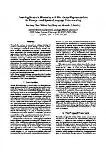
Figure 1: Dependency schema of a set of rooted subgraphs of degree 1 ((a), (d)), 2 ((b)) and 3 ((c)) in an Android malware’s API dependency graph. The root nodes are marked with a star. Graph (b) can be derived from (a) by adding a node and an edge. Graph (c) can be derived from (b) in a similar fashion. Graph (d) is highly dissimilar from all the other graphs and is not readily derivable from any of them.
lar and widely adopted approaches to measure similarities among graphs [3, 4, 6, 7, 14]. A Graph kernel measures the similarity between a pair of graphs by recursively decomposing them into atomic substructures (e.g., walk [3], shortest paths [4], graphlets [7] etc.) and defining a similarity function over the substructures (e.g., number of common substructures across both graphs). This makes the kernel function correspond to an inner product over substructures in reproducing kernel Hilbert space (RKHS). Formally, for a given graph G, let Φ(G) denote a vector which contains counts of atomic substructures, and h·, ·iH denote a dot product in a RKHS H. Then, the kernel between two graphs G and G0 is given by K(G, G0 ) = hΦ(G), Φ(G0 )iH
(1)
From an application standpoint, the kernel matrix K that represents the pairwise similarity of graphs in the dataset (calculated using eq. (1)) could be used in conjunction with kernel classifiers (e.g., Support Vector Machine (SVM)) and relational data clustering algorithms to perform graph classification and clustering tasks, respectively.
1.1
Limitations of Existing Graph Kernels
However, as noted in [7, 14], the representation in eq. (1) does not take two important observations into account.
ACM ISBN 978-1-4503-2138-9. DOI: 10.1145/1235
• (L1) Substructure Similarity. Substructures that are used to compute the kernel matrix are not independent. To illustrate this, lets consider the Weisfeiler-Lehman (WL)
kernel [6] which decomposes graphs into rooted subgraphs1 . These subgraphs encompass the neighbourhood of certain degree around the root node. Understandably, these subgraphs exhibit strong relationships among them. That is, a subgraph with second degree neighbours of the root node could be arrived at by adding a few nodes and edges to its first degree counterpart. We explain this with an example presented in Fig. 1. The figure illustrates APIdependency subgraphs from a well-known Android malware called DroidKungFu (DKF) [18]. These subgraph portions of DKF involves in leaking users’ private information (i.e., IMEI number) over the internet and sending premium-rates SMS without her consent. Sub-figures (a), (b) and (c) represent subgraphs of degree 1, 2 and 3 around the root node getSystemServices, respectively. Evidently, these subgraphs exhibit high similarity among one another. For instance, subgraph (c) could be derived from subgraph (b) by adding a node and an edge, which in turn could be derived from subgraph (a) in a similar fashion. However, the WL kernel, by design ignores these subgraph similarities and considers each of the subgraphs as individual features. Other kernels such as random walk and shortest path kernels also make similar assumptions on their respective substructures’ similarities. • (L2) Diagonal Dominance. Since graph kernels regard these substructures as separate features, the dimensionality of the feature space often grows exponentially with the number of substructures. Consequently, only a few substructures will be common across graphs. This leads to diagonal dominance, that is, a given graph is similar to itself but not to any other graph in the dataset. This leads to poor classification/clustering accuracy.
1.2
Existing Solution: Deep Graph Kernels
To alleviate these problems Yanardag and Vishwanathan [7], recently proposed an alternative kernel formulation termed as Deep Graph Kernel (DGK). Unlike eq. (1), DGK captures the similarities among the substructures with the following formulation: K(G, G0 ) = Φ(G)T MΦ(G0 )
(2)
where M represents a |V| × |V| positive semi-definite matrix that encodes the relationship between substructures and V represents the vocabulary of substructures obtained from the training data. Therefore, one can design a M matrix that respects the similarity of the substructure space. Learning representation of substructures. In DGK [7], the authors used representation learning (deep learning) techniques inspired by the work of Mikolov et al. [15] to learn vector representations (aka embeddings) of substructures. Subsequently, these substructure embeddings were used to compute M and the same is used in eq (2) to arrive at the deep learning variants of several well-known kernels such as WL, graphlet and shortest path kernels. Context. In order to facilitate unsupervised representation learning on graph substructures, the authors of [7] defined a notion of context among these substructures. Substructures that co-occur in the same context tend to have 1 The WL kernel models the subgraph around a root node as a tree (i.e., without cycles) and hence is referred as WL subtree kernel. However since the tree represents a rooted subgraph, we refer to the rooted subgraph as the substructure being modeled in WL kernel, in this work.
high similarity. For instance, in the case of rooted subgraphs, all the subgraphs that encompass same degree of neighbourhood around the root node are considered as cooccurring in the same context (e.g., all degree-1 subgraphs are considered to be in the same context). Subsequently, embedding learning task’s objective is designed to make the embeddings of substructures that occur in the same context similar to one another. Thus defining the correct context is of paramount importance to build high quality embeddings. Deep WL Kernel. Through their experiments the authors demonstrated that the deep learning variant of WL kernel constructed using the above-said procedure achieved state-of-the-art performances on several datasets. However, we observe that, in their approach to learn subgraph embeddings, the authors make three novice assumptions that lead to three critical problems: • (A1) Only rooted subgraphs of same degree are considered (d) as co-occurring in the same context. That is, if DG = (d) (d) {sg1 , sg2 , ...} is a multi-set of all degree d subgraphs in (d) (d) graph G, [7] assumes that any two subgraphs sgi , sgj (d)
∈ DG co-occur in the same context irrespective of the length (or number) of path(s) connecting them or whether they share the same nodes/edges. For instance, in the case of Android malware subgraphs in Fig. 1, [7] assumes that only subgraphs (a) and (d) are in the same context and are possibly similar as they both are degree-1 subgraphs. However in reality, they share nothing in common and are highly dissimilar. This assumption makes subgraphs that do not co-occur in the same graph neighbourhood to be in the same context and thus similar (problem 1). • (A2) Any two rooted subgraphs of different degrees never co-occur in the same context. That is, two subgraphs (d0 ) (d) (d0 ) (d) ∈ DG (where d 6= d0 ) never sgi ∈ DG and sgj co-occur in the same context irrespective of the length (or number) of path(s) connecting them or whether they share the same nodes/edges. For instance, in Fig. 1, subgraphs (a), (b) and (c) are considered not co-occurring in the same context as they belong to different degree neighbourhood around the root node. Hence, [7] incorrectly biases them to be dissimilar. This assumption makes subgraphs that co-occur in the same neighbourhood not to be in the same context and thus dissimilar (problem 2). (d)
• (A3) Every subgraph (sgr ) in any given graph has exactly same number of subgraphs in its context. This assumption clearly violates the topological neighbourhood structure in graphs (problem 3). Through our thorough analysis and experiments we observe that these assumptions led [7] to building relatively low quality subgraph embeddings. Consequently, this reduces the classification and clustering accuracies when [7]’s deep WL kernel is deployed. This motivates us to address these limitations and build better subgraph embeddings, in order to achieve higher accuracy.
1.3
Our Approach
In order to learn accurate subgraph embeddings, we address each of the three problems introduced in the previous subsection. We make two main contributions through our subgraph2vec framework to solve these problems: • We extend the WL relabeling strategy [6] (used to relabel the nodes in a graph encompassing its breadth-first neigh-
Table 1: Representation Learning from Graphs
bourhood) to define a proper context for a given subgraph. (d) For a given subgraph sgr in G with root r, subgraph2vec considers all the rooted subgraphs (up to a certain degree) (d) of neighbours of r as the context of sgr . This solves problems 1 and 2. • However this context formation procedure yields radial contexts of different sizes for different subgraphs. This renders the existing representation learning models such as the skipgram model [15] (which captures fixed-length linear contexts) unusable in a straight-forward manner to learn the representations of subgraphs using its context, thus formed. To address this we propose a modification to the skipgram model enabling it to capture varying length radial contexts. This solves problem 3. Experiments. We determine subgraph2vec’s accuracy and efficiency in both supervised and unsupervised learning tasks with several benchmark and large-scale real-world datasets. Also, we perform comparative analysis against several state-of-the-art graph kernels. Our experiments reveal that subgraph2vec achieves significant improvements in classification/clustering accuracy over existing kernels. Specifically, on two real-world program analysis tasks, namely, code clone and malware detection, subgraph2vec outperforms state-of-the-art kernels by more than 17% and 4%, respectively. Contributions. We make the following contributions: • We propose subgraph2vec, an unsupervised representation learning technique to learn latent representations of rooted subgraphs present in large graphs (§5). • We develop a modified version of the skipgram language model [15] which is capable of modeling varying length radial contexts (rather than fixed-length linear contexts) around target subgraphs (§5.2). • We discuss how subgraph2vec’s representation learning technique would help to build the deep learning variant of WL kernel (§5.3). • Through our large-scale experiments on several benchmark and real-world datasets, we demonstrate that subgraph2vec could significantly outperform state-of-the-art graph kernels (incl. [7]) on graph classification and clustering tasks (§6).
2.
RELATED WORK
The closest work to our paper is Deep Graph Kernels [7]. Since we have discussed it elaborately in §1, we refrain from discussing it here. Recently, there has been significant interest from the research community on learning representations of nodes and other substructures from graphs. We list the prominent such works in Table 1 and show how our work compares to them in-principle. Deep Walk [8] and node2vec [10] intend to learn node embeddings by generating random walks in a single graph. Both these works rely on existence of node labels for at least a small portion of nodes and take a semi-supervised approach to learn node embeddings. Recently proposed Patchy-san [9] learns node and subgraph embeddings using a supervised convolutional neural network (CNN) based approach. In contrast to these three works, subgraph2vec learns subgraph embeddings (which includes node embeddings) in an unsupervised manner.
Learning node subgraph Context used for Paradigm vector vector rep. learning Fixed-length Deep Walk [8] Semi-sup random walks Fixed-Length biased node2vec [10] Semi-sup random walks Receptive field of sequence Patchy-san [9] Sup of neighbours of nodes Deep Graph Subgraphs occurring [7] Unsup Kernels at same degree Subgraphs of different degrees occurring in the subgraph2vec Unsup same local neighbourhoods Solution
In general, from a substructure analysis point of view, research on graph kernel could be grouped into three major categories: kernels for limited-size subgraphs [12], kernels based on subtree patterns [6] and kernels based on walks [3] and paths [4]. subgraph2vec is complementary to these existing graph kernels where the substructures exhibit reasonable similarities among them.
3.
PROBLEM STATEMENT
We consider the problem of learning distributed representations of rooted subgraphs from a given set of graphs. More formally, let G = (V, E, λ), represent a graph, where V is a set of nodes and E ⊆ (V × V ) be a set of edges. Graph G is labeled2 if there exists a function λ such that λ : V → `, which assigns a unique label from alphabet ` to every node v ∈ V . Given G = (V, E, λ) and sg = (Vsg , Esg , λsg ), sg is a sub-graph of G iff there exists an injective mapping µ : Vsg → V such that (v1 , v2 ) ∈ Esg iff (µ(v1 ), µ(v2 )) ∈ E. Given a set of graphs G = {G1 , G2 , ..., Gn } and a positive integer D, we intend to extract a vocabulary of all (rooted) subgraphs around every node in every graph Gi ∈ G encompassing neighbourhoods of degree 0 ≤ d ≤ D, such that SGvocab = {sg1 , sg2 , ...}. Subsequently, we intend to learn distributed representations with δ dimensions for every subgraph sgi ∈ SGvocab . The matrix of representations (embeddings) of all subgraphs is denoted as Φ ∈ R|SGvocab |×δ . Once the subgraph embeddings are learnt, they could be used to cater applications such as graph classification, clustering, node classification, link prediction and community detection. They could be readily used with classifiers such as CNNs and Recurrent Neural Networks. Besides this, these embeddings could be used to make a graph kernel (as in eq(2)) and subsequently used along with kernel classifiers such as SVMs and relational data clustering algorithms. These use cases are elaborated later in §5.4 after introducing the representation learning methodology.
4.
BACKGROUND: LANGUAGE MODELS
Our goal is to learn the distributed representations of subgraphs extending the recently proposed representation learning and language modeling techniques for multi-relational data. In this section, we review the related background in language modeling. Traditional language models. Given a corpus, the traditional language models determine the likelihood of a sequence of words appearing in it. For instance, given a sequence of words {w1 , w2 , ..., wT }, n-gram language model 2 For graphs without node labels, we follow the procedure mentioned in [6] and label nodes with their degree.
targets to maximize the following probability: P r(wt |w1 , ..., wt−1 )
Algorithm 1: subgraph2vec (G, D, δ, e)
Meaning, they estimate the likelihood of observing the target word wt given n previous words (w1 , ..., wt−1 ) observed thus far. Neural language models. The recently developed neural language models focus on learning distributed vector representation of words. These models improve traditional ngram models by using vector embeddings for words. Unlike n-gram models, neural language models exploit the of the notion of context where a context is defined as a fixed number of words surrounding the target word. To this end, the objective of these word embedding models is to maximize the following log-likelihood: T X
logP r(wt |wt−c , ..., wt+c )
(4)
Skip Gram
The skipgram model maximizes co-occurrence probability among the words that appear within a given context window. Give a context window of size c and the target word wt , skipgram model attempts to predict the words that appear in the context of the target word, (wt−c , ..., wt−c ). More precisely, the objective of the skipgram model is to maximize the following loglikelihood, log P r(wt−c , ..., wt+c |wt )
(5)
t=1
3 4 5 6 8
Π−c≤j≤c,j6=0 P r(wt+j |wt )
(6)
Here, the contextual words and the current word are assumed to be independent. Furthermore, P r(wt+j |wt ) is defined as: 0
exp(ΦTwt Φwt+j ) PV 0 T w=1 exp(Φwt Φw )
begin SGvocab = BuildSubgraphVocab(G) //use Algorithm 2 Initialization: Sample Φ from U |SGV ocab|×δ for e = 0 to e do G = Shuffle (G) for each Gi ∈ G do for each v ∈ Vi do for d = 0 to D do (d) sgv := GetWLSubgraph(v, Gi , d)
(7)
where Φw and Φw 0 are the input and output vectors of word w.
Negative Sampling
The posterior probability in eq. (6) could be learnt in several ways. For instance, a novice approach is to use a classifier like logistic regression. This is prohibitively expensive if the vocabulary of words is very large. Negative sampling is an efficient algorithm that is used to alleviate this problem and train the skipgram model. Negative sampling selects the words that are not in the context at random instead of considering all words in the vocabulary. In other words, if a word w appears in the context of another word w0 , then the vector embedding of w is closer to that of w0 compared to any other randomly chosen word from the vocabulary. Once skipgram training converges, semantically similar words are mapped to closer positions in the embedding space
(d)
RadialSkipGram (Φ, sgv , Gi , D)
10
11
return Φ
revealing that the learned word embeddings preserve semantics. An important intuition we extend in subgraph2vec is to view subgraphs in large graphs as words that are generated from a special language. In other words, different subgraphs compose graphs in a similar way that different words form sentences when used together. With this analogy, one can utilize word embedding models to learn dimensions of similarity between subgraphs. The main expectation here is that similar subgraphs will be close to each other in the embedding space.
5.
where the probability P r(wt−c , ..., wt+c ) is computed as
4.2
2
9
where (wt |wt−c , ..., wt+c ) are the context of the target word wt . Several methods are proposed to approximate eq. (4). Next, we discuss one such a method that we extend in our subgraph2vec framework, namely Skipgram models [15].
T X
1
7
t=1
4.1
input : G = {G1 , G2 , ..., Gn }: set of graphs such that each graph Gi = (Vi , Ei , λi ) from which embeddings are learnt D: Maximum degree of subgraphs to be considered for learning representations. This will produce a vocabulary of subgraphs, SGvocab = {sg1 , sg2 , ...} from all the graphs in G δ: number of dimensions (embedding size) e: number of epochs output: Matrix of vector representations of subgraphs Φ ∈ R|SGvocab |×δ
(3)
METHOD: LEARNING SUB-GRAPH REPRESENTATIONS
In this section we discuss the main components of our subgraph2vec algorithm (§5.2), how it enables making a deep learning variant of WL kernel (§5.3) and some of its usecases in detail (§5.4).
5.1
Overview
Similar to the language modeling convention, the only required input is a corpus and a vocabulary of subgraphs for subgraph2vec to learn representations. Given a dataset of graphs, subgraph2vec considers all the neighbourhoods of rooted subgraphs around every rooted subgraph (up to a certain degree) as its corpus, and set of all rooted subgraphs around every node in every graph as its vocabulary. Subsequently, following the language model training process with the subgraphs and their contexts, subgraph2vec learns the intended subgraph embeddings.
5.2
Algorithm: subgraph2vec
The algorithm consists of two main components; first a procedure to generate rooted subgraphs around every node in a given graph (§5.2.1) and second the procedure to learn embeddings of those subgraphs (§5.2.2). As presented in Algorithm 1 we intend to learn δ dimensional embeddings of subgraphs (up to degree D) from all the graphs in dataset G in e epochs. We begin by building a vocabulary of all the subgraphs, SGvocab (line 2) (using
Algorithm 2: GetWLSubgraph (v, G, d) input : v: Node which is the root of the subgraph G = (V, E, λ): Graph from which subgraph has to be extracted d: Degree of neighbours to be considered for extracting subgraph output: sgv(d) : rooted subgraph of degree d around node v 1 2
3 4 5
begin (d) sgv = {} if d = 0 then (d) sgv := λ(v)
5.2.2
6
Mv
:= {GetWLSubgraph(v 0 , G, d − 1) | v 0 ∈ Nv }
7
(d) sgv
:= sgv ∪ GetWLSubgraph
(d)
(d)
(v, G, d − 1) ⊕ sort(Mv ) 8
(d)
return sgv
(d)
Algorithm 3: RadialSkipGram (Φ, sgv , G, D) 1 2 3 4 5 6
7 8 9
begin (d) contextv = {} for v 0 ∈ Neighbours(G, v) do for ∂ ∈ {d − 1, d, d + 1} do if (∂ ≥ 0 and ∂ ≤ D) then (d) (d) contextv = contextv ∪ 0 GetWLSubgraph(v , G, ∂) (d)
for each sgcont ∈ contextv do (d) J(Φ) = −log Pr (sgcont |Φ(sgv )) ∂J Φ = Φ − α ∂Φ
Algorithm 2). Then the embeddings for all subgraphs in the vocabulary (Φ) is initialized randomly (line 3). Subsequently, we proceed with learning the embeddings in several epochs (lines 4 to 10) iterating over the graphs in G. These steps represent the core of our approach and are explained in detail in the two following subsections.
5.2.1
Radial Skipgram (d)
else Nv := {v 0 | (v, v 0 ) ∈ E} (d)
the graph 1(c) as the complete graph from which we intend to get the degree 0, 1 and 2 subgraph around the root node HttpURL.init. Subjecting these inputs to Algorithm 2, we get subgraphs {HttpURL.init}, {HttpURL.init -> OpenConnection} and {HttpURL.init -> OpenConnection -> Connect} for degrees 0, 1 and 2, respectively.
Extracting Rooted Subgraphs
To facilitate learning its embeddings, a rooted subgraph (d) sgv around every node v of graph Gi is extracted (line 9). This is a fundamentally important task in our approach. To extract these subgraphs, we follow the well-known WL relabeling process [6] which lays the basis for the WL kernel and WL test of graph isomorphism [6, 7]. The subgraph extraction process is explained separately in Algorithm 2. The algorithm takes the root node v, graph G from which the subgraph has to be extracted and degree of the intended subgraph d as inputs and returns the intended subgraph (d) sgv . When d = 0, no subgraph needs to be extracted and hence the label of node v is returned (line 3). For cases where d > 0, we get all the (breadth-first) neighbours of v in Nv (line 5). Then for each neighbouring node, v 0 , we get (d) its degree d − 1 subgraph and save the same in list Mv (line 6). Finally, we get the degree d − 1 subgraph around the root node v and concatenate the same with sorted list (d) (d) Mv to obtain the intended subgraph sgv (line 7). Example. To illustrate the subgraph extraction process, lets consider the examples in Fig. 1. Lets consider
Once the subgraph sgv , around the root node v is extracted, Algorithm 1 proceeds to learn its embeddings with the radial skip gram model (line 10). Similar to the vanilla skipgram algorithm which learns the embeddings of a target word from its surrounding linear context in a given document, our approach learns the embeddings of a target subgraph using its surrounding radial context in a given graph. The radial skipgram procedure is presented in Algorithm 3. Modeling the radial context. The radial context around a target subgraph is obtained using the process explained below. As discussed previously in §4.1, natural language text have linear co-occurrence relationships. For instance, skipgram model iterates over all possible collocations of words in a given sentence and in each iteration it considers one word in the sentence as the target word and the words occurring in its context window as context words. This is directly usable on graphs if we model linear substructures such as walks or paths with the view of building node representations. For instance, Deep Walk [8] uses a similar approach to learn a target node’s representation by generating random walks around it. However, unlike words in a traditional text corpora, subgraphs do not have a linear co-occurrence relationship. Therefore, we intend to consider the breadth-first neighbours of the root node as its context as it directly follows from the definition of WL relabeling process. To this end, we define the context of a degree-d subgraph (d) sgv rooted at v, as the multiset of subgraphs of degrees d − 1, d and d + 1 rooted at each of the neighbours of v (lines 2-6 in Algorithm 3). Clearly this models a radial context rather than a linear one. Note that we consider subgraphs of degrees d−1, d and d+1 to be in the context of a subgraph of degree d. This is because, as explained with example earlier in §1.1, a degree-d subgraph is likely to be rather similar to subgraphs of degrees that are closer to d (e.g., d − 1, d + 1) and not just degree-d subgraphs only. Vanilla Skip Gram. As explained previously in §4.1, the vanilla skipgram language model captures fixed-length linear contexts over the words in a given sentence. However, for learning a subgraph’s radial context arrived at line 6 in Algorithm 3, the vanilla skipgram model could not be used. Hence we propose a minor modification to consider a radial context as explained below. Modification. The embedding of a target subgraph, (d) (d) sgv , with context contextv is learnt using lines 7 - 9 in Algorithm 3. Given the current representation of target sub(d) graph Φ(sgv ), we would like to maximize the probability of every subgraph in its context sgcont (lines 8 and 9). We can learn such posterior distribution using several choices of classifiers. For example, modeling it using logistic regression would result in a huge number of labels that is equal to |SGvocab |. This could be in several thousands/millions in the case of large graphs. Training such models would require large amount of computational resources. To alleviate this bottleneck, we approximate the probability distribution using the negative sampling approach.
5.2.3
Table 2: Benchmark dataset statistics
Negative Sampling
Dataset
# samples
# nodes
# distinct
(avg.) node labels Given that sgcont ∈ SGvocab and |SGvocab | is very large, MUTAG 188 17.9 7 (d) calculating P r(sgcont |Φ(sgv )) in line 8 is prohibitively exPTC 344 25.5 19 pensive. Hence we follow the negative sampling strategy PROTEINS 1113 39.1 3 NCI1 4110 29.8 37 (introduced in §4.2) to calculate above mentioned posteNCI109 4127 29.6 38 rior probability. In our negative sampling phase for every training cycle of Algorithm 3, we choose a fixed number of subgraphs (denoted as negsamples) as negative samdegree 0 are considered, subgraph2vec provides node embedples and update their embeddings as well. Negative samdings similar to Deep Walk [8] and node2vec [10]). Hence ples adhere to the following conditions: if negsamples = other tasks such as node classification, community detec{sgneg1 , sgneg2 , ...}, then negsamples ⊂ SGvocab , |negsamples|