Geosciences Journal Vol. 12, No. 2, p. 107 − 122, June 2008 DOI 10.1007/s12303-008-0013-x
Simulating complex flow and transport dynamics in an integrated surfacesubsurface modeling framework
}
Edward A. Sudicky* Jon P. Jones Department of Earth and Environmental Sciences, University of Waterloo, Waterloo, Ontario, Young-Jin Park Canada N2L 3G1 Andrea E. Brookfield Dennis Colautti
ABSTRACT: A fully-integrated surface-subsurface flow and transport model is applied to a 17 km2 subcatchment of the Laurel Creek Watershed within the Grand River basin in Southern Ontario, Canada. Through past and ongoing field studies, the subcatchment is reasonably well characterized and is being monitored on an ongoing basis. In addition to diverse land-usage and surface cover and more than 65 m of topographic relief, the watershed is underlain by a complex interconnected sequence of sand and gravel aquifers that are separated by discontinuous clayey aquitards. A steady-state condition was achieved in the model by calibrating the subsurface flow field to 16 observation wells where long-term hydraulic head data were available, while simultaneously establishing a level of baseflow discharge on the surface regime approximating the level observed at the beginning of the transient simulation period. The model is then subjected to several hundred hours of rainfall data and the resulting discharge hydrographs are compared with the measured hydrographs. The calculated subsurface hydraulic head distribution and surficial rainfallrunoff responses, respectively, were shown to agree moderately well with those observed in the system during this period. The impact of an upland surficial contaminant source discharging along a reach of a small stream within the subcatchment was also examined. Results showed that short-duration, high-intensity concentration peaks were not captured if annual or monthly average rainfall was used as input. The hydraulic head and concentration variations due to short-duration rainfall variations showed a muted response with increasing depth below the streambed due to the natural smoothing in the hydraulic response and to dispersion and diffusion of the solute, respectively. Discrete daily precipitation events were also found to cause rapid changes in the calculated water and solute exchange fluxes. The variability and sensitivity of these near-stream processes to the temporal resolution of rainfall input, specifically the concentration and solute exchange flux responses, may be significant in the prediction of health risks to aquatic habitats. Overall, it is concluded that the model is capable of reproducing surface and subsurface hydrodynamic processes at the subcatchment scale although the results could be better through improved parameterization of the subcatchment and the manner in which the model simulates evapotranspiration processes. Key words: surface-subsurface, fully-integrated, Laurel Creek, nearstream processes
*Corresponding author:
[email protected]
1. INTRODUCTION Although the ‘blueprint’ for physically-based, surfacesubsurface models was first proposed over three and a half decades ago (Freeze and Harlan, 1969), its use has only become widespread in the past 15 years with the advent of inexpensive and powerful desktop computers. The majority of the models developed to date within this framework link components of the surface and subsurface regimes together using externally-coupled/time-lagged schemes (e.g., Abbott et al., 1986; Refsgaard and Storm, 1996; Ewen et al., 2000) or iteratively-coupled approaches (e.g., Pinder and Sauer, 1971; Freeze, 1972a, b; Morita and Yen, 2002) with respect to the compatibility of land surface interface fluxes or pressure heads. An alternative to these approaches is to solve the surface, subsurface, and interface fluxes simultaneously. This method, referred to as the fully-integrated or fully-coupled approach, is both theoretically and aesthetically more satisfying due to the elimination of the “artificial” boundary condition between the surface-subsurface interface that exists when applying externally- or iteratively-coupled approaches. Moreover, the fully-integrated approach has also been shown to outperform externally- and iteratively-coupled approaches (in terms of computational efficiency) in systems with highly nonlinear rainfall-runoff responses (Panday and Huyakorn, 2004). The fully-integrated approach, originally implemented by Brown (1995) is relatively new; however, a number of physically-based, distributed models are now incorporating the numerical solution technique (e.g., Hydrogeologic, 2000), including the models developed at the University of Waterloo such as the Integrated Hydrology Model (InHM: a first generation of fully-integrated surface-subsurface numerical simulator) (VanderKwaak, 1999) and the HydroGeoSphere (a second generation of fully-integrated numerical model) (Therrien et al., 2004). Fully-integrated surface-subsurface models have already been successfully applied to the simulation of discrete precipitation events at the 0.1 km2 R-5 subcatchment near Chickasha, Oklahoma (VanderKwaak and Loague, 2001; Loague
108
Edward A. Sudicky, Jon P. Jones, Young-Jin Park, Andrea E. Brookfield, and Dennis Colautti
and VanderKwaak, 2002; Loague et al., 2005) and to the evaluation of event and pre-event water contribution to stream flow generation (Jones et al., 2006). In this study, fully-integrated approach will be applied to a hydrologically complex but reasonably well-characterized 17 km2 subcatchment of the Laurel Creek Watershed located in Southern Ontario, Canada. The objectives of the current work are: (1) to perform an analysis of the ability of the fully-coupled model to reproduce subsurface and surface flow characteristics observed in the subcatchment under steady-state and transient conditions, respectively, and (2) to analyze the effect of precipitation events on near-stream flow and transport processes. These objectives are accomplished by first calibrating the subsurface hydraulic head distribution of the system to 16 observations wells where long-term average hydraulic head data are available, while simultaneously establishing a level of baseflow discharge in the drainage network on the surface comparable to that observed in the subcatchment during the transient simulation period. Next, the system is subjected to several hundred hours of precipitation data obtained at a weather station located near the subcatchment and the resulting discharge hydrographs are compared with the measured rainfall-runoff responses. The model of the subcatchment is then used to evaluate the effect of different temporal precipitation averages on nearstream processes when a surficially-applied contaminant plume migrates through the subsurface and discharges into a stream. 2. FULLY-INTEGRATED NUMERICAL MODEL The fully-integrated numerical model developed at the University of Waterloo (VanderKwaak, 1999; Therrien et al., 2004) is a control-volume finite element model capable of simulating surface-subsurface watershed flow and solute
Fig. 1. Location of the Laurel Creek Watershed subcatchment.
transport processes in a single three-dimensional framework. Transient overland and open channel flow on the land surface is described using the two-dimensional diffusionwave approximation of the St. Venant equation while a three-dimensional variably saturated form of the Richards’ equation governs flow processes in the subsurface. Full coupling of the surface and subsurface flow regimes is accomplished by mutual water and solute exchange flux terms which allow the model to simultaneously solve one system of nonlinear discrete equations describing flow and tracer transport in both flow regimes. For a complete description of the model capabilities, the reader is directed to VanderKwaak (1999) and Therrien et al. (2004). 3. STUDY AREA The study area consists of a 17 km2 subcatchment of the Laurel Creek Watershed within the Grand River basin, which is located in Southern Ontario, Canada (Fig. 1). This site was chosen because the Laurel Creek Watershed has been intensely studied for over 30 years and is monitored on an ongoing basis (Karrow, 1974; Ross, 1986; Farvolden et al., 1987; Terraaqua Ltd., 1993; Paloschi, 1993; Gautry, 1996; Radcliffe, 2000). The subcatchment is drained by Laurel Creek, whose average stream depths range from 0.1 to 2.0 meters within the study area, as well as a number of smaller intermittent tributaries. The land surface is hummocky and contains a number of wetlands where the water table intersects the land surface. Surface elevation within the study area ranges from a maximum of 410 meters above sea level (masl) along the southern boundaries of the subcatchment to a minimum of 345 masl near the subcatchment outlet, yielding 65 m of topographic relief within the system. The climate of the subcatchment is considered semi-humid and receives an average of 908 mm
Flow and transport in an integrated modeling framework
of precipitation (rainfall and water equivalent snow) per year (Environment Canada, 2003). Land use within the subcatchment varies although it is predominantly rural. The subcatchment’s overburden is comprised of 80 to 100 m of unconsolidated glacial sediments formed by interlobate glacial activity during the late Wisconsin stage (Karrow, 1989). The stratigraphy of the overburden consists of a laterally discontinuous sequence of unconsolidated silty and clayey glacial tills that act as aquitards. These aquitards are separated by aquifers composed of glaciofluvial sand and reworked tills. Because the aquitards are discontinuous, a number of hydraulic connections exist between the shallow and deep groundwater systems, thus generating a very complex subsurface flow system. The subcatchment is bounded underneath by the Salina Formation. The Salina Formation is of the late Silurian period and consists of 120 m to 180 m of interbedded grey to green shale, mudstone, brown dolomite, gypsum and salt (Karrow, 1993). Karstic and fractured systems are common throughout the Salina Formation (Gautry, 1996). The bedrock topography has been mapped several times over the past 30 years, most recently by Holden et al. (1993), and is characterized by a rolling surface. The Salina Formation dips gently westward towards the Michigan Basin (Karrow, 1987). 4. PHYSICAL SYSTEM A 25-meter Digital Elevation Model (DEM) obtained from the Grand River Conservation Authority of Ontario was used to define a 2D triangular-element mesh representing the top of the model domain (ground surface) as well as the lateral extents of the subcatchment. The mesh was designed such that element dimensions near the streams have an average plan view length of about 10 m, while elements further away from the drainage network grade out to approximately 75 m. This type of mesh allows a more accurate rendering of the near-stream hydrodynamic processes, while reducing computational effort in terms of spatial discretization in less hydrologically active areas. The main channel of the drainage network and a number of its tributaries were incised into the surface mesh by lowering the stream nodes 0.2 m. This incision process was done to generate wetted-perimeter channel widths more akin to the widths observed in the drainage network of the subcatchment. A digital map of land usage was interpolated onto the surface mesh and five distinct land-use categories were identified. The subcatchment is predominantly rural, although there are limited urbanized, wetlands and forested portions. Each land-use category was assigned a Manning’s surface roughness coefficient extracted from tables provided in McCuen (1989).
109
In the integrated hydrologic simulator used for this study, surface water flow is simulated using a 2-D mesh, which is superimposed onto a 3D finite-element mesh used to simulate subsurface flow. The top of the 3D mesh is coincident with the 2D mesh such that dual nodes exist at the surfacesubsurface interface. Twenty layers separate the surface and the base of the 3D mesh, which is defined by the bedrock surface. Vertical discretization in the 3D mesh is on the order of 0.5 m for the two layers adjacent to the land surface and increases to a maximum of approximately 8.5 m at depth. The finer level of vertical discretization in the shallow subsurface was used to better capture surface watergroundwater interactions occurring near the land surface interface. Conversely, the coarser discretization levels deeper in the subsurface help reduce the overall computational effort while remaining sufficiently fine enough to accurately represent the subsurface hydrostratigraphy as interpreted from borehole logs. The bottom and side boundaries of the domain are assumed to be impermeable with respect to both surface and subsurface flow. Outflow is only allowed through three nodes in the 2D surface mesh, which were chosen along the segment of the surficial domain where the subcatchment discharges into the lower portion of the Laurel Creek Watershed. This discharge point coincides with the Erbsville gauge station (located in Fig. 1), thereby providing a calibration point for the calculated discharge hydrographs. A nonlinear critical-depth boundary condition is applied at these outflow nodes which constrains neither the flow rate nor the surface water depth. Instead, the surface outflow (i.e., the stream discharge leaving the domain) is allowed to vary naturally throughout a given simulation period depending on the calculated depth of water at the outlet. The subsurface hydraulic conductivity distribution was mapped onto the three-dimensional subsurface mesh from the calibrated results of a previous regional study conducted by Radcliffe (2000) that, in turn, was a refinement of the earlier work of Martin (1994) and Martin and Frind (1998). The configuration of the subsurface hydraulic conductivity field was originally extracted from over 1100 borehole logs provided by the Ontario Ministry of the Environment. The resulting hydraulic conductivity pattern shows a complex interconnected sequence of sand- and gravel-dominated aquifers separated by discontinuous aquitards. A veneer of topsoils was superimposed onto the top meter of the subsurface hydraulic conductivity field. A digital soil map provided by Environment Canada contained the locations and name of each soil series as determined from previous soil survey studies. The hydrological parameters assigned to each soil series were estimated using pedotransfer functions based on the textural data found in the Waterloo County Soil Survey (Presant and Wickland, 1971). Inspection of the previous work of Lee (1967) indicated that the penetration depths of the topsoils in the subcatchment are
110
Edward A. Sudicky, Jon P. Jones, Young-Jin Park, Andrea E. Brookfield, and Dennis Colautti
all relatively shallow and that a uniform soil depth of one meter would be reasonably representative of the actual distribution. 5. FLOW SIMULATION A uniform net rainfall rate was applied to the surface of the initially saturated system until steady-state equilibrium was achieved in both the surface and subsurface flow regimes. The rainfall rate applied to the surface of the system was chosen such that the model-calculated volumetric streamflow rate exiting the system under steady-state conditions equalled the baseflow observed at the beginning of the transient simulation period discussed below (i.e., 0.04 m3/s). Recalling that water can only exit the system at the discharge point, this net rainfall input, 7.13 cm/yr, represents the actual mean rainfall rate required to generate the observed level of baseflow minus the effects of evapotranspiration. The computed steady-state drainage network is presented alongside the observed drainage network in Figure 2. Note that the location of the drainage network within the subcatchment was not part of the parameterization process. Instead, while the system equilibrated, the genesis of the surface drainage network was arrived at by the movement of water within and between the surface and subsurface flow regimes. Also note that the simulation does not a priori assume any streamflow generation mechanisms because, by its formulation, infiltration excess overland flow, baseflow and subsurface storm flow processes are all implicitly represented (VanderKwaak, 1999; VanderKwaak and Loague, 2001). Therefore, during the course of a simulation, it determines where water infiltrates, exfiltrates,
Fig. 2. (a) Observed and (b) calculated drainage networks.
or forms surface water in drainage channels or wetlands. As can be seen in Figure 2, the calculated location and extent of the main channel of Laurel Creek corresponds reasonably well with the observed channel (denoted in dark blue on the observed drainage network in Figure 2) although the observed channel extends further eastward. Similarly, there is reasonable agreement between the locations and extents of a number the minor tributaries present in the subcatchment and those calculated by the model. Although there are some discrepancies between the computed and observed drainage networks, it should be pointed out that the observed drainage network may contain a number of ephemeral water course features. To illustrate how the surface flow regimes are contributing to generating the calculated drainage network, steadystate water flow velocity vectors computed by the model were mapped onto the surface mesh (Fig. 3). As might be expected, the water flow velocity vectors on the surface mesh show that surface water in the upslope regions is flowing downgradient and converging towards the channels as a function of topography, soil infiltration capacity and antecedent moisture conditions and, once in the channel, moving downstream towards the discharge point of the subcatchment. The corresponding subsurface water flow velocity vectors indicate that water is infiltrating into the deeper subsurface in the topographically high areas away from the channels while exfiltration is occurring into the channels themselves and in the regions proximal to the channels. Note also that the relative density of the water flow velocity vectors under the channels reveals the rather strong level of interaction occurring between the surface and subsurface flow regimes which, in our opinion, re-enforces the notion
Flow and transport in an integrated modeling framework
111
Fig. 3. The yellow box shows the area expanded. Surface velocity vectors were mapped on the surface mesh.
Fig. 4. The distribution of total hydraulic head under steady-state conditions for the calibrated system.
that these types of problems are best simulated using fullyintegrated surface-subsurface approaches. The fully-integrated simulator requires an initial estimate of the water table position prior to initiating transient variably-saturated flow simulations. Although water table position information is not available at this time, long-term average hydraulic head measurements are available at 16 observation wells in the subcatchment. Observation nodes were emplaced in the subsurface mesh at the corresponding observation well locations for the purposes of calibrating the computed hydraulic head distribution. The calibration process was performed manually in an iterative fashion
whereby the hydraulic conductivity values of each lithofacies category were adjusted within physically realistic bounds until the best possible match was found between the simulated and observed heads. The calibrated hydraulic head distribution for the subsurface flow regime is shown in Figure 4. The distribution indicates that water is flowing in the subsurface away from topographic highs (corresponding to areas of greater hydraulic head) and converging towards the streams and lowland areas. Figure 4 also indicates convergence of subsurface flow towards the stream outlet. Although the hydraulic head distribution appears reasonable, there is only moderate agreement between the calculated hydraulic head values and the long-term average values determined from the observation wells (Fig. 5). Most of the discrepancies between the calculated and observed hydraulic heads are believed to be due to the zero-flux conditions assigned to the lateral boundaries of the system domain under the assumption that the surface and subsurface flow catchments coincide; however, as previous studies have indicated (e.g., Tiedeman et al., 1998), surface-water domain boundaries and groundwater divides often do not coincide. Another possible source of error between the calculated and observed hydraulic heads is uncertainty in the interpretation of the subsurface hydraulic conductivity data available from well logs and the spatial interconnectivity of the identified hydrostratigraphic units. The aquitards in the subcatchment are known to be highly discontinuous and exhibit numerous high conductivity connections between the shallow and deep subsurface flow systems (Martin and Frind, 1998). Additionally, there are currently no transient, spatially-distributed unsaturated moisture data
112
Edward A. Sudicky, Jon P. Jones, Young-Jin Park, Andrea E. Brookfield, and Dennis Colautti
Fig. 5. Calculated and observed hydraulic heads at 16 locations throughout the Laurel Creek Watershed subcatchment.
available to calibrate the unsaturated zone properties of the surficial soils. Such data are highly relevant for resolving the details of the spatial and temporal variability of the infiltration and recharge characteristics of the subcatchment. Once a steady-state initial condition was achieved, several hundred hours of actual discrete rainfall events (in 15 min increments) recorded at the University of Waterloo weather station (located in Fig. 1) were input into the model in order to assess the ability of the fully-integrated approach to reproduce observed transient rainfall-runoff responses. Note that, because the model cannot currently account for processes such as snowmelt, the transient rainfall-runoff simulations presented in this work are constrained to a time period (July 6 through September 24, 1999) where the effects of soil freezing and thawing and snowmelt are not a factor. To approximate the effects of evapotranspiration during the transient flow simulation, the intensities of the individual, discrete rainfall events were reduced until the computed rainfall-runoff responses provided the best match to the observed rainfall-runoff responses. For the transient simulation, the rainfall intensity rates were decreased by 40 % to provide this match (i.e., the input rainfall intensities were 60 % of the observed intensities). The resulting discharge hydrographs were then compared to responses observed at the Erbsville gauge station, where continuous monitoring data exists. The calculated and observed rainfall-runoff responses for the transient simulation period are shown in Figure 6. As can be seen in Figure 6, the computed discharge hydrograph reasonably matches the observed hydrograph, although the recession portions of a number of the peaks underpredict the corresponding observed recessions. This underprediction is believed to be due to the simplistic way in which the effects of evapotranspiration
Fig. 6. Calculated and observed rainfall-runoff responses for the transient period.
are being represented in the simulation. Because the effects of evapotranspiration were represented by uniformly lowering the rainfall intensity rates, as opposed to incorporating these effects directly into the governing flow equations, the simulated rainfall-runoff response will, by necessity, be impacted. For example, consider the direct overland runoff component of the system’s rainfall-runoff response to a single, relatively large, discrete rainfall event. Because the event’s actual intensity was lowered, the possibility exists that the infiltration capacity of the shallow subsurface will not be exceeded at various points in the system resulting in infiltration where overland runoff should have occurred, thereby impacting the calculated rainfall-runoff response in the manner shown in Figure 6. However, even when one takes these potential limitations into consideration, the overall level of agreement between the calculated and observed rainfall-runoff responses indicates that the model is able to capture the salient details of the interaction occurring between the surface and subsurface flow regimes in the subcatchment. 6. IMPACT OF A SURFICIAL CONTAMINANT SOURCE ON WATER QUALITY 6.1. Simulation Strategy and Steady-State Results Synthetic daily, monthly and annual precipitation data were generated for the subcatchment using the Hydraulic Evaluation of Landfill Performance (HELP) model’s weather generator (Schroeder et al., 1994). The HELP model generates precipitation as well as temperature and radiation data based on the longitude and latitude of the subcatchment. The average annual precipitation calculated for the subcatchment equals 2.3 mm/d and the total precipitation
Flow and transport in an integrated modeling framework
for a one year period is 840 mm. These values correspond reasonably well to historical rainfall data documented for the Waterloo region (Environment Canada, 2003). For each of the scenarios discussed in this study, a surficial contaminant source is placed on the land surface near the stream which forms a subsurface plume that discharges into the stream. The simulation strategy is as follows. First, a quasi-steady-state subsurface plume was simulated for a period of 30 years using the steady-state surface-subsurface flow system described above driven by the average annual precipitation as input (minus evapotranspiration). The concentrations in the stream, at the stream outlet as well as in the core of the subsurface plume were found to change by less than 0.001 percent/year after the 30 yr period. This quasi-steady-state scenario then served as the initial condition for subsequent transient flow and transport simulations of one-year duration in which synthetic precipitation rates were input on annual, monthly and daily time scales. Several observation nodes at a number of locations were used to monitor concentration, hydraulic heads and water and solute exchange flux variations over time. The locations of the surficial observation nodes are shown in Figure 7. These locations were selected on the basis of the direction and magnitude of water movement through the model domain, and because of their proximity to the stream. Node (A) is located at the base of the stream downslope from the contaminant source zone in an area where the stream is gaining water from the subsurface. Node (B) is also located where the plume intercepts the stream, but it is a region
113
where, on average, the stream is losing water to the subsurface. Node (C) is located downstream from where the subsurface plume intersects the stream and is in a region where the stream is gaining water from the subsurface. The outlet node was included in order to examine the hydrograph and concentration breakthrough for the entire subwatershed. The subsurface observation nodes (A1), (B1) and (C1) are located one meter below nodes (A), (B) and (C), respectively, while node (A10) is located 10 m below node (A). The location of the surficial contaminant source was chosen on the basis of the calculated steady-state groundwater flow patterns. The source location is in an upland region where infitration transports the contaminant from the land surface to the water table. Once the contaminant enters the saturated zone, it subsequently migrates towards the stream where it discharges both along a seepage face and though the stream bed into the surface water. The source zone comprises a quasi-rectangular 200 m by 300 m region and it is located approximately 500 m from the stream channel. The surficial source is conceptualized as being typical of a small field located in an upland region where agrochemicals might be applied. A constant concentration equal to 1.0 (i.e., C0) was applied on the land surface at the source. The contaminant is assumed to consist of a conservative, nonreactive tracer. The porous-medium transport parameters used in all of the simulations are as follows: a longitudinal dispersivity equal to 0.5 m, a horizontal transverse dispersivity of 0.05 m and
Fig. 7. Location of stream observation nodes (A), (B), (C) and channel outlet.
114
Edward A. Sudicky, Jon P. Jones, Young-Jin Park, Andrea E. Brookfield, and Dennis Colautti
Fig. 8. Concentration breakthrough curve at the channel outlet.
a vertical transverse dispersivity equal to 0.005 m. The surface water transport parameters use a longitudinal dispersivity of 1.0 m and a transverse dispersivity equal to 0.1 m. The freesolution diffusion coefficient of the tracer was assigned a
value of 1.2×10⁻⁹ m2/s. After 30 years of plume migration, the concentration at the channel outlet stabilized at a relative concentration, C/C0, of 4.48×10⁻³. The concentration breakthrough curve at the outlet is shown in Figure 8. Note that a relative concentration of 1.0×10⁻⁶ is attained at approximately 800 days (~2.2 years), after which time the concentrations steadily increase. After about 20 years, the concentrations begin to plateau until the final simulation time of 30 years. Figure 9 shows the plume migration through time as it is expressed on the ground surface. The contaminant spreads along the surface in the vicinity of the source after one year (Fig. 9b), and the subsurface plume first emerges onto the surface near the stream after approximately two years (Fig. 9c). Once the contaminant reaches the stream, it is transmitted rapidly along the channel to the stream outlet. The concentrations in the stream and near the stream banks increase with time as the subsurface plume continues to discharge into the stream. The movement of the contaminant through the subsurface towards the stream is depicted along a cross section in the principal direction of flow through the source in Figure 10 (Figure 9f shows the location of the cross section). It can be seen from Figure 10 that the contaminant migrates vertically downward from the source
Fig. 9. Snapshots of plume migration under steady-state flow conditions as depicted on the land surface at times: (a) 0 years, (b) 1 year, (c) 2 years, (d) 5 years, (e) 10 years, and (f) 30 years.
Flow and transport in an integrated modeling framework
Fig. 10. Snapshots of plume migration under steady-state flow conditions along a cross section through the subsurface at times: (a) 0 years, (b) 1 year, (c) 2 years, (d) 5 years, (e) 10 years, and (f) 30 years.
through the unsaturated zone where it arrives at the water table, and subsequently begins to move laterally towards the stream. A portion of the contaminant plume is also migrating downslope towards the stream in the shallow subsurface soil layer under unsaturated conditions. A relative concentration of 1.0×10⁻⁶ was attained after approximately 780 days (2.14 years) at stream observation node (B). As noted earlier, this concentration value is reached at the channel outlet after about 800 days. 6.2. Transient Simulation Results The calculated hydrograph at the channel outlet is shown in Figure 11 for various temporal precipitation averages of
115
the input precipitation. The hydrograph resulting from the average annual precipitation produced a constant discharge rate of 0.285 m3/s for the entire year. The use of monthly precipitation averages yields relatively slowly-varying seasonal fluctuations. When the monthly average precipitation decreases from that of the previous month, the stream discharge slowly decreases throughout the month as it approaches a new steady-state. Conversely, when the monthly average precipitation is more than that which occurred during the previous month, the discharge slowly increases throughout that month. The hydrograph resulting from use of daily precipitation averages yields similar trends to those for monthly average rainfall input, but the impact of the daily fluctuations in rainfall are clearly evident in the nature of the rapidly varying discharge rates. The computed water exchange fluxes across the land surface interface through time at stream nodes (A), (B) and (C) are shown in Figure 12. It can be seen that nodes (A) and (C) have negative water exchange fluxes, which means that groundwater is consistently exfiltrating from the subsurface to the surface. The water exchange flux at node (B) for the case where the annual average precipitation is used as input is a very small positive value (1.15×10⁻⁷ m/s), which indicates that small quantities of water are infiltrating from the surface regime into the groundwater system. Node (B) also exhibits reversals in the vertical direction of water movement when daily and monthly rainfall is used as input. These reversals in the water exchange flux are not seen when an annual precipitation average is used. The reversal in the water exchange flux at node (B) when a precipitation event occurs is clearly evident in Figure 12d. The time series data for all three stream observation nodes show similar trends, where, for example, an increase in precipitation results
Fig. 11. Hydrograph at the channel outlet for (a) 1 year and (b) 1 month.
116
Edward A. Sudicky, Jon P. Jones, Young-Jin Park, Andrea E. Brookfield, and Dennis Colautti
Fig. 12. Water exchange fluxes: (a) node (A) over one year, (b) node (A) over one month, (c) node (B) over one year, (d) node (B) over one month, (e) node (C) over one year, and (f) node (C) over one month.
in an increase in the magnitude of the water exchange flux between the surface water and the groundwater. These results clearly highlight the variability and sensitivity of water exchange fluxes in a streambed to discrete precipitation events. This is especially significant when attempting to measure groundwater inputs to a stream over short time intervals using, for example, seepage meters. Field measurements of groundwater seepage could be misleading unless monitored regularly. From a modeling perspective, predictions of the exchange fluxes based on monthly or annual average rainfall inputs would fail to capture the sudden changes in the water exchange fluxes. Also,
the annual mean of the exchange fluxes at a particular point along the stream due to either daily or monthly average precipitation inputs differ from the value based on using the annual average precipitation as input. Solute breakthrough curves at the channel outlet are shown in Figure 13 for the various scenarios using different temporal precipitation averages as input. The solute breakthrough curves at stream nodes (A) and (B) are provided in Figures 14 and 15, respectively, show similar trends to that of the channel outlet. Using the annual-average precipitation as input yields an average relative concentration of 4.48×10⁻³ at the channel outlet, while the monthly and daily
Flow and transport in an integrated modeling framework
117
Fig. 13. Breakthrough curve at the channel outlet: (a) over one year and (b) over one month.
precipitation events result in concentrations that vary through time about this average concentration as a function of the magnitude of the precipitation. The results from the simulations using the monthly and daily precipitation averages show similar trends in that increased precipitation causes the concentration in the stream to decrease and vice versa. Although it was stated above that a precipitation event causes greater water exchange fluxes from the subsurface to the surface, which would in turn cause a greater solute influx to the stream where the subsurface plume is in contact with the streambed, the decrease in the streamwater concentration immediately following the precipitation event is due to the effect of dilution in the stream on account of the increased stream flow. This dilution of the streamwater concentration is occurring because the plume only intersects the streambed along a small reach, and the remainder of the stream is receiving uncontaminated groundwater and overland flow water as input during the period of increased stream flow. The discrete concentration peaks in the stream water are not captured using the average annual precipitation as input, although the monthly precipitation case is able to resolve the general trend in the temporal concentration changes; however, it may be important to resolve the short-duration, high-intensity peaks in the concentration in the stream water because these peaks may be relevant to the health of ecosystems where biota survival is sensitive to specific concentration thresholds. The solute breakthrough curves at subsurface observation nodes (A1) and (A10) are shown in Figure 14. Nodes (A1) and (A10) are located below the stream where the contaminant plume is discharging into the stream. Note that node (A10) has the highest average concentration for the three nodes
shown in Figure 11 because it is located closest to the centerline of the plume, and that concentrations decrease with decreasing depths below the streambed. The breakthrough curves at nodes (A1) and (A10) show that discrete variations in the precipitation have less of an effect with increasing depth in the subsurface. For the case using the daily variations in precipitation as input, the induced concentration fluctuations are only mildly detectable at a depth of one meter below the stream and they are essentially undetectable at a 10 m depth. The solute breakthrough curves at stream nodes (B) and (B1) are provided in Figure 15. These observation nodes were chosen because they are located in an area where, on average, water and thus contaminant mass is being lost from the stream to the subsurface. This causes the breakthrough curves to differ from those of stream nodes (A) and (A1). Although not shown here, it should be noted that the solute breakthrough curves at observation nodes (C) and (C1) show similar trends to those observed at nodes (A) and (A1). The difference between the results shown in Figure 15 and those in Figure 14 is that the variations in the concentration over time are more apparent at stream node (B) because of the shorter flow path. The periods of downward advection that occur at node (B) tends to propagate the fluctuations in the streamwater concentrations deeper into the subsurface. Nevertheless, the effects of dispersion and diffusion during these brief periods of downward flow smear the concentration variations with increasing depth. The solute exchange fluxes through time at stream observation nodes (A), (B) and (C) are shown in Figure 16. Note that these solute exchanges include both advective and dispersive/diffusive components. The solute exchange flux
118
Edward A. Sudicky, Jon P. Jones, Young-Jin Park, Andrea E. Brookfield, and Dennis Colautti
Fig. 14. Breakthrough curves at (a) node (A) over one year, (b) node (A) over one month, (c) node (A1) over one year, (d) node (A1) over one month, (e) node (A10) over one year, and (f) node (A10) over one month. Note: node (A1) is located one meter below the streambed and node (A10) is located 10 m below the streambed.
at nodes (A) and (B) due to the average annual rainfall as input are negative values, which indicates that solute is migrating from the plume in the subsurface into the stream. On the other hand, the average solute value at node (C) is positive, which indicates that the solute is invading the subsurface from the stream. Because the migration of the solute is controlled by both advection, which is driven by hydraulic gradients, and dispersion/diffusion, which is driven by concentration gradients, temporal fluctuations in either of these gradients can significantly affect the total solute flux. Moreover, the hydraulic and concentration gradients fluctuate over different time scales which induces
further complexities. Because nodes (A) and (B) are located near the plume discharge point into the stream, the concentration in the subsurface is greater than the concentration in the stream such that the dispersive/diffusive component of the solute flux is upward into the stream. While the water at node (A) is also flowing from the subsurface to the surface (Fig. 16a), the direction of the water exchange flux at node (B) fluctuates slightly with time such that the advective component of the solute flux reverses slightly over time in response to the individual precipitation events. Thus, at node (B) the advective and dispersive/diffusive processes are competing when the stream is losing and are compli-
Flow and transport in an integrated modeling framework
119
Fig. 15. Breakthough curves at (a) node (B) over one year, (b) node (B) over one month, (c) node (B1) over one year, and (d) node (B1) over one month. Note: node (B1) is located one meter below the streambed.
mentary when the stream is gaining. Nevertheless, the total exchange flux at node (B) is negative, indicating that the dispersive/diffusive component of the solute flux dominates over the advective component when the stream is losing water to the subsurface. Node (C) is located downstream from the subsurface plume in an area where groundwater is flowing from the subsurface to the surface. At this location, the concentration always is greater in the stream than in the subsurface such that the dispersive/diffusive flux is also always directed into the subsurface. Because the total solute exchange flux at node (C) is negative at all times, this indicates that the process of downward dispersion/diffusion is always dominant over the upward advection process at this location in the subcatchment. 7. CONCLUSIONS The objectives of this work were (1) to analyze the integrated physically-based numerical model’s ability to simulate integrated surface-subsurface flow processes when applied to a hydrologically complex but reasonably wellcharacterized, subcatchment and (2) to investigate near-stream water flow and contaminant exchange fluxes resulting from
the use of different temporal averages of precipitation as input when simulating a surficial contaminant plume discharging into a stream. The analysis revealed a number of issues in terms of model parameterization and numerical implementation that may need to be considered in similar studies performed in the future. For instance, although the level of agreement between the computed and observed subsurface hydraulic heads indicates that the model moderately captures the essence of the subsurface hydraulic characteristics of the subcatchment under steady-state condition, it is believed that these results would be improved by replacing the zero-flux lateral subsurface boundaries in the model with specified flux boundaries that account for regional subsurface flow. This is especially true along the region of the subsurface lateral boundary connected to the lower portions of the Laurel Creek Watershed. Moreover, the computed subsurface hydraulic head distribution might also be improved by a more detailed characterization of the spatial interconnectivity between the shallow and deep aquifers of the subsurface flow system. The calculated and actual surface drainage networks were shown to correlate well under steady-state conditions, although the calculated network was missing some of the observed network’s minor
120
Edward A. Sudicky, Jon P. Jones, Young-Jin Park, Andrea E. Brookfield, and Dennis Colautti
Fig. 16. Solute exchange flux at (a) node (A) over one year, (b) node (A) over one month, (c) node (B) over one year, (d) node (B) over one month, (e) node (C) over one year, and (f) node (C) over one month.
tributaries and ephemeral water courses. The computed and observed discharge hydrographs for the transient flow period agreed reasonably well, although it is expected that a more rigorous representation of the effects of evapotranspiration in the simulation would improve these results. Additionally, it is believed that the computed rainfall-runoff responses of the model would also improve if the unsaturated zone properties of the surficial soils could be calibrated against spatially-distributed unsaturated moisture data. The simulation results for the impacts of precipitation on surficial contaminant source showed that all of the quantities calculated in the streambed and at the channel outlet responded rapidly to individual precipitation events. Spe-
cifically, concentration peaks in the streamwater were not captured using the average annual or monthly precipitation as input. Short-duration, high-intensity peaks in the concentration of the streamwater may be significant to the health of ecosystems where biota survival is sensitive to specific solute concentrations, such as might be the case in areas of fish spawning. Quantifying the mean solute flux is, nevertheless, important for many environmental problems, including evaluating regulatory compliance to total maximum daily loads (TMDL) of point and nonpoint source contaminants to surface water. Muted responses of both hydraulic head and solute concentration to discrete rainfall events were noted at depth.
Flow and transport in an integrated modeling framework
This is an important result indicating that studies focussing on deeper aquifers do not require high resolution precipitation as input because of the natural smoothing in the hydraulic response that occurs with increasing depth. Also, there is a natural effect of concentration smearing caused by dispersion and diffusion at depth, with advectively-induced perturbations due to individual rainfall events being restricted to the shallow subsurface. The hydraulic head results versus depth showed that the annual temporal averages of the heads at the various depths due to the daily- and monthly-scale rainfall inputs are not equal to the calculated heads using the annual-average rainfall as input. This observation brings into question the use of annual-average-type calculations that are commonly used in groundwater modeling studies of subsurface flow, especially when used in the context of groundwater-surface water applications. Individual precipitation events were also found to cause rapid changes in the water exchange fluxes at certain locations along the stream, and even reversals in exchange directions at other locations. The highly variable water exchange fluxes that were calculated are an important consideration when attempting to measure groundwater inputs to a stream using discrete field measurements because near continuous monitoring would be required to identify the temporal variability. Predictions of the water exchange fluxes based on using monthly or annual average rainfall inputs fail to capture the rapid changes in the magnitude of those exchange fluxes. Similarly, the solute exchange fluxes can rapidly fluctuate in time at locations where a subsurface plume discharges directly into a stream as well as at locations downstream from the plume discharge zone. Near-stream processes are driven by the stochastic nature of the rainfall inputs, and are also affected by the spatial variability of the surface and subsurface material properties. Consequently, even detailed predictions will inevitably be uncertain, as will be the determination of risks associated with the impacts of contaminant loadings on the health of aquatic habitats; however, the use of physically-based, fully-integrated surface-subsurface models can be an effective means of quantifying the degree of prediction uncertainty and the probability of threats to the health of sensitive aquatic habitats. Overall, it is concluded that the model is capable of simulating fully-integrated surface-subsurface flow and transport processes at the subcatchment scale and possibly larger scales. Moreover, we believe that this fully-integrated approach to watershed simulation and analysis has the potential to greatly improve upon existing conventional approaches that either consider surface and subsurface processes separately or link them together in a weakly coupled manner. ACKNOWLEDGMENTS: The authors would like to sincerely thank Joel VanderKwaak for providing technical support with regard to the
121
InHM code. This work was funded by grants from the Natural Sciences and Engineering Research Council of Canada (in partnership with the Grand River Conservation Authority, the Regional Municipality of Waterloo and the City of Waterloo), the Canadian Water Network and a Canada Research Chair in Quantitative Hydrogeology (Tier I) awarded to E.A. Sudicky. Additional funding was provided by grant 3-2-3 from the Sustainable Water Resouces Research Center of the 21st Century Frontier Research Program of Korea.
REFERENCES Abbott, M.B., Bathurst, J.C., Cunge, J.A., O’Connell, P.E., and Rasmussen, J., 1986, An introduction to the European Hydrological System - Systeme Hydrologique European, “SHE”, 2. Structure of a physically-based, distributed modeling system, J. Hydrol., 87, 61−77. Brown, D.L., 1995, An analysis of transient flow in upland watersheds: interactions between structure and process, Ph.D. Thesis, Univ. of Calif., Berkeley, California, 242 p. Environment Canada, 2003, Canadian Daily Climate Data, 1880– 2000, Atmosphere and Environmental Services, Ontario. Ewen, J., Parkin, G., and O’Connell, P.E., 2000, SHETRAN: Distributed river basin flow and transport modeling system, J. of Hydrol. Eng., 5, 250−258. Farvolden, R., Greenhouse, J., Karrow, P., Pehme, P., and Ross, L., 1987, Subsurface quaternary stratigraphy of the KitchnerWaterloo area using borehole geophysics, Ontario Geoscience Research Grant Program, Grant No. 128. Freeze, R.A., 1972a, Role of subsurface flow in generating surface runoff, 1. Base flow contributions to channel flow, Water Resour. Res., 8, 609−624. Freeze, R.A., 1972b, Role of subsurface flow in generating surface runoff, 2. Upstream source areas. Water Resour. Res., 8, 1272−1283. Freeze, R.A. and Harlan, R.L., 1969, Blueprint for a physically-based digitally-simulated hydrologic response model, J. of Hydrol., 9, 237−258. Gautry, S., 1996, The hydrostratigraphy of the Waterloo Moraine, M.Sc. Thesis, Univ. of Waterloo, Waterloo, Ontario, 308 p. Holden, K.M., Thomas, J., and Karrow, P.F., 1993, Bedrock topography, Stratford area, Southern Ontario, Mines and Minerals Division, Ontario Geological Survey, Map P-3211, scale 1:50000. HydroGeoLogic, 2000, MODHMS: A comprehensive MODFLOWbased hydrologic modeling system, version 1.1, code documentation and user’s guide, HydroGeoLogic Inc., Herndon, VA. Jones, J.P., Sudicky, E.A., Brookfield, A.E., and Park, Y.-J., 2006, An assessment of the tracer-based approach to quantifying groundwater contributions to streamflow, Water Resour. Res., 42, W02407, doi:10.1029/2005WR004130. Karrow, P.F., 1974, Till stratigraphy in parts of Southwestern Ontario, Geol. Soc. Am. Bull., 85, 761−768. Karrow, P.F., 1987, Quaternary geology of the Hamilton-Cambridge area, Ontario Geological Survey, Report 255, 94 p. Karrow, P.F., 1989, Quaternary geology of the Great Lakes Subregion, Chapter 4, in Quaternary Geology of Canada and Greenland, edited by R. Fulton, Geology of Canada, No. 1, Geological Survey of Canada, Department of Energy, Mines and Resources, Ottawa, Ontario. Karrow, P.F., 1993, Quaternary Geology, Stratford-Conestoga Area, Ontario Geological Survey, Report 283. Lee, P.K., 1967, Study of the engineering properties of Water County surficial soils. M.Sc. Thesis, Univ. of Waterloo, Waterloo, Ontario.
122
Edward A. Sudicky, Jon P. Jones, Young-Jin Park, Andrea E. Brookfield, and Dennis Colautti
Leverett, M.C., 1942, Capillary behaviour in porous soils, Trans. Am. Inst. Min. Metall. Pet. Eng., 142, 152−169. Loague, K. and VanderKwaak, J.E., 2002, Simulating hydrological response for the R-5 catchment: comparison of two models and the impact of the roads, Hydrol. Proc., 16, 1015–1032. Loague, K., Heppner, C.S., Abrams, R.H., Carr, A.E., VanderKwaak, J.E., and Ebel, B.A., 2005, Further testing of the Integrated Hydrology Model (InHM): event-based simulations for a small rangeland catchment located near Chickasha, Oklahoma, Hydrol. Proc., 19, 1373−1398. Martin, P.J., 1994, Modeling of the North Waterloo multi-aquifer system, M.Sc. Thesis, Univ. of Waterloo, Waterloo, Ontario. Martin, P.J. and Frind, E.O., 1998, Modeling a complex multi-aquifer system: The Waterloo Moraine, Ground Water, 36, 679−690. McCuen, R., 1989, Hydrologic Analysis and Design, Prentice Hall, Englewood Cliffs, New Jersey. Morita, M. and Yen, B.C., 2002, Modeling of Conjunctive TwoDimensional Surface-Three-Dimensional Subsurface Flows, J. of Hydrol. Eng., 7, 184−200. Paloschi, G., 1993, Subsurface stratigraphy of the Waterloo Moraine, M.Sc. Thesis, Univ. of Waterloo, Waterloo, Ontario, 153 p. Panday, S., and Huyakorn, P. S., 2004, A fully coupled physicallybased spatially-distributed model for evaluating surface/subsurface flow, Adv. Water Res., 27, 361−382. Pinder, G.F. and Sauer, S.P., 1971, Numerical solution of flood wave modification due to bank storage effects, Water Resour. Res., 7, 63−70. Presant, E.W. and Wickland, R.E., 1971, The Soils of Waterloo County, Ontario Soil Survey, Report 44. Radcliffe, A.J., 2000, Physical hydrogeology and the impact of urbanization at the Waterloo west side: a groundwater modelling
approach, M.Sc. Thesis, Univ. of Waterloo, Waterloo, Ontario, 152 p. Refsgaard, J.C., and Storm, B., 1996, MIKE SHE. In: Computer Models of Watershed Hydrology. V.J. Singh (ed.), Water Resources Publications, Littleton, Colorado. Ross, L., 1986, A quaternary stratigraphic cross-section through Kitchner-Waterloo, M.Sc. Thesis, Univ. of Waterloo, Waterloo, Ontario, 53 p. Schroeder, P., Dozier, T., Zappi, P., McEnroe, B., Sjostrom, J., and Peyton, R., 1994, The Hydrologic Evaluation of Landfill Performance (HELP) Model: Engineering Documentation for version 3. EPA/600/R-94/186b, U.S. Environmental Protection Agency Office of Research and Development, Washington, D.C. Terraaqua Investigations, Ltd., 1993, Laurel Creek Watershed Study. Therrien, R., McLaren, R.G., Sudicky, E.A., Panday, S., DeMarco, D.T., Mantanga, G., and Huyakorn, P.S., 2004, User’s guide, HydroGeoSphere: A three-dimensional numerical model describing fully-integrated subsurface and overland flow and solute transport, Groundwater Simulations Group, Waterloo, Ontario. Tiedeman, C.R., Goode, D.J., and Hsieh, P.A., 1998, Characterizing a ground water basin in a New England mountain and valley terrain, Ground Water, 36, 611−620. VanderKwaak, J.E., 1999, Numerical simulation of flow and chemical transport in integrated surface-subsurface hydrologic systems, Ph.D. Thesis, Univ. of Waterloo, Waterloo, Ontario, 217 p. VanderKwaak, J.E. and Loague, K., 2001, Hydrologic-response simulations for the R-5 catchment with a comprehensive physicsbased model, Water Resour. Res., 37, 999−1013. Manuscript received March 5, 2007 Manuscript accepted April 28, 2008