Subsurface Sensing Under Sensor Positional Uncertainty - CiteSeerX

IEEE TRANSACTIONS ON GEOSCIENCE AND REMOTE SENSING, VOL. 45, NO. 3, MARCH 2007

675

Subsurface Sensing Under Sensor Positional Uncertainty Ashley B. Tarokh, Member, IEEE, and Eric L. Miller, Senior Member, IEEE

Abstract—We consider the problem of classifying buried objects using electromagnetic induction data collected in a setting where there are errors in sensor positioning. Using a series of decay constants (or equivalently, Laplace plane poles) as features for classification, our algorithm seeks to estimate these poles and, subsequently, to determine the type of object in the sensor field of view. In many practical scenarios, a set of data is often accompanied by domain knowledge that the location of the transmitters and/or receivers is only known to within some degree of accuracy (e.g., 10 cm in the along-track direction and 5-cm cross-track). Here, we develop an approach to the extraction of information from such data sets in which the quantitative positional bound information is used in the context of a min–max optimization strategy. Specifically, we look for the parameters of interest that minimize the maximum data residual, where the maximum error is computed over ellipsoids or polyhedra of possible sensor locations defined by the bound information. Our formulation admits data collection with independent or dependent positional uncertainty values at successive nominal collection locations. Our algorithms for solving this optimization problem are validated using simulated and measured data. Index Terms—Bounded-data uncertainty, dynamic programming, electromagnetic induction (EMI), min–max optimization, object classification, parameter estimation, positional uncertainty, subsurface sensing.

I. I NTRODUCTION

I

N RECENT years, there has been significant effort toward the development of physics-based signal and imageprocessing methods for the solution of subsurface-sensing problems given the data from one or more sensors that have been scanned over a region of the Earth [1]–[16]. Broadly speaking, such algorithms either develop a voxelated image of the subsurface or directly extract characteristics (size, shape, location, class, etc.) from the data of buried objects such as unexploded ordnance, landmines, and utilities [17], [18]. In either case, the parameters of interest are typically chosen using an algorithm that minimizes some measure of the error between the observed data and the predictions of a computational sensor model. Manuscript received April 20, 2006; revised September 19, 2006. This work was supported in part by the Strategic Environmental Research and Development Program under projects CU-1217 and MM-1379 and in part by the National Science Foundation under Grant 0208548. A. B. Tarokh is with the Center for Bioinformatics, Harvard Center for Neurodegeneration and Repair, Functional and Molecular Imaging Center, Department of Radiology, Brigham and Women’s Hospital, Harvard Medical School, Boston, MA 02115 USA. E. L. Miller is with the Department of Electrical and Computer Engineering, Tufts University, Medford, MA 02155 USA. Color versions of one or more of the figures in this paper are available online at http://ieeexplore.ieee.org. Digital Object Identifier 10.1109/TGRS.2006.888851

A tacit assumption in almost all of these methods is that the positions of the sensor are known precisely relative to some fixed reference point, a condition that is often not met in practice [14], [15], [19]. For handheld systems especially, the sensor may not be equipped with global positioning system (GPS), in which case some sort of dead reckoning may be employed to get approximate locations [20]. In the case of vehicular or cart-mounted sensors, even with GPS, the effects of positional uncertainties have not been extensively studied for problems requiring high-resolution localization of buried objects. In [14], Tantum et al. propose several approaches to mitigate sensor positional uncertainty including low-pass filter and hidden Markov-model techniques to correct for positional errors. In [13], signal-processing techniques for data obtained from multi-axis sensors were proposed and studied using simulated sensor-positional uncertainties. A report on a workshop regarding unexploded-ordnance (UXO) detection methods is presented in [19]. This workshop raised many questions regarding state-of-the-art UXO detection methods, among which was the issue of sensor positional uncertainty. The goal of the work in this paper is the development and analysis of a general-purpose approach to these inverse problems, which explicitly accounts for positional uncertainty. Our model considers the classification problem, where the features of interest are given by a set of decay constants (or equivalently, Laplace plane poles). However, our technique applies more generally and need not be restricted to this particular classification problem. The method we propose is motivated by the observation that real data sets for which positions of the sensor are recorded are often accompanied by the caveat that these locations are accurate only to within some tolerances in the x, y, and z coordinates. Parameter estimation in the presence of uncertainty has historically been the subject of intensive study [21]–[32]. This uncertainty can either be due to the presence of noise in the data or due to the existence of uncertainty in the model [30]. In each case, we can handle the uncertainty either deterministically or stochastically. Least squares (LS) [29] and ridge regression [24], [33], [34] are two well-known deterministic models used in the literature for handling uncertainties caused by the presence of noise in the data. The linear LS criterion was developed by Gauss in the 1700s. This method is very attractive, because it results in a closed-form solution that can be updated, as more data become available. When dealing with uncertainties in the model, deterministic measures such as robust estimation and filtering techniques (or H ∞ ) [22], [25], [26], [28], [31], [32] and total LS (TLS) [23], [27] have been used. The H ∞ method is essentially an

0196-2892/$25.00 © 2007 IEEE

676


optimization technique designed to minimize the worst case estimation error [22], [26]. The TLS method is an alternative method to LS for obtaining a solution to linear problems [23]. This method allows one to incorporate errors into the data matrix when formulating the problem. However, in cases where the effects of noise can be overemphasized, this method tends to result in overconservative estimates [21]. The authors of [21] propose an approach that avoids this overcompensation by employing a method that is very similar to H ∞ . However, [21] uses a cost function that is more complex than H ∞ and, in contrast to robust estimation, imposes constraints on the error values. A problem similar to that of TLS arises when using H ∞ filtering. Since the design of such problems is such that they are robust to uncertainties in the data, the solutions may again lead to overcompensated results [21], [23]. Among stochastic methods designed to deal with the existence of uncertainties in the data, the predominant methods are maximum a posteriori and maximum likelihood [35]. These two methods often result in similar mathematical solutions with varying interpretations for the components of the algorithm. One stochastic approach proposed for dealing with uncertainties in the model is by directly incorporating this information into a processing scheme that is based on Bayesian statistics [5], [36]–[38]. Specifically, the perturbations in the positions of the sensor are modeled as random variables. Typically, these random variables are taken to be independent and, in the absence of any other information, uniformly distributed between bounds related to the tolerances inherent in the measurement device. The resulting statistical estimation or decision problem is then solved via Monte Carlo integration methods to “average away” the effects of these unknowns [36]. Here, we explore an approach to dealing with uncertainty in sensor location that does not require the explicit specification of a probability density for these quantities but rather is motivated by practical application, in which practitioners quantify the accuracy of their sensor positioning through the use of bounds, e.g., along-track positioning is accurate to within ±5 cm. In these circumstances, we think it is useful to exploit this bound information in the parameter-estimation portion of the processing using not a stochastic-processing approach but rather a “min–max” formulation of the estimation problem. That is, we look for those parameters (pole values, rotation angles, etc.) which minimize the maximum of some cost function, where the maximum has taken over all possible sensor locations, each of which is restricted to lie within some bounded region of space, where the size of the region is dictated by the accuracy bounds discussed above. To the best of our knowledge, a min–max formulation of the problem of uncertain sensor locations has not been proposed or examined to date in the context of subsurface sensing. Thus, our effort provides a new and potentially useful way of approaching this issue. We feel, moreover, that is, in a sense, a very natural way to deal with the bound information often associated with sensor positioning for UXO-type data sets. Our approach is divided into two possible scenarios of interest. First, we consider the case where the positional uncertainties at successive data-collection locations are independent. This models a situation where data-collection locations are

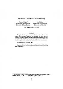
selected with reference to some absolute position. We analyze polyhedral and ellipsoidally shaped uncertainty regions and arrive at very tractable and potentially easily parallelized algorithms for solving the resulting min–max optimization problem. This model, however, does not admit dependent positional uncertainties, which can occur as a result of an accumulation of positional uncertainty as the sensor moves over the datacollection locations. Under dependent positional uncertainties, we detail a dynamic-programming (DP) formulation as a means of searching among the possible sequences of data-collection locations. This formulation also admits polyhedral and ellipsoidally shaped uncertainty regions. Although it is more computationally intensive than the case of independent errors, the results we see from the simulation are promising and point to the utility of further work involving much more tractable approximate dynamic-programming approaches. We report the results of numerical experiments involving both simulated and field data and compare these results to those of an existing technique that does not account for positional uncertainty. In all cases, we observe significant classificationperformance improvements compared to cases where sensorpositioning errors are not taken into account. The remainder of this paper is organized as follows. In Section II, we introduce the classification problem of interest and develop the positional-uncertainty framework. We consider the case of independent positional uncertainties in Section III. For dependent positional uncertainties, a dynamicprogramming formulation is presented in Section III-D. Section IV reports the results of our numerical studies for UXO characterization using electromagnetic induction (EMI) sensors. Finally, conclusions and future work are provided in Section V. II. G ENERAL P ROBLEM F ORMULATION A. Classification Based on Spatially Sampled EMI Data We consider the problem of classifying objects based on spatially sampled EMI data in the time or frequency domain. Data are assumed to be collected from a single monostatic sensor, as depicted in Fig. 1. The generalizations to multiple sets of data from multistatic-sensing systems are conceptually straightforward but notationally burdensome. It is assumed that our sensor stops to collect data at N distinct-transmitter/receiver-location combinations. We associate with the ith data-collection location the nominal coordinate r i = (xi , yi , zi ), for i = 1, . . . , N . At each location, we assume that M time or frequency samples are taken. Under this model, the kth data sample at the jth sensor location is given by [17] dj,k = gjT RT Λk Rfj + σnj,k = sj,k + σnj,k

(1) (2)

where gj is a 3 × 1 vector holding the (x, y, and z) components of the magnetic field induced at location r j by a current of I units flowing through the receive coil, and fj represents the excitation-field vector evaluated at the dipole position. Functional forms for f and g are provided in [39]. The noise variance

TAROKH AND MILLER: SUBSURFACE SENSING UNDER SENSOR POSITIONAL UNCERTAINTY

677

To show the explicit dependence of our model on both the object parameters and the positions of the sensors at each datacollection location, we express, using (2), the model for the kth data value collected at the jth location as sk (θ, r j ) = g T (θ, r j )RT (θ)Λk (θ)RT (θ)f (θ, r j )

Fig. 1. Monostatic sensor for data collection, consisting of two concentric coils for transmitting and receiving electromagnetic energy. The sensor is centered at nominal location r.

is σ and nj,k is a zero-mean unit-variance white Gaussian random variable used to represent the measurement noise. The 3 × 3 matrix R is a 3-D rotation matrix used to transform the global-coordinate frame of reference to the rotated local frame of reference at the object. Algebraically, the matrix R diagonalizes the complex-valued magnetic polarizability tensor Λk . R is parameterized by three Euler angles ψ1 , ψ2 , and ψ3 and is modeled under the x-convention [40]. Thus, it is without loss of generality that we assume Λk is a diagonal 3 × 3 complex-valued matrix. For the frequency-domain version of the problem, Λk has the form  Λ(ω) = 



λ1 (ω)

.

λ2 (ω)

B. Including Positional Uncertainty in the Model

Replacing ω by t in (3) yields the time-domain form of Λk . The quantities λ1 , λ2 , and λ3 are associated with one of each of the principle axes of the object. In other words, the diagonal elements of Λk hold the scattering characteristics of the object along each of the three principle axes for the kth frequency (time) sample. The model for these quantities is given as follows [41]: ∞ ai,l ω , pi,l + ω

i = 1, 2, 3

(4)

l=1

λi (t) = −

∞

ai,l pi,l e−pi,l t u(t),

i = 1, 2, 3

where θ is a 6-D vector that holds the coordinates of the object (x, y, and z) as well as the Euler angles (ψ1 , ψ2 , and ψ3 ). The classification approach is started by constructing a target-signature library, which will be used in the actual processing. For each target of interest, this library will hold the corresponding pole values [17]. Given the library, classification is a two-step process. First, for each target in the library, the data dj,k , j = 1, . . . , N and k = 1, . . . , M are used to estimate the unknown parameters associated with that model: poles, expansion coefficients, object location, and object orientation. Second, using these estimates, we perform the classification. The classifier used in this paper is based on the fit of the kth model in the library to the available data. This involves evaluating (6) at the estimated parameter values (poles, expansion coefficients, object location, and object orientation) for the object, obtained in the first step. As explained and demonstrated more fully in [17], this approach is likely to be of use when the signal-to-noise ratio (SNR) is relatively low. It is important to note that we only study the databased-classification method as a proof-of-concept. Other classification techniques, for example, those explored in [17], can also be applied without requiring any changes to our proposed methods. Additionally, it is often of interest to incorporate clutter rejection into the classifier. Such an extension can be easily incorporated into a classifier by adopting a thresholding technique (see, for example, [18] and references therein).

(3)

λ3 (ω)

λi (ω) =

(6)

(5)

l=1

√ where  = −1, ai,l is the expansion coefficient for the lth term corresponding to the ith axis, pi,l is the lth pole for the ith axis, and u(t) is the unit-step function. Equations (4) and (5) only hold for nonferrous objects. In the case of ferrous objects, a dc offset must be added in the frequency-domain version of the model. Correspondingly, a Dirac delta function must be included in the time-domain version of the model.

As we motivated in Section I, it is often the case that the precise sensor position at each sensor location is not known. To model this situation, the precise coordinates of the jth location r j are taken to be the sum of two components, for each j = 1, . . . , N r j = r 0,j + δr j

(7)

where r 0,j is the nominal (equivalently expected or understood) position for the jth sensor location and δr j is the perturbation to r 0,j that yields the true sensor position at the jth data-collection location. We denote the region of uncertainty within which the true ith sensor location is known to reside as Sj . The set of error tolerances to which the nominal-location information is subjected is defined for the jth location by Sj = δr = r − r 0,j : r ∈ Sj .

(8)

We assume that Sj is a connected convex and bounded region for each j = 1, . . . , N , for example, a box or an ellipsoid. This region could be a conservative estimate of the true set of error

678


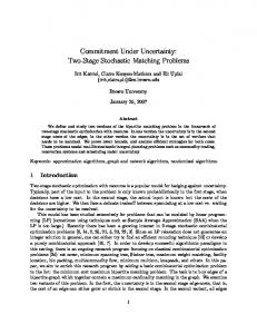
Fig. 2. Data are collected at N locations over a field of interest. Location j has associated with it a region of uncertainty Sj , shown here for every j as a boxshaped region. The dashed line connecting data-collection locations indicates the sequence in which data are collected over the field.

tolerances in measurement but reflects the best range that is known. Fig. 2 depicts the sensor locations over which data are collected. Note that the region of uncertainty is depicted at each location as a box. Fig. 2 depicts the successive sensor positions as being visited sequentially. Sequential data collection is common; modeling data collection that relies upon dead reckoning (for example, a device employing an inertial measurement unit). In such a scenario, it is the case that successive perturbation values are dependent, since each successive location is determined nominally from the last location, but there is some uncertainty in the calculation of the new position. Given the manner in which data are collected [20], it is reasonable to assume that successive data-collection locations depend only the current sensor positions and not on past sensor positions. In probability terms, the set of sensor positions evolves in a Markovian fashion [42]. Consequently, this scenario is effectively modeled through a first-order autoregressive relationship with parameter α as follows. Suppose that nominal locations r 1 , . . . , r N are fixed values corresponding to the known but inexact sensor locations. Then, the sets S1 , . . . , SN are related according to Sj (δr j−1 ) = δr j = αδr j−1 + δr : δr ∈ Sjnew

(9)

for j = 2, . . . , N . We have explicitly shown the dependence of the jth uncertainty region on the perturbation at the (j − 1)th sensor location by defining Sj as a set-valued function. In (9), we refer to the set Sjnew as the set of innovations at the jth location. This set reflects the new positional uncertainty introduced by measurement at the jth location. In words, our model for successive uncertainty regions begins with the first uncertainty region S1 . The next uncertainty region S2 is defined in terms of an element of S1 . Hence, given that some uncertainty δr 1 was realized in the region S1 , the uncertainty value at the second sensor location δr 2 must depend on δr 1 . The actual dependence is given by δr 2 = αδr 1 + δr, where δr is the additional uncertainty (or innovation) that compounds with the initial uncertainty. This new uncertainty is restricted to the set Sjnew . The same relationship follows for subsequent sensor locations. The parameter α essentially captures the degree to which the sensor positional uncertainty of the previous data-collection location affects that of the subsequent data-collection location.

Note that when α = 0, this model specializes to the case where each perturbation term is independent of the others, which is a common scenario when a fixed reference (such as GPS) is used for calculation of each sensor location [14]. A nonzero value of α can arise under several circumstances, such as when no fixed reference is available and, consequently, error is compounded due to fluctuations or poor estimates of the velocity of the sensor as it collects data at regularly spaced intervals of time or due to miscalculations from equipment or human failure. The value α = 1 is particularly applicable to data-collection scenarios where dead reckoning with no fixed reference is available. In such a situation, the current sensor position is treated as the current nominal data-collection location when computing the subsequent data-collection location. The value of α clearly depends on the data-collection mechanism and must be modeled appropriately in order to reach the best possible optimization goals. We denote by R the set of admissible trajectories of perturbation values, (δr 1 , . . . , δr N ) under the above model (9). R may be expressed as R = {(δr 1 , . . . , δr N ) : δr 1 ∈ S1 , δr j ∈ Sj (δr j−1 ) ∀j = 2, . . . , N } . (10) The set of admissible true sensor locations is then given by R = {(r 1 ,. . . ,r N ) : r j = r 0,j +δr j

∀j, (δr 1 ,. . . ,δr N ) ∈ R} . (11)

III. M IN –M AX F ORMULATION FOR U NKNOWN B UT B OUNDED P OSITIONAL U NCERTAINTY In this section, we formulate a min–max optimization strategy for our classification problem, which is subjected to sensor positional uncertainty. Our mathematical formulation requires, first, a cost function over which to optimize. As is typical in many data inversion applications where measurement noise is modeled using a white Gaussian noise process, here, we employ a cost functional equal to the norm of the squared-error difference between the data observed and the prediction of the data provided by the model s over all θ Jˆ1 (θ, r 1 , . . . , r N ) =

N M

dj,k − sk (θ, r j ) 2 .

(12)

j=1 k=1

The problem now is how to specify the r j in function sk in Jˆ1 . Typically, the r j are set equal to their nominal values r 0,j , and an LS estimate of θ is found. Here, we seek to augment the minimum error notion of optimality in a manner that easily incorporates the additional knowledge we have concerning the geometry of the Sj for j = 1, . . . , N . Essentially, the problem we have is to determine a set of primary parameters θ in the presence of a collection of “nuisance” parameters, the r j , which are restricted to exist in known regions of space. This additional knowledge concerning the positional uncertainties may be


incorporated into our cost functional to yield the augmented cost functional Jˆ2 , given by1 Jˆ2 (θ, r 1 , . . . , r N ) =

N M

amounts to selecting that θ that minimizes the worst error, as measured by Jˆ2 (θ, r 1 , . . . , r N ) as (r 1 , . . . , r N ) ranges over ˆ our estimate of θ, is defined R for j = 1, . . . , N . Formally, θ, through the min–max formulation as ˆ = arg min θ

j=1 k=1

× dj,k − sk (θ, r j ) 2 + γ

679

N

θ

δr j − αδr j−1 2 . (13)

j=2

The cost functional in (13) penalizes simultaneously the fidelity of the data reconstruction implied by the parameter vector θ and the nearness of adjacent perturbation values, related through the coefficient α. This last term is motivated by the recursively defined model we have hypothesized for the sets Sj which implies a degree of nearness for the positional perturbations for successive data-acquisition locations. The parameter γ in (13) may be considered as a regularization coefficient that establishes the level of tradeoff between the two terms in (13). The choice of appropriate γ is a well-studied issue in the field of inverse problems. Common approaches include the L-curve and generalized cross-validation methods [43], [44]. In our case where, as we discuss below, (13) is used in the context of a dynamic-programming algorithm, it is not at all clear that such regularization-parameter-selection methods would be applicable or appropriate. Developing such methods, while very interesting, is well beyond the scope of the work in this paper, where our primary concern is in demonstrating a new approach to the larger problem of processing in the presence of positional uncertainty. Hence, in the examples presented in Section IV, we chose γ through trial and error. In fact, the value of γ = 1 was used for all examples and provided a quite strong performance. We note that (13) takes the form of the log-likelihood cost function that would result were we have to assume that the position errors themselves followed a first-order Gauss–Markov process with drift defined by α and driving noise variance related γ. We choose here not to use (13) as the basis for an extended-estimation problem where we jointly determine from the data values for both θ as well as all of the δr j . For the UXO problem of interest here, θ contains 13 parameters while the total number of positional parameters would be three times the number of sensor locations. Given specifically the well-known difficulties in estimating the decay rates for UXO objects [18], [36], [45], [46], the addition of this large number of nuisance parameters associated with the sensor locations would likely degrade the accuracy of these estimates quite severely. In the following sections, we detail an alternative approach to processing, in which we explicitly make use of the bound information used to construct the sets Sj . Specifically, we consider a “min–max” optimization problem based on (13), a well-known approach to problems involving auxiliary parameters whose values are not known exactly but are known to lie within a bounded region of space. This approach to the problem 1 The functional Jˆ does not show an explicit dependence on the perturbation 2 values δrj , j = 1, . . . , N , since these are given through (7), using the known nominal values r0,j and j = 1, . . . , N .

max

(r 1 ,...,r N )∈R

Jˆ2 (θ, r 1 , . . . , r N ).

(14)

From (6), it is clear that sk is nonlinear in the position values r 1 , . . . , r N . Since the fields for these sensors are very smooth relative to the spatial scales of the perturbation to the position, for sufficiently small values δr 1 , . . . , δr N , the following firstorder approximation is valid: sk (θ, r j ) = sk (θ, r 0,j ) + Ak (θ, r 0,j )δr j + o(δr j )

(15)

where we have adopted the little-o notation to represent the higher order terms in the expansion of sk (θ, r j ). Formally, if the function h(r) = o(r) then (h(r)/r) → 0 as r → 0 [47]. The quantity Ak (θ, r 0,j ) is a 1 × 3 vector, whose components, respectively, equal the partial derivative of sk with respect to xj , yj , and zj , evaluated at the respective nominal coordinates x0,j , y0,j , and z0,j . We may then apply (15) in (14) to yield a new min–max formulation with a cost functional that is quadratic in the unknown perturbations. Let J(θ, δr 1 , . . . , δr N ) =

N M

dj,k − sk (θ, r 0,j )

j=1 k=1

− Ak (θ, r 0,j )δr j 2 +γ

N

δr j − αδr j−1 2

(16)

j=2

¯ 2 d − Aδr = ¯

(17)

where the simple expression in (17) follows easily from (16) by ¯ and matrix A. ¯ Furthermore, we appropriately defining vector d have represented δr = (δr 1 , . . . , δr N ). Then, our simplified min–max formulation is given by ˆ = arg min θ θ

max

(δr 1 ,...,δr N )∈R

J(θ, δr 1 , . . . , δr N ).

(18)

Our next result allows us to conclude that the optimal value of the inner maximization in (18) is achieved on the boundary of R. Theorem 1: The vector (δr ∗1 , . . . , δr ∗N ) achieving the maximum value in max

(δr 1 ,...,δr N )∈R

J(θ, δr 1 , . . . , δr N )

(19)

lies on the boundary of R. Proof: See Appendix A. Applying Theorem 1, we can conclude that the space of feasible vectors (δr 1 , . . . , δr N ), over which the inner maximization in (18) must be taken, can be greatly reduced by searching over only the boundary of R. We may not, however, conclude that δr j lies on the boundary of Sj for j = 1, . . . , N . We shall

680


demonstrate (in Section III-A) that in the case of α = 0, this property is indeed true and results in a great simplification of the problem. For general α > 0, we will employ a dynamicprogramming algorithm to obtain the optimal inner maximization. This general formulation appears in Section III-D. A. Case of α = 0: Separable Optimization When α = 0, there is no assumed or known relationship between the adjacent perturbation values. Consequently, the penalty incorporated in the cost functional J associated with the relationship between adjacent perturbations is treated in this section as being unnecessary. We ensure this is the case by maintaining γ = 0, whenever α = 0. Thus, for α = 0, we have the following separation property: J(θ, δr 1 , . . . , δr N ) =

N M j=1 k=1

=

N

(20)

¯j − A ¯ j δrj 2

d

(21)

Jj (θ, δr j )

(22)

j=1

=

N

Blx ,ly ,lz = {δr = (δx, δy, δz) : |δx| ≤ lx , |δy| ≤ ly , |δz| ≤ lz } . (26) For the ellipsoidal region, denoted as Elx ,ly ,lz , we make use of the same parameters lx , ly , and lz to indicate each of the three axis lengths corresponding to a 3-D ellipsoid. We omit rotation angles from the characterization of the ellipsoid, although, this can be easily incorporated

δx2 δy 2 δz 2 Elx ,ly ,lz = δr = (δx, δy, δz) : 2 + 2 + 2 ≤ 1 . lx ly lz (27) B. Polyhedral Region of Uncertainty Under α = 0

dj,k − sk (θ, r0,j ) − Ak (θ, r 0,j )δr j 2

and lz , which indicate the length, width, and height of the region of uncertainty

Under α = 0, for any region of uncertainty, Theorem 2 allows us to restrict our search in the inner maximization of (24) to the boundary of the region. However, an even stronger statement can be made for the case of polyhedral regions (which include box-shaped regions), as follows. Theorem 3: Let P be any polyhedral region of uncertainty. The value δr ∗j achieving the maximum value in max Jj (θ, δr j )

where we define Jj = ΣM k=1 dj,k − sk (θ, r 0,j ) − 2 Ak (θ, r 0,j )δr j , for j = 1, . . . , N . Under this separation, our optimization (18) can be expressed as ˆ = arg min θ θ

=

N j=1

max

(δr 1 ,...,δr N )∈R

J(θ, r 1 , . . . , r N )

arg min max Jj (θ, δr j ). θ

δr j ∈Sj

(23)

max Jj (θ, δr j )

lies at one of the extreme points (a corner) of P. Proof: See Appendix B. As a result of Theorem 3, when α = 0, we need only test the extreme points of the polyhedral region of uncertainty in order to determine the overall cost-maximizing perturbation value over the entire region. For the box-shaped region, this implies a search over the eight corner points of the box.

(24) C. Ellipsoidal-Shaped Region of Uncertainty Under α = 0

Since Sj (δr j−1 ) has no dependence on δr j−1 when α = 0, we have that Sj (δr j−1 ) = Sjnew for j = 2, . . . , N . To simplify the notation, we have dropped the expression of Sj as a function of δr j−1 for j = 2, . . . , N in (24). Theorem 2: For j = 1, . . . , N , the point δr ∗j achieves the maximum value in δr j ∈Sj

(28)

δr j ∈P

j=1

We now turn our attention to the case of an ellipsoidal region of uncertainty. The inner maximization in (24) can be expressed as max

δr j ∈Elx ,ly ,lz

Jj (θ, δr j ) =

max

2 ,1/l2 ,1/l2 })δr=1 δr T diag({1/lx y z

(25)

lies on the boundary of Sj . Proof: Since Jj is convex and quadratic in δr j , the proof for each j follows identically to the proof of Theorem 1. We omit the details because of this redundancy. We now consider two special structures for the regions of uncertainty: polyhedral and ellipsoidal regions. For simplicity of exposition, we assume that each region of uncertainty is identical over the possible sensor locations, S1 = · · · = SN . We denote the polyhedral-shaped uncertainty region P. For the special case of a box-shaped region, we denote the region Blx ,ly ,lz . This region is parameterized by three values, lx , ly ,

¯j − A ¯ j δr 2 × d

(29)

 0 0 . 1/lz2

(30)

where diag

2

1/lx2 , 1/ly2 , 1/lz



1/lx2 = 0 0

0 1/ly2 0

We will approach this constrained optimization through the Lagrange multiplier method. Using Lagrange multiplier λ, we consider the unconstrained optimization

2 T 2 2 2 ¯ ¯ max dj − Aj δr +λ δr diag 1/lx , 1/ly , 1/lz δr−1 . δr

(31)


Through a simple matrix derivative, we obtain the optimality condition ¯ + 2 λ diag 1/l2 , 1/l2 , 1/l2 + A ¯ TA ¯ Td ¯ δr = 0 −2A x y z (32) which implies the optimal value δr ∗j satisfies

681

The dynamic-programming algorithm for achieving maximum cost in the inner maximization of (18) is given by V1 = max

δr∈S1

In order to characterize the value of λ such that δr ∗j T δr ∗j = 1, simple algebraic manipulation yields the following series of equations: (34) δr ∗j T diag 1/lx2 , 1/ly2 , 1/lz2 δr ∗j = diag ({1/lx , 1/ly , 1/lz }) 2 −1 ¯ ¯ TA ¯ ¯ Td × λ diag 1/lx2 , 1/ly2 , 1/lz2 + A A 2 −1 T T ˆ ˆ ˆ ¯ ¯ A ¯ ¯ d λI + A = A ¯ 2 = V (λI + ΣT Σ)−1 ΣT U d ¯ T U T Σ λI + ΣT Σ −2 ΣT U d ¯ =d 2 2 2 ˆ ˆ ˆ ¯ ¯ ¯ d d d 1 2 3 = + + . (λ + σ12 )2 (λ + σ22 )2 (λ + σ32 )2

(35) (36) (37) (38)

k=1

Vj (δr j−1 ) =

δr j ∈Sj (δr j−1 )

+ Vj+1 (δr j ),

j = 2, . . . , N

(42)

VN +1 = 0.

(43)

Since the uncertainty regions are continuous, we must discretize the set R in order to execute the DP algorithm. Our approximation will lead to a finite number of possible trajectories. We will demonstrate that our approximation is consistent, in the sense that as our discretization becomes finer; we approach the optimal maximum cost achieved in (41)–(43). Let Z be the set of integers. Define the rational lattice Ln by Ln = {r ∈ R3N : nr i ∈ Z,

for i = 1, . . . , 3N }.

(44)

Then, we define the discretized space of uncertainty trajectories Rn = Ln ∩ R.

(45)

This discretization induces regions Sjn for j = 1, . . . , n, which we define recursively as (46) S1n = δr 1 ∈ R3 : (δr 1 , δr ) ∈ Rn Sjn (δr j−1 ) = δr j ∈ R3 : (δr , δr j−1 , δr j , δr )

∈ R , δr ∈ R n

3(j−2)

,

j = 2, . . . , N. (47)

Our approximate DP algorithm, parameterized by the discretization index n, is then given for n = 1, 2, . . . , by V1n = maxn δr 1 ∈S1

M

d1,k − sk (θ, r 0,1 ) − Ak (θ, r 0,1 )

k=1

D. General Case of α > 0: Dynamic-Programming Approach In this section, we treat the general problem for α > 0. A simple dynamic-programming formulation is introduced for the optimal solution to the inner maximization in (18). Whereas the polyhedral and ellipsoidal uncertainty regions under α = 0 yield simple and tractable solution approaches to the inner maximization in (18), the general formulation for α > 0 can result in a trajectory of uncertainty values (δr 1 , . . . , δr N ), where it is not necessarily true that δr j lies on the boundary of Sj for j = 1, . . . , N .

dj,k − sk (θ, r 0,j )

k=1

−Ak (θ, r 0,j )δr j 2 + γ δr j − αδr j−1 2

2 ˆ2 ˆ2 ˆ ¯ λ+σ 2 2 λ+σ 2 2 + d ¯ λ+σ 2 2 λ+σ 2 2 + d ¯ λ+σ 2 2 d 2 3 1 3 1 1 2 3 2 2 2 2 × λ+σ22 = λ+σ12 λ+σ22 λ+σ32 . (40)

Thus, we have reduced the problem in the case of ellipsoidal regions of uncertainty to obtaining the roots of a sixth-order polynomial and testing each of the implied boundary locations for maximum cost in Jj .

(41) M

max

(39)

ˆ ¯ =A ¯ diag({lx , ly , lz }). The singular value We have defined A ¯ ¯ = U ΣV T , where U and V decomposition of A is given by A are orthogonal matrixes having orthonormal columns. We have ˆ ¯ Since we re¯ = ΣT U d. additionally defined the 3 × 1 vector d ∗T 2 2 2 quire δr j diag({1/lx , 1/ly , 1/lz })δr ∗j = 1, (34)–(39) imply that λ must satisfy the sixth-order polynomial equation

d1,k −sk (θ, r 0,1 )−Ak (θ, r 0,1 )δr 1 2

+ V2 (δr 1 )

−1 ¯ (33) ¯ TA ¯ ¯ T d. δr ∗j = λ diag 1/lx2 , 1/ly2 , 1/lz2 + A A

M

× δr 1 2 + V2n (δr 1 ) Vjn (δr j−1 ) =

max n

δr j ∈Sj (δr j−1 )

(48)

M k=1

× dj,k − sk (θ, r 0,j ) − Ak (θ, r 0,j )δr j 2 n + γ δr j − αδr j−1 2 + Vj+1 (δr j ),

j = 2, . . . , N VNn+1

= 0.

(49) (50)

682


Theorem 4: The approximation (45) is consistent, in the sense that V1n → V1 as n → ∞. Proof: Suppose the trajectory δr = (δr 1 , . . . , δr N ) ∈ R achieves the maximum cost in (41)–(43). Let ε > 0 and define Bε = δr ∈ R3N : δr − δr 2 ≤ ) . (51) By the definition of R, the set Bε ∩ R must be a convex set of nonzero volume. This implies that there must exist a rationalvalued vector δr ∈ Bε ∩ R. Let the lowest common denominator of all the components of δr be n. Then, clearly, nδr is integer-valued. Thus, δr ∈ Rn . Expressing δr n = δr + ∆r, we obtain ¯ 2 − ¯ ¯ n 2 d − Aδr d − Aδr |J(θ, δr) − J(θ, δr n )| = ¯ (52) 2 T ¯ ¯ − Aδr ¯ d ¯ − 2∆r T A = A∆r ≤ σ12 ∆r 2 ≤ σ12 ε

(53) ¯ + 2σ1 ∆r ¯ d − Aδr

√ ¯ + 2σ1 ε ¯ d − Aδr

(54) (55)

ˆ Noting where σ1 is the maximum singular value of matrix A. ¯ − Aδr ¯ that the quantity d is a constant, we have that the approximation is consistent, as desired. IV. N UMERICAL S TUDIES In this section, we validate the analysis of our previous sections through simulation studies. We consider both the cases of independent and dependent sequences of data-collection locations. A. Independent Data-Collection Locations: Simulated Data Our first numerical study makes use of simulated data to test the classification algorithm when there is no knowledge of dependence between adjacent data-collection locations. Thus, the algorithm employs the value α = 0. In this scenario, our sensing-system model is comprised of two square colocated transmit and receive coils with dimensions 0.5 m on each side. These coils sample a 1-m square area on an equally spaced 4 × 4 grid of measurement points. This models the scenario where an object has already been detected and data collection is being conducted in the vicinity of the object to assist in the classification process. Our model assumes that the object to be classified resides at a depth between 0.05 and 2.0 m below the surface of the ground. The sensor is modeled as a frequencydomain sensor, with complex data (in-phase and quadrature) collected at 30 equally logarithmically spaced frequencies between 10 and 30 kHz. Our simulated library of target objects consists of four objects: a 3 in long × 1 in diameter stainless-steel cylinder (S1), a 6 in long × 1 in diameter stainless-steel cylinder (S2), a 3 in long × 1 in diameter aluminum cylinder (A1), and

a 6 in long × 1 in diameter aluminum cylinder (A2). The “ground truth” model, for the scattering characteristics of these targets, was obtained using the method of [36], where the dipole model was taken to be exact. Four terms were kept in each λi summations in (4), and all expansion coefficients were taken to be one (see [36] for additional details). Data collection is done with the SNR set at approximately 12 dB, with noise always assumed to be independent identically normally distributed. The SNR for this and all other cases was calculated as follows: SNR = 10 log10

d 2 σ 2 ld

(56)

where d denotes the signal vector, ld is its length, and σ 2 denotes the noise variance. Throughout this paper, we assume that the noise is independent identically Gaussian distributed. We make use of the “databased” classification method of [17], which uses a classification statistic that essentially tests for a best fit to the object library. The pole characteristics of our simulated targets are the same as those in [17, Sec. IV]. As noted in [17], the pole characteristics vary significantly as a function of object material but much less so between objects of the same material. Consequently, we anticipate significantly better classification of object material than of precise object. A Monte Carlo approach was used to analyze and compare the performance of our algorithms for this library. Specifically, 100 separate runs were carried out for each object, where we randomized uniformly over object type, object location, orientation, and additive sensor noise (by selecting a new set of parameters according to a uniform distribution at each Monte Carlo run). The corresponding values of the Euler angles were chosen randomly (with a uniform distribution) over their full range of definition (either 0 to 2π or 0 to π depending on the angle [40]). Our Monte Carlo studies were used to test both the cases of box-shaped and ellipsoidal-shaped uncertainty regions, modeled in (26) and (27), respectively. In the case of box-shaped uncertainty, each uncertainty region was assumed to be 10 cm on each side, while for the ellipse-shaped uncertainty, we assumed a spherical uncertainty region of 10-cm diameter. We compared the classification results against the classification results of the pole-based classification scheme in [17], where the algorithm is agnostic with regard to sensor positional uncertainty. The classification results for the box-shaped uncertainty regions are summarized in the confusion matrixes of Tables I and II, while those of the ellipsoidal-shaped uncertainty regions are summarized in Tables III and IV. The element on the ith row and jth column of each matrix displays the number of times object i was the true target, and object j was selected by the given processing scheme. Direct comparison between Tables I and II for the box case, and of Tables III and IV for the ellipsoidal case, show dramatic improvements both in correct classification of type and material of the targets under study when positional uncertainties are taken into consideration. For the data generated under box-shaped positional uncertainty, the correct-material-classification rate improves from 25%, 39% (Aluminum targets), 63%, and 58% (Steel targets) to 95%,


683

TABLE I CLASSIFICATION RESULTS FOR BOX-SHAPED POSITIONAL UNCERTAINTY UNDER THE ALGORITHM THAT IGNORES UNCERTAINTY

TABLE II CLASSIFICATION RESULTS FOR BOX-SHAPED POSITIONAL UNCERTAINTY UNDER THE MIN–MAX FORMULATION

Fig. 3. Plot of percentage of successful classification of object type for varying bounding-box dimensions used within the optimization.

TABLE III CLASSIFICATION RESULTS FOR ELLIPSOIDAL-SHAPED POSITIONAL UNCERTAINTY UNDER THE ALGORITHM THAT IGNORES UNCERTAINTY

TABLE IV CLASSIFICATION RESULTS FOR ELLIPSOIDAL-SHAPED POSITIONAL UNCERTAINTY UNDER THE MIN–MAX FORMULATION

95%, 100%, and 100%, respectively. Similarly, the correctmaterial-classification rate in the case of data generated under ellipsoidal-shaped positional uncertainty improves from 24%, 26% (Aluminum targets), 72%, and 64% (Steel targets) to 95%, 95%, 100%, and 100%, respectively. B. Robustness of the Algorithm We consider the possibility of having incorrect knowledge of the bounding information for sensor positional uncertainty, in

order to determine the robustness of our technique. While this robustness study was only conducted for the case of α = 0, we expect similar results under nonzero values of α. We considered objects A1 and S2, detailed in Section IV-A. For each target of interest, we generated data sets in a similar fashion as described in Section IV-A. In these studies, however, we assume that the true error in sensor position is restricted in the x and y directions by 25 cm and in the z direction by 10 cm. Given each data set, we conducted optimizations assuming a range of bounding boxes. First, we considered a region equal to a point, meaning that we assume no knowledge of any uncertainty in the sensor positions. This assumption is similar to the algorithm presented in [17]. Subsequently, we considered regions with nonzero volume, having z dimension equal to 10 cm in each case, while the x and y dimensions were simultaneously stepped from 5 to 30 cm in increments of 5 cm. The results of this paper are presented in Fig. 3, where each data point represents the percentage of successful targettype classifications (on the vertical axis) corresponding to a particular bounding-box dimension (on the horizontal axis). Note that the value of 0 cm on the horizontal axis represents the case where our optimization assumed the bounding region to be equal to a point. Each data point is obtained by considering 100 independently generated data sets. As is clear from Fig. 3, the classifier behaves well for bounding boxes having dimensions in the vicinity of the true bounding box (25 cm in both the x and y directions). We thus conclude that our algorithm is robust to the presence of incorrect bounding information. C. Dependent Positional Uncertainty: Simulated Data This simulation study concerns dependent positional uncertainties, where a known or assumed value α = 0 ties each successive positional uncertainty value to its predecessor. We make use of simulated data. The sensing system and region of interest containing the target to be classified are identical to that in Section IV-A. Data are assumed to be collected over a

684


TABLE V CLASSIFICATION RESULTS FOR DEPENDENT POSITIONAL UNCERTAINTIES FOR THE MIN–MAX FORMULATION UNDER THE ASSUMPTION OF α = 0

TABLE VII GEM-3 PIPE-DATA-POLE LIBRARY

TABLE VI CLASSIFICATION RESULTS FOR DEPENDENT POSITIONAL UNCERTAINTIES FOR THE APPROXIMATE DYNAMIC-PROGRAMMING FORMULATION

square grid of 16 data-collection locations, with the sequence of locations following the winding path depicted in Fig. 2. As in Section IV-A, we assume that data are collected over 30 logarithmically spaced frequencies. We make use of the correlation parameter α = 1 and assume that each innovation region is a box-shaped region of uncertainty with each edge having 10 cm in length. Recall that the innovation region consists of the set of new positional uncertainty associated with a data-collection location that compounds with the previous location’s positional uncertainty. The simulation results for this paper are provided in the confusion matrixes of Tables V and VI: Table V contains the classification results for the min–max algorithm that assumes α = 0, which corresponds to the case of no knowledge of any correlation between adjacent uncertainty values; Table VI contains the classification results for the approximate dynamic program outlined in (48)–(50), with a sampling of the space of positional trajectories at intervals of 5 cm. Clearly, the dynamicprogramming approach provides significant performance improvements over the min–max algorithm that operates under the assumption of α = 0. Here, the correct-type classification was improved from 51%, 51%, 68%, and 69% for targets A1, A2, S1, and S2, respectively, to 91%, 87%, 93%, and 92%, respectively. D. Field-Data Studies Our second target library is comprised of nine target types whose details are shown in Table VII, where we have separated these targets into three sets, designated by letters L, M , and S. The letter L corresponds to targets that are deeply buried at a depth ranging from 90 to 110 cm. The letter M corresponds to targets buried at a depth ranging from 50 to 80 cm. Finally,

the letter S corresponds to shallowly buried targets at a depth ranging from 10 to 30 cm. This labeling is consistent with the notation of [17] and [20]. The ground truth and the measured data for this paper were obtained by the authors of [20], where the authors measured the data in a 10 × 10 m field that contained over 21 metallic targets (listed in Table VII). This test site (detailed in [20]) is located in Raleigh, NC, and was specially designed by Geophex Inc. The data for this sensing system come from the GEM-3 sensor developed by Geophex. This sensor has been used successfully in many environmental sites and can detect small targets, such as UXO and landmines, providing high spatial resolution [20]. The data were obtained using the dead-reckoning method at a line spacing of 25 cm and a height of about 20 cm above the ground. The GEM-3 sensor collected complex-valued frequency-domain data at five different frequencies, in a bandwidth from 30 Hz to 24 kHz. The GEM-3, in this case, collected about 8–10 data points per second, which resulted in a data interval of about 15 cm [20]. According to [20], the positional error for such data could be as large as 20 cm due to uneven walking speed and incorrect walking path. The error associated with sensor height can be up to 5 cm at some points [20]. These values were applied as the respective length, width, and height of the box-shaped positional uncertainty region. Since no notion of the correlation of one uncertainty region to the next was available with the data, we initially proceed with an assumption of α = 0. Classification results for the algorithm presented in [17] demonstrated reasonable performance with regard to this data, even without considering positional uncertainties. However, [17] required distinguishing between deeply and shallowly buried objects and applying appropriate classifiers (respectively, databased and pole-based classifiers). Here, we restrict our min–max formulation to databased classification and compare against the algorithm of [17], when exclusively databased classification is employed. The classification results for the field data are shown in Table VIII. It is clear from the table that our min–max formulation is significantly better than the algorithm of [17] at correctly classifying the target objects. Overall, we see 47.62% of all targets correctly classified under the algorithm of [17], while our min–max formulation achieves 71.43% correct classification.


TABLE VIII CLASSIFICATION RESULTS FOR GEM-3 DATA. HERE, “C” DENOTES A C ORRECTLY C LASSIFIED T ARGET , W HILE “M” D ENOTES A M ISCLASSIFIED T ARGET

Since the field data collected in [20] were obtained using the dead-reckoning approach, one would expect that the successive sensor positions would incur accumulated positional uncertainty. Consequently, a nonzero value of α could be used within a dynamic-programming optimization approach. Unfortunately, the data collected in [20] only have a fixed boxshaped uncertainty region associated with each data-collection location, which fits well with having parameter α = 0. The limited information regarding the dependence of uncertainty from one location to the next implies that we can, at best, guess the structure of the successive innovation regions from one sensor position to the next. Nevertheless, in order to provide an additional test of our dynamic-programming approach, we have tested several objects listed in Table VIII, assuming that the sensor positional uncertainty from one location to the next can be perturbed by no more than 5 cm. We considered objects L1, M 1, M 6, S1, and S4 within this dynamic program framework and obtained identical classification results to those of the box algorithm (presented in Table VIII).

V. C ONCLUSION In this paper, we introduced a model-based algorithm that explicitly accounts for the positional uncertainties involved

685

with data collection using EMI sensors. We utilized a forward model for the EMI sensing system that relates a small set of parameters to the observed data. Although we present this paper in the context of classifying buried objects under the assumption of EMI sensor positional uncertainty, our model applies quite generally to other sensing modalities, as well as to other inverse optimization goals. Assuming that data are collected at locations having positional uncertainty, we approached the problem by looking for model parameters that minimize the maximum mismatch to the data. This maximum was taken over all possible sensor locations, which we assumed to be bounded within some finite region of the space. For the case of independent uncertainty regions at successive data-collection locations, we analyzed general polyhedral regions and ellipsoidal regions of uncertainty and determined simple characterizations of the min–max formulation over these regions. For the case of dependent uncertainty regions, we introduced a dynamic-programming formulation for determining the optimized min–max classifier output. Our numerical studies based on simulated data point to significant benefits in applying our min–max strategies. Classification of true field data also yielded improvements over approaches that do not take positional uncertainty into account. An important avenue for future research lies in addressing the heavy computational burden of applying dynamic programming for the case of dependent positional uncertainty. There is a body of literature for approximate dynamic programming that would be effective to this end (see [48] for an introduction to approximate dynamic-programming techniques). We defer discussion of such techniques from this paper as our contribution has been to introduce dynamic programming as a useful tool for addressing the problem of positional uncertainty in our classification problem. Additionally, an important avenue for future work is in the application of our model for dependent positional uncertainty to field data. While this paper has focused on the issue of uncertain sensor positions, other forms of uncertainty also arise in the classification process. In particular, it is well understood in the classification problem we have considered here that the decay rates/resonances also exhibit uncertainties [45], [46]. This property is most relevant in the design of classifiers that process poles after they have been estimated from the data and can be helpful in designing classifiers that are more robust. More recently, Miller et al. in [45] and [46] have explored how the pole clouds can be used basically as regularizers in the estimation process. Since we have focused in this paper on developing mechanism for addressing the sensor-positionaluncertainty problem in general classification settings, we have left this particular application as an interesting area of future research. Another avenue for future research includes the extension of the classifier algorithm such that it will be able to identify clutter items as objects that are not in the library. This step is important in real-world UXO and demining problems, where there is a strong desire to correctly reject clutter items. Finally, as discussed in Section III, the automatic determination of the parameter γ remains as an avenue for future research.

686


A PPENDIX A P ROOF OF T HEOREM 1

A PPENDIX B P ROOF OF T HEOREM 3

Suppose that δr ∗ = (δr ∗1 , . . . , δr ∗N ) is interior to R, which implies that there exists ) > 0 such that

Using Theorem 2, we may, without loss of generality, assume that δr ∗j lies on the boundary of P. The proof proceeds in two parts: First, we demonstrate that if δr ∗j is interior to a face of P, then there exists a point along one of the edges of the face at which the cost is greater or equal to that at δr ∗j . Subsequently, we demonstrate that if δr ∗j lies on the edge of one of the faces of P, then there exists an extreme point at which the cost is greater or equal to that at δr ∗j . Assume that δr ∗j is interior to one of the faces of P. By the structure of Jj in (21), the direction of cost improvement at location δr ∗j is given [as in (60)] by

(δr 1 , . . . , δr N ) :

N

|δr i −

δr ∗i |

≤)

⊆ R.

(57)

i=1

We will demonstrate that there exists a point on the boundary of R having cost greater or equal to that achieved at δr ∗ . Expanding (17), we have ¯Td ¯ − 2δr T A ¯ T d + δr T A ¯ T Aδr. ¯ J(θ, δr 1 , . . . , δr N ) = d (58) The derivative of J with respect to δr is then given by dJ ¯ + 2A ¯ Td ¯ T Aδr ¯ = −2A dδr

(59)

which implies that the direction of the maximum cost improvement at the point δr ∗ is oriented toward vector

¯ ¯ Td ¯ TA ¯ j δr ∗ − A A j j j. j

(69)

Let e1 and e2 be orthonormal vectors lying in the plane containing the face of P on which δr ∗j lies. The direction of cost improvement along the plane spanned by e1 and e2 is obtained through a simple projection and equals

(60)

∗ T ¯T¯ ∗ ¯T¯ ¯ T¯ ¯ T¯ δr = eT 1 Aj Aj δr j − Aj dj e1 +e2 Aj Aj δr j − Aj dj e2 . (70)

Since δr ∗ is interior to R and because R is assumed to be compact, there must exist a positive real number κ such that for any ) ∈ (0, κ]

We must consider two cases. First, if δr = 0, then let κ > 0 be the maximum real number such that δr ∗ + κe1 ∈ P. Then

¯ + 2A ¯ T Aδr ¯ Td ¯ ∗. −2A

¯ ∈R ¯ ∗−A ¯ T Aδr ¯ T d) δr ∗ + )(A

(61)

and such that there exists ) > 0 and such that for ) ∈ (0, ) ] ¯ ∈ ¯ ∗−A ¯ T Aδr ¯ Td δr ∗ + (κ + )) A / R. (62) We consider the boundary point of R, given by ¯ . ¯ Td ¯ ∗−A ¯ T Aδr δr = δr ∗ + κ A

(63)

The cost at δr satisfies the following series of relations: 2 ¯ ¯ ¯ ¯ T Aδr ¯ Td ¯ ∗ − κA − A δr ∗ + κA J(θ, δr) = d (64) 2 ¯ − Aδr ¯A ¯T d ¯ ∗ = I + κA (65) ¯ − Aδr ¯ ∗ T I + 2κA ¯A ¯ T + κ2 A ¯A ¯ TA ¯A ¯T = d ¯ − Aδr ¯ ∗) × (d

(66)

¯ − Aδr ¯ − Aδr ¯ ∗ )T (d ¯ ∗) ≥ (d

(67)

= J(θ, δr ∗ ).

(68)

The inequality relation in (67) follows from (66), because ¯A ¯ T and A ¯A ¯ TA ¯A ¯ T must each be positive the matrixes κA semidefinite. Thus, these matrixes can only contribute positive cost to J(θ, δr ). From (68), we have that the boundary point δr of R achieves greater or equal cost to the interior point δr ∗ .

¯ j δr ∗ 2 − 2κeT dj − A Jj (θ, δr ∗j + κe1 ) = ¯ j 1 T T ∗ ¯ ¯ ¯ ¯T ¯ ¯ d +κ2 eT × A j j − Aj Aj δr 1 Aj Aj e1 ¯ j δr ∗ 2 + κ2 eT A ¯ TA ¯ j e1 = ¯ dj − A j j 1 ¯ j δr ∗ 2 ≥ ¯ dj − A j ∗

= Jj (θ, δr ).

(71) (72) (73) (74)

Above, (72) follows since δr = 0, which implies e1 is or∗ ¯ ¯ Td ¯T¯ thogonal to (A j j − Aj Aj δr ). Thus, (74) implies that there exists a point on the edge of the face achieving equal or better cost than at δr ∗ . For the second case, suppose that ∆r = 0. In this case, let κ > 0 be the maximum real number such that δr ∗ + κδr ∈ P. Then ¯ j e1 eT A ¯ j e2 eT A ¯ T +2κA ¯T Jj (θ, δr ∗ +κδr) = I +2κA j j 1 2 ¯j −A ¯ j δr ∗ 2 × d j ¯j −A ¯ j δr ∗ 2 = (I +Q) d j ¯j − A ¯ j δr ∗ T (I +2Q+QQ) = d j ¯j −A ¯ j δr ∗ × d j ¯ j δr ∗ 2 ≥ ¯ dj − A j ∗

= Jj (θ, δr ).

(75) (76)

(77) (78) (79)


Above, (76) introduces the symmetric positive semidefinite ma¯ j e1 eT A ¯ j e2 eT A ¯ T + 2κA ¯ T . Then, (76) follows trix Q = 2κA j j 1 2 because Q and QQ are positive semidefinite. From (78), we have that the cost at point δr ∗ + κδr, which resides on the edge of the face, equal or greater to that at δr ∗ . Thus, we can now conclude that there is always a point on the edge of the face in which r ∗ resides, at which the cost is equal or greater to that at r ∗ . The second part of the proof deals with δr ∗ on an edge of a face of P. In this case, we assume that vector e3 is parallel to the line spanning the edge. Proceeding in a manner similar to the above analysis for a face, we can show that there is an extreme point at which the cost is greater or equal to that at δr ∗ . We omit the details of this part of the proof because of its redundancy. ACKNOWLEDGMENT The authors would like to thank L. Carin (Duke University), as well as I. J. Won and H. Huang (Geophex Ltd.) for providing us with the data used in this paper. They would also like to thank the reviewers for their comments and suggestions, which have let to significant improvement in the quality of this paper. R EFERENCES [1] B. Barrow and H. H. Nelson, “Model-based characterization of electromagnetic induction signatures obtained with the MTADS electromagnetic array,” IEEE Trans. Geosci. Remote Sens., vol. 39, no. 6, pp. 1279–1285, Jun. 2001. [2] T. H. Bell, B. J. Barrow, and J. T. Miller, “Subsurface discrimination using electromagnetic induction sensors,” IEEE Trans. Geosci. Remote Sens., vol. 39, no. 6, pp. 1286–1293, Jun. 2001. [3] L. H. Carin, Y. Yu, A. R. Dalichaouch, A. R. Perry, P. V. Czipott, and C. Baum, “On the wideband EMI response of rotationally symmetric permeable and conducting target,” IEEE Trans. Geosci. Remote Sens., vol. 39, no. 6, pp. 1206–1213, Jun. 2001. [4] R. Chesney, Y. Das, J. E. McFee, and M. Ito, “Identification of metallic spheroids by classification of their electromagnetic responses,” IEEE Trans. Pattern Anal. Mach. Intell., vol. PAMI-6, no. 6, pp. 809–820, 1984. [5] L. Collins, P. Gao, and L. Carin, “An improved Bayesian decision theoretic approach for landmine detection,” IEEE Trans. Geosci. Remote Sens., vol. 38, no. 3, pp. 1352–1361, 2000. [6] S. J. Norton and I. J. Won, “Identification of buried unexploded ordinance from broadband electromagnetic induction data,” IEEE Trans. Geosci. Remote Sens., vol. 39, no. 10, pp. 2253–2261, Oct. 2001. [7] T. H. Bell, B. Barrow, and N. Khadr, “Shape-based classification and discrimination of subsurface objects using electromagnetic induction,” in Proc. Int. Geosci. Remote Sens. Symp., 1998, pp. 509–513. [8] L. S. Riggs, J. E. Mooney, and D. E. Lawrence, “Identification of metallic mine-like objects using low frequency magnetic fields,” IEEE Trans. Geosci. Remote Sens., vol. 39, no. 1, pp. 56–66, Jan. 2001. [9] S. L. Tantum and L. M. Collins, “A comparison of algorithms for subsurface target detection and identification using time domain electromagnetic induction data,” IEEE Trans. Geosci. Remote Sens., vol. 39, no. 6, pp. 1299–1306, Jun. 2001. [10] H. Nelson and J. R. McDonald, “Multisensor towed array detection system for UXO detection,” IEEE Trans. Geosci. Remote Sens., vol. 39, no. 6, pp. 1139–1145, Jun. 2001. [11] K. Sun, K. O’Neill, F. Shubitidze, I. Shamatava, and K. D. Paulsen, “Fast data-derived fundamental spheroidal excitation models with application to UXO discrimination,” IEEE Trans. Geosci. Remote Sens., vol. 43, no. 11, pp. 2573–2583, Nov. 2005. [12] L. M. Collins, Y. Zhang, J. Li, H. Wang, L. Carin, S. Hart, S. RosePehrsson, H. Nelson, and J. McDonald, “On the low-frequency natural response of conducting and permeable targets,” IEEE Trans. Geosci. Remote Sens., vol. 37, no. 1, pp. 347–359, Jan. 1999.

687

[13] S. L. Tantum, Y. Q. Wang, and L. M. Collins, “Statistical and adaptive signal processing for UXO discrimination for next-generation sensor data,” in Proc. Prog. Electromagn. Res. Symp., 2006, p. 362. [14] S. L. Tantum, Y. Yu, Q. Zhu, Y. Q. Wang, and L. M. Collins, “Mitigating measurement position uncertainty to improve UXO detection,” in Proc. UXO Forum, 2006. [15] Y. Yu, S. L. Tantum, and L. M. Collins, “Bayesian mitigation of sensor position errors to improve unexploded ordnance detection,” IEEE Trans. Geosci. Remote Sens., submitted for publication June 19, 2006 to IEEE Geoscience and Remote Sensing Letters. [16] J. T. Smith and H. F. Morrison“Optimizing receiver configurations for resolution of equivalent dipole polarizabilities in situ,” IEEE Trans. Geosci. Remote Sens., vol. 43, no. 7, pp. 1490–1498, Jul. 2005. [17] A. B. Tarokh, E. L. Miller, I. J. Won, and H. Huang, “Statistical classification of buried objects from spatially sampled time or frequency domain EMI data,” Radio Sci., vol. 39, no. 4, pp. RS4S05.1–RS4S05.11, 2004. [18] E. L. Miller, “On some options for statistical classification of buried objects from spatially sampled time or frequency domain EMI data,” in Proc. SPIE—Conf. Detect. Mines and Mine Like Targets: VI, Apr. 2001, pp. 97–107. [19] D. Butler, “Report on a workshop on electromagnetic induction methods for UXO detection and discrimination,” Lead. Edge, vol. 23, no. 8, pp. 766–770, Aug. 2004. [20] H. Huang and I. J. Won, “Characterization of UXO-like targets using broadband electromagnetic induction sensors,” IEEE Trans. Geosci. Remote Sens., vol. 41, no. 3, pp. 652–663, Mar. 2003. [21] S. Chandrasekaran, G. H. Golub, M. Gu, and A. H. Sayed, “Parameter estimation in the presence of bounded modeling errors,” IEEE Signal Process. Lett., vol. 4, no. 7, pp. 195–197, Jul. 1997. [22] J. Garnett, Bounded Analytic Functions. New York: Springer-Verlag, 2006. [23] G. H. Golub and C. F. Van Loan, “An analysis of the total least squares problem,” SIAM J. Numer. Anal., vol. 17, no. 6, pp. 883–893, 1980. [24] A. E. Hoerl and R. W. Kennard, “Ridge regression: Biased estimation for non-orthogonal problems,” Technometrics, vol. 12, no. 1, pp. 55–67, Feb. 1970. [25] B. Hassibi, A. H. Sayed, and T. Kailath, “Recursive linear estimation in Krein spaces—Part I: Theory,” IEEE Trans. Autom. Control, vol. 41, no. 1, pp. 18–33, Jan. 1996. [26] ——, Indefinite Quadratic Estimation and Control: A Unified Approach to H2 and H ∞ Theories. Philadelphia, PA: SIAM, 1999. [27] S. V. Huffel and J. Vandewalle, The Total Least Squares Problem: Computational Aspects and Analysis. Philadelphia, PA: SIAM, 1991. [28] P. Khargonekar and K. M. Nagpal, “Filtering and smoothing in an H ∞ -setting,” IEEE Trans. Autom. Control, vol. 36, no. 2, pp. 152–166, Feb. 1991. [29] C. L. Lawson and R. J. Hanson, Solving Least-Squares Problems. Philadelphia, PA: SIAM, 1995. [30] A. H. Sayed and S. Chandrasekaran, “Parameter estimation with multiple sources and levels of uncertainties,” IEEE Trans. Signal Process., vol. 48, no. 3, pp. 680–692, Mar. 2000. [31] A. H. Sayed, B. Hassibi, and T. Kailath, “Fundamental inertia conditions for minimization of quadratic forms in indefinite metric spaces,” in Oper. Theory Adv. Appl., vol. 87. Basel, Switzerland: Birkhauser, 1996, pp. 309–347. [32] U. Shaked and Y. Theodor, “H ∞ -optimal estimation: A tutorial,” in Proc. IEEE Conf. Decis. and Control, Dec. 1992, pp. 2278–2286. [33] M. Byrtek, F. O’Sullivan, M. Muzi, and A. Spence, “An adaptation of ridge regression for improved estimation of kinetic model parameters from pet studies,” IEEE Trans. Nucl. Sci., vol. 52, no. 1, pp. 63–68, Feb. 2005. [34] R. J. Kelly, “Reducing geometric dilution of precision using ridge regression,” IEEE Trans. Aerosp. Electron. Syst., vol. 26, no. 1, pp. 154–168, Jan. 1990. [35] H. L. V. Trees, Detection, Estimation, and Modulation Theory, Part I. New York: Wiley-Interscience, 2001. [36] P. Gao, L. Collins, P. M. Garber, N. Geng, and L. Carin, “Classification of landmine-like metal targets using wideband electromagnetic induction,” IEEE Trans. Geosci. Remote Sens., vol. 38, no. 3, pp. 1352–1361, May 2000. [37] P. Gao and L. Collins, “A comparison of optimal and suboptimal processors for classification of buried metal objects,” IEEE Signal Process. Lett., vol. 6, no. 8, pp. 216–218, Aug. 1999. [38] ——, “A theoretical performance analysis and simulation of time-domain EMI sensor data for land mine detection,” IEEE Trans. Geosci. Remote Sens., vol. 38, no. 4, pp. 2042–2055, Jul. 2000.

688


[39] Y. Das, J. E. McFee, J. Toews, and G. C. Stuart, “Analysis of an electromagnetic induction detector for real-time localization of buried objects,” IEEE Trans. Geosci. Remote Sens., vol. 28, no. 3, pp. 278–287, May 1990. [40] S. Hassani, Foundations of Mathematical Physics. Boston, MA: Allyn and Bacon, 1991. [41] N. Geng, C. E. Baum, and L. Carin, “On the low-frequency natural response of conducting and permeable targets,” IEEE Trans. Geosci. Remote Sens., vol. 37, no. 1, pp. 347–359, Jan. 1999. [42] A. Leon-Garcia, Probability and Random Processes for Electrical Engineering. Reading, MA: Addison-Wesley, 1994. [43] E. L. Miller and W. C. Karl, Fundamentals of Inverse Problems, Fall 2003. Northeastern University course ECEG398 Lecture Notes. [44] P. C. Hansen, “The L-curve and its use in the numerical treatment of inverse problems,” in Computational Inverse Problems in Electrocardiology, ser. Advances in Computational Bioengineering. Southampton, U.K.: WIT Press, 2001, pp. 119–142. 5. [45] J. Stalnaker, A. Aliamiri, and E. L. Miller, “An enhanced dipole model for UXO discrimination,” in Proc. IEEE Int. Geosci. Remote Sens. Symp., Jul. 2006. [46] A. Aliamiri, J. Stalnaker, and E. L. Miller, “A Bayesian approach for classification of buried objects using non-parametric prior model,” in Proc. IEEE Int. Geosci. Remote Sens. Symp., Jul. 2006, pp. 3911–3915. [47] G. Etgen, Salas and Hille’s Calculus. Hoboken, NJ: Wiley, 1995. [48] D. Bertsekas, Dynamic Programming and Optimal Control. Belmont, MA: Athena Scientific, 2005.

Ashley B. Tarokh (S’00–M’06) received the B.S. degree in electrical engineering from Fairleigh Dickinson University, Teaneck-Hackensack, NJ, in 2000 and the M.S. and Ph.D. degrees in electrical engineering from Northeastern University, Boston, MA, in 2003 and 2005, respectively. She is currently a Postdoctoral Research Fellow in the Department of Radiology, Brigham and Women’s Hospital, Harvard Medical School. Her research is focused on developing advanced signal-processing techniques for biomedical-imaging applications. Her research interests include biomedical signal processing, bioinformatics, signal/image processing (particularly, geophysical signal processing and tomographic imaging), and digital-communication theory.

Eric L. Miller (S’90–M’95–SM’03) received the S.B., S.M., and Ph.D. degrees from the Massachusetts Institute of Technology, Cambridge, in 1990, 1992, and 1994, respectively, all in electrical engineering and computer science. He is currently a Professor with the Department of Electrical and Computer Engineering, Tufts University, Medford, MA. His research interests include physics-based tomographic-image formation and object characterization, inverse problems, in general, and inverse scattering, in particular, regularization, statistical signal and imaging processing, and computational physical modeling. This work has been carried out in the context of applications including medical imaging, nondestructive evaluation, environmental monitoring and remediation, landmine and unexploded-ordnance remediation, and automatic target detection and classification. Dr. Miller is the recipient of the CAREER Award from the National Science Foundation, in 1996, and the Outstanding Research Award from the College of Engineering at Northeastern University, in 2002. He is currently serving as an Associate Editor for the IEEE TRANSACTIONS ON GEOSCIENCE AND REMOTE SENSING and was in the same position at the IEEE TRANSACTIONS ON I MAGE P ROCESSING from 1998 to 2002. He is the Cogeneral Chair of the 2008 IEEE International Geoscience and Remote Sensing Symposium to be held in Boston, MA. He is a member of Tau Beta Pi, Phi Beta Kappa, and Eta Kappa Nu.