and Gapeyev, Levin and Pierce [9,17]. ..... Ïi; Ïi ) â R âiâ1..n and (â; Ïji ; Ïji ) â R âjiâ1..ni âiâ1..n }. We can ..... In Loren Meissner, editor, Proc. of the 1999.
Subtyping First-Class Polymorphic Components Jo˜ ao Costa Seco and Lu´ıs Caires Departamento de Inform´ atica Universidade Nova de Lisboa {Joao.Seco, Luis.Caires}@di.fct.unl.pt
Abstract. We present a statically typed, class-based object oriented language where classes are first class polymorphic values. A main contribution of this work is the design of a type system that combines first class polymorphic values with structural equirecursive types and admits a subtyping algorithm which is arguably much simpler than existing alternatives. Our development is modular and can be easily instantiated for either a Kernel-Fun or a F≤> style of subtyping discipline.
1
Introduction
When one considers the essence of programming languages and especially of programming languages with subtyping and equirecursive types the language that comes to mind is F≤ , the extension with subtypes of the polymorphic lambda calculus introduced in [7]. When object-oriented programming is at stake, languages like the object calculus of Abadi and Cardelli [1] and Momi [15] are good examples of how to express object-oriented mechanisms. However, the subtyping relations they use to relate classes, objects and mixins stays far behind the flexible relation of F≤ ; both use invariant width subtyping relations and limited recursive subtyping relations. This expressiveness gap is due to unsoundness problems when coding the self reference as a generic value parameter of methods. In FJ [13], for instance, structural equivalence of types is traded by name-based equivalence, which is convenient to overcome problems with the subtyping of recursive types. In fact, structural equivalence of types, although adopted in some experimental programming languages such as OCaml and Modula3, does not seem to have had substantial impact in main-stream object-oriented languages. Nevertheless, the increasing use of dynamic loading, late binding and mobile code in general purpose programming frameworks raises the issue of finding more flexible compatibility criteria between components. One reason is that namebased extension and subtyping as it is implemented by modern object oriented languages creates a rigid hierarchy of classes and interfaces based on their names. This implies the usage of global name spaces and, for instance, disallows the compatibility of two classes that separately combine the same set of interfaces. This problem can of course be diminished by explicitly using wrapper objects that redirect method calls and therefore make compatible two otherwise incompatible classes. But, structural equivalence would be the most natural solution to this kind of problems.
In previous work we have presented an object oriented component calculus that uses structural equivalence of types [18,19]. The calculus was ported into an experimental language that is compiled to run on the Java framework, which inherits the structural character of calculus’ type relations up to a certain level. In this paper, we extract the essential aspects of the type system of the component calculus into a core class-based language that manipulates classes as values and uses second-order equirecursive types. One of the main contributions of this paper is the presentation of a subtyping algorithm for second-order equirecursive types. Our approach is intuitive and technically much simpler to define and prove correct than previous results, such as [5]. It builds on the coinductive formulation of first-order type systems with equirecursive types of Amadio and Cardelli [2], Brandt and Henglein [3], and Gapeyev, Levin and Pierce [9,17]. The simplicity of the algorithm is directly related to the nature of the elements the algorithm manipulates which are complete judgments instead of pairs of types and to the termination conditions of the coinductive algorithm, which uses permutation-based techniques. Moreover, our development is modular, in the sense that it can be adapted to either a Kernel-Fun or a F≤> subtyping discipline. A further contribution is of this paper is the proposal of a simple composition mechanism for classes that combines the usage of structural equivalence of classes and objects with class extension mechanisms. The remainder of the paper is structured as follows: section 2 describes the class-based language and illustrates it using a small programming example; in section 3 we define a type system for the language including the subtyping relation and its properties; in section 4 we describe the algorithm that checks the type of a language expression and enunciate its properties. Finally, in section 5 we propose a new composition mechanism for extending classes that is sound under structural subtyping of classes and objects.
2
The programming language
In this section, we define a core class-based programming language whose values are classes and objects. Both objects and classes are runtime entities in our language, the main goal is to study a type system for generic components (as classes) and objects, where the polymorphic types of classes and equirecursive types of objects are related structurally. We first introduce its syntax, which is depicted in Fig. 1. It includes constructs for objects, classes, instantiation of objects, method calls, local declarations, and recursion. Class expression combines bounded type abstraction, and value abstraction over a name denoting the object self. All other constructions are interpreted as shown in Fig. 2. The evaluation relation of the language is defined by a big step semantics e ⇓ v. Among these rules the evaluation of a new e expression deserves further explanation: it relies on the evaluation of the subexpression e into a class value, and closure under recursion of self . All other rules evaluate the corresponding
Terms
Types τ :: = | | |
(variable) (variable) e :: = x | v (value) (class) | new e[τi i∈1..n ] (instantiation) (interface) (top) | e.m(ei i∈1..n ) (method call) | let x = e in e (declaration) ji ∈1..ni ) : τi i∈1..n } (interface) | rec(x : τ ) e (recursion) (recursion)
X Class[Xi ≤ τi I Top
I :: = {mi (τji | µX.I
i∈1..n
]I
Values v :: = { mi (xji : τji | class[Xi ≤ τi
ji ∈1..ni i∈1..n
) : τi = ei ](s) e
i∈1..n
} (objects) (classes)
Fig. 1. Types and terms
v ⇓ v (Value)
�
e1 ⇓ v1 e2 [x ← v1 ] ⇓ v2 (Let) let x = e1 in e2 ⇓ v2
e[x ← rec(x : τ ) e] ⇓ v (Fix) rec(x : τ ) e ⇓ v
o = {mi (xji : τji ji ∈1..ni ) : τi = ei i∈1..n } I = {m(xji : τji ji ∈1..ni ) : τi i∈1..n }
�
e ⇓ class[Xi ≤ δi i∈1..n ](s) o rec(s : I) o ⇓ v (New) new e[τi i∈1..n ] ⇓ v e ⇓ { . . . , m(xi : τi i∈1..n ) : τ = eb , . . . } e0i ⇓ vi ∀i∈1..n eb [xi ← vi i∈1..n ] ⇓ v (Call) e.m(e0i i∈1..n ) ⇓ v
Fig. 2. Big step operational semantic rules
expressions as expected. Note that classes and objects are values and hence evaluate to themselves by means of the rule (Value). Types already appear in the syntax of expressions, are are also defined in Fig. 1. We distinguish between two kinds of types: interface types and class types. Type variables range over types of any kind. A class type Class[X ≤ τ ] σ is a polymorphic type corresponding to a F≤ bounded type quantification (cf., ∀X≤τ .σ), but for convenience generalized to a list of type parameters. Interface types can be defined recursively, using type recursion µX.I; our separation of types in two categories τ and I is not essential, and only reflects the intended type usage of the object-oriented language. We illustrate our language with a very simple example that uses polymorphic memory cells. Let C be the type defined as Class[X] µY.{set(X) : Y, get() : X}, and cell some class value of type C, and consider
φ ` � (E-φ)
∆ ` τ ok (E-Var) ∆, x : τ ` �
∆`� (O-TVar) ∆ ` X ok ∆, Xj ≤ τj
j∈1..i−1
∆ ` τ ok (E-TVar) ∆, X ≤ τ ` �
∆, X ≤ Top ` I ok (O-Recursive) ∆ ` µX.I ok
` τi ok ∀i∈1..n ∆, Xi ≤ τi ∆ ` Class[Xi ≤ τi i∈1..n ] I ok
i∈1..n
` I ok
(O-Polymorphic)
∆ ` τji ok ∀ji ∈1..ni ∀i∈1..n ∆ ` τi ok ∀i∈1..n (O-Interface) ∆ ` {mi (τji ji ∈1..ni ) : τi i∈1..n } ok
Fig. 3. Well-formed types and environments
let d = class[Y](s){ test(c:C, v:Y):Y = let o1 = (new c[Y]) in let o2 = o1.set(v) in o2.get() } in let n = (new d[int]).test(cell,1) Class d defines a method test that accepts two arguments: a class value (a component) implementing memory cells c and another appropriate value v. The method instantiates the memory cell class, stores the value v in the resulting cell object, and finally retrieves the cell contents and returns it.
3
Type system
In this section we define the type system for our language. The type system has two parts, a typing system for the language expressions, and a subtyping system expressing the intended subsumption relation on types. Our presentation will focus on the latter, concentrating on the development of our approach to polymorphic recursive subtyping. 3.1
Typing Expressions
The typing of the expressions is given by the set of rules in Fig. 4, that proves judgements of the form ∆ ` e : τ , where ∆ is the typing environment declaring the types of the free value and type variables relevant for the expression e, and τ is a type. Well-formed types and environments are also defined in Fig. 3, by the judgement forms ∆ ` � and ∆ ` τ ok, as expected. Most rules follow the usual pattern, we will discuss just the particularities of our presentation. Although the abstract syntax in Fig. 1 is somewhat more liberal, notice that rule (T-Class) enforces that only record expressions are accepted as a class body, consistently with our interpretation of polymorphic types
x:τ ∈∆ (T-Var) ∆`x:τ �
∆ ` e : τ0 ∆ ` τ0 ≤ τ (T-Sub) ∆`e:τ
c = {mi (xji : τji ji ∈1..ni ) : τi = ei I = {mi (τji ji ∈1..ni ) : τi i∈1..n }
i∈1..n
∆, x : τ ` e : τ (T-Fix) ∆ ` rec(x : τ ) e : τ }
�
∆, Xj ≤ δj j∈1..m , xji : τji ji ∈1..ni , s : I ` ei : τi ∀i∈1..n (T-Class) ∆ ` class[Xj ≤ δj j∈1..m ](s) c : Class[Xj ≤ δj j∈1..m ] I ( I = {mi (τji ji ∈1..ni ) : τi i∈1..n } ) ∆, xji : τji ji ∈1..ni ` ei : τi ∀i∈1..n (T-Object) ∆ ` { mi (xji : τji ji ∈1..ni ) : τi = ei i∈1..n } : I ∆ ` e : Class[Xi ≤ δi i∈1..n ] I ∆ ` τi ≤ δi [Xj ← τj j∈1..i−1 ] ∀i∈1..n (T-New) ∆ ` new e[τi i∈1..n ] : I[Xi ← τi i∈1..n ] ∆ ` e : {. . . , m(τi i∈1..n ) : τ, . . .} ∆ ` ei : τi ∀i∈1..n (T-Call) ∆ ` e.m(ei i∈1..n ) : τ
∆ ` e1 : τ ∆, x : τ ` e2 : τ 0 (T-Let) ∆ ` let x = e1 in e2 : τ 0
Fig. 4. Typing rules
as polymorphic object-generating classes. The name s, whose scope is the class body, typed with the type of the instances of the class, is our notation for self. In the rule (T-New), the instantiation expression new is typed with a type constructed from the type declarations present in the class expression, given the proper type substitution of the type parameters, and provided that the compatibility of the type arguments with respect to the variable bounds holds. 3.2
Subtyping
Some approaches to the problem of defining a first-order subtyping relation between recursive types exist for quite a while [2,3,17]. Intuitively, the intended subsumption relation between recursive types corresponds to the usual inclusion of infinite (regular) trees, the difficulty in the polymorphic case arises due to the presence of binding occurrences of type variables on types, due to presence of type quantifiers. Usually, even for recursive types, subtyping relations have been expressed by means of inductive proof systems, where the coinduction principle appears embedded in various explicit ways [2,3]. Apart from these, the main proof rules we might expect for such a subtyping system are the ones depicted in Fig. 5. These include the usual relationships: maximality of Top, reflexivity, transitivity, width and depth record subtyping, and unfolding of recursive types. For comparing polymorphic types, we adopt a Kernel-Fun style rule, since the more general F≤ style subtyping is known to be undecidable even in the absence of recursion [16]. In any case, our approach applies equally well to Kernel-Fun and to variants such as F≤> .
∆ ` τ ≤ Top
∆`τ ≤τ
∆`τ ≤σ X≤τ ∈∆ ∆`X≤σ
∆, Xi ≤ δi i∈1..n ` I ≤ I 0 ∆ ` Class[Xi ≤ δi i∈1..n ] I ≤ Class[Xi ≤ δi
i∈1..n ]
I0
n0 ≤ n ∆ ` τi ≤ τi0 ∀i∈1..n0 ∆ ` τj0i ≤ τji ∀ji ∈1..ni ∀i∈1..n0 ∆ ` {mi (τji ji ∈1..ni ) : τi i∈1..n } ≤ {mi (τj0i ji ∈1..ni ) : τi0 i∈1..n0 } ∆ ` I ≤ J[α ← µα.J] ∆ ` I ≤ µα.J
∆ ` I[α ← µα.I] ≤ J ∆ ` µα.I ≤ J
Fig. 5. Subtyping inductive rules
Unfortunately, the adoption of these rules results in an incomplete type system, that does not seem to easily lead to a terminating algorithm, as remarked in [11], although a rather complex subtyping algorithm following this approach was already developed in [5]. In fact, our difficulties in getting a clear understanding of this work lead us to attempt a different approach, leading to the presentation in this paper. We then follow essentially the development of [9] for first-order types, and extend it in a natural way to polymorphic types. Therefore, we start from a coinductive definition of the subtyping relation, presented below. Let D denote the set of all well-formed environments and T the set of all well-formed types. We also denote by J the set D × T × T of all subtyping judgements (represented as tuples). Definition 3.1. The subtyping generating function is the mapping S ∈ P(J ) → P(J ) defined by: S(R) = {(∆; τ ; τ ) | τ ∈ T and F V (τ ) ⊆ Dom(∆)} ∪ {(∆; τ ; Top) | τ ∈ T and F V (τ ) ⊆ Dom(∆)} ∪ {(∆; X; σ) | (∆; τ ; σ) ∈ R and X ≤ τ ∈ ∆} ∪ {(∆; Class[Xi ≤ δi i∈1..n ] I; Class[Xi ≤ δi i∈1..n ] I 0 ) | (∆, Xj ≤ δj j∈1..n ; I; I 0 ) ∈ R} ∪ {(∆; I; µX.J) | (∆; I; J[X ← µX.J]) ∈ R } ∪ {(∆; µX.I; J) | (∆; I[X ← µX.I]; J) ∈ R and J 6≡ µX.J 0 } 0 0 ∪ {(∆; {mi (τji ji ∈1..ni ) : τi i∈1..n }; {mi (τj0i ji ∈1..ni ) : τi0 i∈1..n }) | n0 ≤ n and n0i = ni ∀i∈1..n0 and (∆; τi ; τi0 ) ∈ R ∀i∈1..n0 and (∆; τj0i ; τji ) ∈ R ∀ji ∈1..ni ∀i∈1..n0 }. We can verify that the mapping S is monotonic. Therefore, there exists its greatest fixed point νS ∈ P(J ). We then define the subtyping relation as follows Definition 3.2. ∆ ` τ ≤ σ , (∆, τ, σ) ∈ νS. The relation thus defined enjoys the basic properties of weakening, substitution of type variables, equivariance, narrowing and transitivity which are essential
to prove the type safety of the language (Theorem 3.10) and the correctness of the subtyping algorithm (Theorem 4.10). In general, these kind of results are proved by somewhat involved inductions on derivations; in our setting, due to the natural definition of subtyping as a greatest fixed point, we may handle them by quite standard coinductive proof techniques. We start by considering the weakening property in νS. Proposition 3.3 (Weakening). For all typing environments ∆, ∆0 ∈ D, and types τ, σ, δ ∈ T , if ∆, ∆0 ` τ ≤ σ, X 6∈ Dom(∆, ∆0 ), and Delta ` δ ok then ∆, X ≤ δ, ∆0 ` τ ≤ σ. Proof. Consider the following set: W , {(∆, X ≤ δ, ∆0 ; τ ; σ) | (∆, ∆0 ; τ ; σ) ∈ νS and X 6∈ Dom(∆, ∆0 ) and F V (δ) ⊆ Dom(∆)}. By case analysis in the definition of S we prove W to be S-consistent, W ⊆ S(W), thus by the coinduction principle we have that W ⊆ νS. ♦ We use the same coinductive technique to prove that the substitution of type variables is sound, and that the subtyping relation is closed under name permutation. Proposition 3.4 (Substitution of type variables). For all ∆, ∆0 ∈ P(J ), and τ, σ, δ, δ 0 ∈ T , if ∆, X ≤ δ, ∆0 ` τ ≤ σ and ∆ ` δ 0 ≤ δ then we have ∆, ∆0 [X ← δ 0 ] ` τ [X ← δ 0 ] ≤ σ[X ← δ 0 ]. Proposition 3.5 (Equivariance). For all ∆ ∈ P(J ), τ, σ ∈ T , if ∆ ` τ ≤ σ then ∆[X ↔ Y ] ` τ [X ↔ Y ] ≤ σ[X ↔ Y ]. We now prove that νS is transitive by considering a combined property where transitivity is expressed together with narrowing. We start by defining narrowing of typing environments, and then closure of νS under narrowing. Definition 3.6. For all ∆, ∆0 ∈ D, we have that ∆ is narrower than ∆0 with relation to R ∈ P(J ), written ∆ vR ∆0 , where the relation vR is inductively defined by letting ∅ vR ∅ and Γ, X ≤ γ vRΓ 0 , X ≤ γ 0 if Γ vRΓ 0 and (∆, γ, γ 0 ) ∈ R. Definition 3.7. For all n ∈ N we inductively define the sets Nn as follows: N0 , νS Nn , {(∆, τ, σ) | (Γ, τ, σ) ∈ Nn−1 and ∆ vNn−1 Γ }. We then define the transitive closure of νS, and prove that νS is closed under transitivity. Instead of a more direct definition, for technical convenience we present the transitivity relation based on chains of tuples with finite length. Definition 3.8 (Extended Transitive Closure of νS). T , {(∆, α0 , αn ) | ∃n∈N .∃α0 ..αn ∈T .∀i∈0..n−1 .(∆, αi , αi+1 ) ∈ Nn }
Notice that T includes the transitive closure of νS (n = 2), and closure under narrowing (n = 1). We can then state and prove Proposition 3.9 (Transitivity). If ∆ ` τ ≤ σ and ∆ ` σ ≤ γ then ∆ ` τ ≤ γ. Proof. We show that T ⊆ S(T), using an inner induction on the number of tuples and by case analysis on the last rule used on the first tuple of a chain in T. We then conclude T ⊆ νS by the coinduction principle. ♦ An interesting fact about our proof is that it exposes the loss of transitivity elimination pointed out in Ghelli’s inductive system [11]. In the particular case of the variable transitivity, a tuple of T supported by a chain of tuples in νS is supported in S(T) by a longer chain of tuples. Which nevertheless leads to the conclusion that the tuple is in the greatest fixed point of S. 3.3
Type safety
We can now state and prove subject reduction for our class based programming language, that can then be used to show that well typed programs “don’t go wrong” along usual lines. Theorem 3.10 (Subject Reduction). If ∆ ` e : τ and e ⇓ v then ∆ ` v : τ 0 where ∆ ` τ 0 ≤ τ . Proof. By induction on the length of the typing derivations and by case analysis on the last rule used. We also use in several parts the fact that all valid subtyping judgments are supported in νS. ♦ As a result of this section we obtain declarative type and subtype systems whose implementability and decidability is far from being obvious (full detailed proofs for the results in this paper can be found in [20]). In the next section, we define and explain two simple algorithms that implement them.
4
Typing algorithm
We define a type checking algorithm for our type system, thus proving that it is decidable. The algorithm is composed by two procedures: a typing algorithm that given an environment and a typable expression returns its the minimal type, and a subtyping algorithm, that is called by the typing procedure to verify the subtyping relations. 4.1
Typing expressions
Typing of expressions is implemented by interpreting a set of rules bottom up: this defines a procedure that given a typing environment and a language expression returns a type. The new algorithmic rules are shown in Fig. 6, to these rules we must add (T-Var), (T-Let), (T-Fix), and (T-New), which are exactly
� c = {mi (xji : τji ji ∈1..ni ) : τi = ei i∈1..n } I = {mi (τji ji ∈1..ni ) : τi i∈1..n } ∆, Xj ≤ δj j∈1..m , xji : τji ji ∈1..ni , s : I `a ei : τi0 ∆ ` τi0 ≤ τi ∀i∈1..n (A-Class) ∆ `a class[Xj ≤ δj j∈1..m ](s) c : Class[Xj ≤ δj j∈1..m ] I �
∆ ` τi0 ≤ τi ∀i∈1..n ∆, xji : τji ji ∈1..ni ` ei : τi0 i∈1..n j ∈1..n i i } : {mi (τji ji ∈1..ni ) : τi ) = ei ∆ ` { mi (xji : τji
i∈1..n }
(A-Object)
∆ `a e : γ ∆ ` γ ⇑ γ 0 (τ, τi i∈1..n ) = lookup(m, γ 0 ) ∆ `a ei : τi0 ∆ ` τi0 ≤ τi ∀i∈1..n (A-Call) ∆ `a e.m(ei i∈1..n ) : τ X≤σ∈∆ ∆`σ⇑τ (X-Var) ∆`X⇑τ
τ ∈ 6 Dom(∆) (X-Default) ∆`τ ⇑τ
Fig. 6. Algorithmic typing rules
as in Fig. 4. The resulting proof system is algorithmic because in all rules the resulting types are constructed either from the expression itself or from the types resulting from typing strictly smaller subexpressions. Notice that not every rule in Fig. 4 has a corresponding rule here; the (T-Sub) rule is not used in the algorithm as it depends on an unknown type that cannot be obtained neither from the expression nor from the types of the subexpressions, we replace it by subtyping verifications in rules (A-Class), (A-Object), and (A-Call). Moreover, we use an auxiliary function lookup to find a method in an interface and the judgment ∆ ` τ ⇑ σ, defined by the rules (X-Var) and (X-Default), to access the structure of type variables. 4.2
Subtyping algorithm
We now present and prove correct our subtyping algorithm for deciding membership of a tuple t ∈ J in the greatest fixed point νS. The algorithm is defined by the recursive procedure shown in Fig. 7, and closely follows existing approaches for first-order equirecursive types [2,3,9]. Briefly, these algorithms progress by computing, given a pair of types to be checked for subsumption, a consistent set of pairs that includes it: by the coinduction principle, all the pairs in the set belong to the greatest fixed point. The consistent set is built by saturating the current approximation through backward rule application, and accumulating pairs of types, until a terminal case, corresponding to the application of an axiom, or an already visited pair is found. We naturally extend those approaches building on the generating function in Definition 3.1, by defining an algorithm that manipulates judgments instead of pairs of types; this turns out to lead to a remarkably simple way of dealing with the binding information of the type variables. Notice that environments grow as a result of comparing polymorphic types, and, due to α-equivalence, the
Subtyping(A, (∆, τ, σ)) = if (∆, τ, σ) ∈' A then A else let A0 = A ∪ {(∆, τ, σ)} in if τ ≡ σ then A else if σ ≡ Top then A else if τ ≡ X then Subtyping(A0 , (∆, ∆(X), σ)) else if τ ≡ µX.τ 0 then Subtyping(A0 , (∆, τ 0 [X ← τ ], σ)) else if τ 6≡ µX.τ 0 and σ ≡ µX.σ 0 then Subtyping(A0 , (∆, τ, σ 0 [X ← σ])) 0 else if τ ≡ {mi (τji ji ∈1..ni ) : τi i∈1..n } and σ ≡ {mi (τj0i ji ∈1..ni ) : τi0 i∈1..n } then 0 A`n` where ∀i∈1..n (Ai0 = Subtyping(Ai−1 mi−1 , (∆, τi , τi )) and i i ∀j∈1..ni Aj = Subtyping(Aj−1 , (∆, τj0i , τji ))) with A0n0 = A0 else if τ ≡ Class[Xi ≤ δi i∈1..n ] I and σ ≡ Class[Xi ≤ δi i∈1..n ] I 0 then Subtyping(A0 , (∆, Xi ≤ δi i∈1..n ; I; I 0 )) else fail
Fig. 7. Subtyping algorithm greatest fixed point νS is closed under renaming (Proposition 3.5). Moreover, in our setting, the number of tuples reachable from a given tuple are finite up to such renaming and pruning of useless variables (Lemma 4.5). Therefore, our algorithm checks for membership of a tuple in the current approximation modulo a similarity relation on tuples that includes renaming, and allows us to detect cycles at the level of similarity equivalence classes, instead of expecting the exact tuple to reappear in the sequence of calls. Definition 4.1 (Similarity). Similarity is the binary relation ' on J defined by: (∆, τ, σ) ' (∆0 , τ 0 , σ 0 ), if there are two typing environments Γ ⊆ ∆ and Γ 0 ⊆ ∆0 with Γ ` τ ok, Γ ` σ ok, and Γ 0 ` τ 0 ok, Γ 0 ` σ 0 ok, and a bijection ρ : Dom(Γ ) → Dom(Γ 0 ) such that ρ(Γ ) = Γ 0 , ρ(τ ) = τ 0 , ρ(σ) = σ 0 . In the sequel we will use the following abbreviation t ∈' A , ∃u ∈ A.t ' u, in particular in the first clause of the subtyping algorithm. Notice that similarity is decidable, it can be checked by matching the structure of the types, modulo bijective renaming of their free type variables, and recursively checking if the corresponding bounds are similar. All unused variables are discarded from the comparison as it goes through the structure of types and bounds of relevant type variables in the environments. For instance, the following two tuples are similar: (X ≤ {m(τ ):τ }, Y ≤ X; µZ.{m(X):Z}; X) ' (Z ≤ {m(τ ):τ }; µX.{m(Z):X}; Z) Notice the redundancy of Y, and that the tuples are similar with the permutation [X ↔ Z]. An important fact is that the subtyping relation νS is closed under similarity. Definition 4.2 (Closure under similarity). For any R ∈ P(J ) we define its closure under similarity, noted R∗ , as follows: R∗ , {t0 | t0 ∈ J and t ∈ R and t0 ' t}.
Lemma 4.3. νS is closed under similarity (νS ∗ = νS). Proof. By substitution of type variables (Proposition 3.4), equivariance (Proposition 3.5) and then by weakening (Proposition 3.3). ♦ We now prove the correctness and decidability of the subtyping algorithm. We first show that the algorithm terminates on all inputs. This is done by showing that the search space of the algorithm is finite in some sense. To characterize such search space we introduce the following reachability relation: Definition 4.4 (Reachability). Reachability is the binary relation on J , noted t >> t0 , inductively defined as follows: 1. (∆, τ, σ) >> (∆, τ, σ) 2. if (∆, τ, σ) >> (∆0 , X, σ 0 ) then (∆, τ, σ) >> (∆0 , ∆0 (X), σ 0 ) 3. if (∆, τ, σ) >> (∆0 , Class[Xi ≤ δi i∈1..n ] I; Class[Xi ≤ δi i∈1..n ] I 0 ) then (∆, τ, σ) >> (∆0 , Xj ≤ δj j∈1..n ; I; I 0 ) 4. if (∆, τ, σ) >> (∆0 ; I; µX.J) then (∆, τ, σ) >> (∆0 ; I; J[X ← µX.J]) 5. if (∆, τ, σ) >> (∆0 ; µX.I; J) then (∆, τ, σ) >> (∆0 ; I[X ← µX.I]; J) 0 0 6. if (∆, τ, σ) >> (∆0 ; {mi (τji ji ∈1..ni ) : τi i∈1..n }; {mi (τj0i ji ∈1..ni ) : τi0 i∈1..n }) then (∆, τ, σ) >> (∆0 ; τi ; τi0 ) ∀i∈1..n0 and (∆, τ, σ) >> (∆0 ; τj0i ; τji ) ∀ji ∈1..ni ∀i∈1..n0 We let Reach(t) , {t0 | t >> t0 }. We have the following Lemma 4.5. Reach(t)/' is finite. Proof. We prove by induction on the reachability relation that all types occurring in reachable tuples are subexpressions of the initial tuple and that the number of relevant type variables in those tuples, both in the environments and in the type expressions, decreases with relation to the initial tuple. We then prove by contradiction that these two results support the fact that the set of reachable tuples, Reach(t), is finite modulo similarity. ♦ It is important to remark that the finite reachability property of Lemma 4.5 holds both for Kernel-Fun and F≤> style subtyping, although in the first case the proof is slightly more involved (see [20]). The proof also enlightens why the same result cannot be extended to F≤ . Theorem 4.6. For all A ∈ P(J ), and t ∈ J , Subtyping(A, t) terminates. Proof. By induction using a measure that represents the number of non-visited equivalence classes of reachable tuples of t. Since the algorithm always increases the visited tuples with a tuple reachable from t, the measure decreases in all cases. Hence, the algorithm terminates. ♦ To prove that our algorithm is sound and complete, it is technically convenient to follow the approach of [9] and introduce a function gfp that allows us to characterize νS in a form both suitable for the correctness proofs and for establishing the correspondence between the algorithm and the extensional definition of the subtyping relation. Moreover, unlike the analogous notion in [9], instead of accumulating tuples, our gfp function works with ' equivalence classes.
Definition 4.7. Let gfp be the partial function P(J ) × J → P(J ) defined by: ∗
gfp(A, t) = if {t} ⊆ A then A else if support(t) is undefined then undefined else let {t1 , . . . , tn } = support(t) in ∗ let A0 = A ∪ {t} in let A1 = gfp(A0 , t1 ) in ... let An = gfp(An−1 , tn ) in An . We prove next that gfp indeed characterizes the subtyping relation. Lemma 4.8 (Correctness of gfp). For all t ∈ J , and A ∈ P(J ), 1. if gfp(∅, t) = A then t ∈ νS. 2. if gfp(∅, t) is undefined then t 6∈ νS. Proof. 1. By induction in the definition of gfp to prove the following more general property: for all A, A0 ∈ P(J ), and t ∈ J , if A∗ ⊆ A and gfp(A, t) = A0 ∗ ∗ then A ⊆ A0 , A0 ⊆ A0 , {t} ⊆ A0 , and A0 ⊆ S(A0 ) ∪ A. We then conclude by considering A = ∅. 2. Also by induction on the definition of gfp. ♦ Knowing that gfp correctly checks if any tuple belongs to the subtyping relation νS, we prove that gfp and the subtyping algorithm Subtyping are equivalent. Since the algorithm terminates on all inputs (Theorem 4.6), we can show that it is sound and complete. Lemma 4.9 (Correctness of Subtyping). For all t ∈ J , A, A0 ∈ P(J ), ∗
1. Subtyping(A, t) = A0 iff gfp(A∗ , t) = A0 . 2. Subtyping(A, t) = f ail iff gfp(A∗ , t) is undefined. Proof. By induction on the recursive calls of Subtyping.
♦
Theorem 4.10 (Correctness of Subtyping). For all ∆ ∈ D, and τ, σ ∈ T , Subtyping(∅, (∆, τ, σ)) = A iff ∆ ` τ ≤ σ Proof. It follows directly from Lemmas 4.8 and 4.9.
♦
To summarize, we conclude that the type system defined in section 3 is decidable and that our typing and subtyping algorithms are sound and complete.
5
Composition of classes
We have presented a language that treats classes as first class values but that lacks class composition operations, so that no new class values can be actually created at runtime. In this section, we discuss an interesting and possible extension of this object language so to include class manipulation mechanisms,
π = [Xi0 ← γi
i∈1..n0
I = {mi (σ π) : τi π �
Class[Xi0
π 0 = [Xi00 ← γi0
]
i∈I−J
�
i∈1..n00
, mi (σ 0 π 0 ) : τi0 π 0
i∈J
]
!
})
0 δi0 i∈1..n ]
� ∆ ` e1 : ≤ {mi (σi ) : τi i∈I } ∆ ` γi ≤ δi0 ∀i∈1..n0 � 00 ∆ ` e2 : Class[Xi00 ≤ δi00 i∈1..n ] {mi (σi0 ) : τi0 i∈J } ∆ ` γi0 ≤ δi00 ∀i∈1..n00 ∆ ` mix[Xi ≤ δi i∈1..n ](e1 [γi i∈1..n0 ] / e2 [γi0 i∈1..n00 ]) : Class[Xi ≤ δi i∈1..n ]
π = [s ← s(mi ↔m0i i∈I∩J ) ] (m0i fresh) v = {mi (σi ) : τi = ei π �
i∈I−J
class[Xi0
mix[Xi ≤
π 0 = [Xi0 ← γi
�
, mi (σi0 ) : τi0 = e0i
i∈J
i∈1..n0
][Xi00 ← γi0
, m0i (σi ) : τi = ei π �
I
i∈1..n00
i∈I∩J
]
!
}
0 δi0 i∈1..n ](s)
� e1 ⇓ ≤ {mi (σi ) : τi = ei i∈I } � 00 e2 ⇓ class[Xi00 ≤ δi00 i∈1..n ](s) {mi (σi0 ) : τi0 = e0i i∈J } δi i∈1..n ](e1 [γi i∈1..n0 ] / e2 [γi0 i∈1..n00 ]) ⇓ class[Xi ≤ δi i∈1..n ](s)
e⇓v e(m↔m0 ) ⇓ v(m ↔ m0 )
vπ 0
∆`e:τ ∆ ` e(m↔m0 ) : τ (m ↔ m0 )
Fig. 8. Typing and evaluation for mix.
similar to inheritance or mixin application. As an alternative, we propose a general mechanism of class composition which combines two classes without any of them having to be developed with extension in mind. The composition mechanism is expressed as follows: 0 00 mix[Xi ≤ δi i∈1..n ](e1 [γi i∈1..n ] / e2 [γi0 i∈1..n ]) It takes two class values, e1 and e2 , and produces a new class value, parameterized by a fresh set of type parameters, containing the methods in e1 and e2 and where name clashes are resolved in favor of e2 . This is apparent in the rules in Fig. 8 which must be added to the type and evaluation systems to extend the initial language. Notice that for a mix to be well typed e1 and e2 must denote 0 00 class values, and that the arguments γi i∈1..n and γi0 i∈1..n must be compatible with the bounds of each class value. It is well known that extending a class by simply replacing the methods of one class with methods of another easily generates type inconsistencies (e.g. see [1,6]). To avoid this, we maintain the local coherence of the subsumed class, which in this case is e1 , by means of an explicit permutation of method names, e(m↔m0 ) . This corresponds to the run-time permutation of method names between m and m0 and τ (m ↔ m0 ) has the same meaning but for type expressions. The typing and evaluation rules for this expression are also depicted in 8. So, whenever s, now replaced by s(mi ↔m0i i∈I∩J ) , is evaluated in the body of a method of e1 , the methods in s are switched back to the subsumed methods of e1 that were hidden under a different name. The evaluation of such methods and possibly of other methods using the self reference passed by a method of e1 is type preserving, and thus the core language extended with mix can be shown to enjoy a subject reduction property [20].
6
Related work and concluding remarks
It is known that the type system of F≤ is not decidable [12,16] and that its extension with recursive types is non-conservative [11]. Simpler versions were proposed but even so, not free from problems: system F≤> , proposed by Castagna and Pierce, is decidable revealed to lack the minimal typing property [4] and the approach to subtyping in Kernel Fun extended with recursive types by Colazzo and Ghelli [5] results in a fairly complex algorithm; it uses a labeling mechanism to identify cycles in derivations and stop the unfolding process. The authors show that the use of renaming of type variables results in an divergent algorithm and that this labeling technique is sound. However, the algorithm only stops unfolding a given pair of types the third time it occurs. The reasons for this fact are far from intuitive. On the contrary, our approach and algorithm are a natural extension of well known techniques for first-order types. Alan Jeffrey defines in [14] a notion of simulation for higher order types using a symbolic labeled transition systems, and uses it to define a (non decidable) subtyping relation in µF≤ , there is then some connection between his approach and the general coinductive techniques we have presented here. An efficient algorithm to unify two recursive second-order types was proposed by Gauthier and Pottier in [10]. It relies on an encoding of second-order type expressions into first-order trees, and on the application of standard first-order unification algorithms for infinite trees. We have no perspective on how this may be adapted to the subtyping problem. On the other hand, we present a subtyping algorithm for second-order systems with equirecursive types which is an uniform extension of existing work on first-order equirecursive types by Amadio and Cardelli [2], Brandt and Henglein [3]. In particular, we build on the coinductive presentations of first-order type systems with recursive types of Gapeyev, Levin, and Pierce [9,17]. Our treatment of reachability modulo a similarity relation that includes equivariance (Lemma 3.5) is inspired on notions by Gabbay and Pitts [8]. Our definition and correctness proof is, from our point of view, much simpler than the ones of the algorithms referred above. Our proofs are modular, in the sense that they can be applied to any polymorphic type system with recursive types that satisfies a certain finite reachability condition up to a notion of similarity that includes equivariance. In particular, they suggest an interesting decidable fragment of F≤ , defined by restricting the subtype rule for ∀X ≤ τ.σ types to just compare bounds with the same free type variables, we leave this topic for future work. Given these results, we develop a class based language and discuss a possible extension of it that allows combination of classes with a mixin like construct, while avoiding the unsoundness problems of subsumption and class extension often found in object calculi. We would like to thank Dario Colazzo and the reviewers for their comments on a preliminary version of this work. This work is partially supported by FCT/MCES.
References 1. Martin Abadi and Luca Cardelli. A Theory of Objects. Springer, 1996. 2. Roberto M. Amadio and Luca Cardelli. Subtyping recursive types. ACM Transactions on Programming Languages and Systems, 15(4):575–631, 1993. 3. Michael Brandt and Fritz Henglein. Coinductive axiomatization of recursive type equality and subtyping. In Roger Hindley, editor, Proc. 3d Int’l Conf. on Typed Lambda Calculi and Applications (TLCA), Nancy, France, April 2–4, 1997, volume 1210, pages 63–81. Springer-Verlag, 1997. 4. Giuseppe Castagna and Benjamin Pierce. Corrigendum: Decidable bounded quantification. In Proceedings of the Twenty-Second ACM Symposium on Principles of Programming Languages (POPL), Portland, Oregon. ACM, January 1995. 5. Dario Colazzo and Giorgio Ghelli. Subtyping recursive types in Kernel Fun. In 14th Symp. on Logic in Computer Science (LICS’99), pages 137–146, 1999. 6. William R. Cook, Walter L. Hill, and Peter S. Canning. Inheritance is not subtyping. In C. A. Gunter and J. C. Mitchell, editors, Theoretical Aspects of ObjectOriented Programming: Types, Semantics, and Language Design, pages 497–518. The MIT Press, Cambridge, MA, 1994. 7. Pierre-Louis Curien and Giorgio Ghelli. Coherence of subsumption, minimum typing and type-checking in F≤ . In Theoretical aspects of object-oriented programming: types, semantics, and language design, pages 247–292. MIT Press, 1994. 8. M. Gabbay and A. Pitts. A New Approach to Abstract Syntax with Variable Binding. Formal Aspects of Computing, 13(3–5):341–363, 2002. 9. Vladimir Gapeyev, Michael Levin, and Benjamin Pierce. Recursive subtyping revealed. In Proc. of the Intl. Conference on Functional Programming (ICFP), 2000. 10. Nadji Gauthier and Fran¸cois Pottier. Numbering matters: First-order canonical forms for second-order recursive types. In Proc. of the 2004 ACM SIGPLAN Intl. Conference on Functional Programming (ICFP’04), pages 150–161, 2004. 11. Giorgio Ghelli. Recursive types are not conservative over F≤ . In M. Bezem and J. F. Groote, editors, Typed Lambda Calculus and Applications, volume 664 of Lecture Notes in Computer Science. Springer-Verlag, March 1993. 12. Giorgio Ghelli. Divergence of F≤ type checking. Theoretical Computer Science, 139(1-2):131–162, 1995. 13. Atshushi Igarashi, Benjamin Pierce, and Philip Wadler. Featherweight Java: A minimal core calculus for Java and GJ. In Loren Meissner, editor, Proc. of the 1999 ACM SIGPLAN Conf. on Object-Oriented Programming, Systems, Languages & Applications (OOPSLA‘99), volume 34(10), pages 132–146, N. Y., 1999. 14. Alan Jeffrey. A symbolic labelled transition system for coinductive subtyping of Fµ≤ . In 16th Annual IEEE Symposium on Logic in Computer Science, June 2001. 15. Betti Venneri Lorenzo Bettini, Viviana Bono. Subtyping mobile classes and mixins. In FOOL 10, 2003. 16. Benjamin C. Pierce. Bounded quantification is undecidable. In C. A. Gunter and J. C. Mitchell, editors, Theoretical Aspects of Object-Oriented Programming: Types, Semantics, and Language Design, pages 427–459. MIT Press, 1994. 17. Benjamin C. Pierce. Types and Programming Languages. The MIT Press, 2002. 18. Jo˜ ao Costa Seco and Lu´ıs Caires. A basic model of typed components. In Proc. of the European Conf. on Object-Oriented Programming (ECOOP), 2000. 19. Jo˜ ao Costa Seco and Lu´ıs Caires. The parametric component calculus. Technical Report UNL-DI-7-2002, FCT-UNL, 2002. 20. Jo˜ ao Costa Seco and Lu´ıs Caires. Subtyping first class polymorphic components. Technical Report UNL-DI-1-2005, FCT-UNL, 2004.