Supervised dimension reduction mappings

ESANN 2011 proceedings, European Symposium on Artificial Neural Networks, Computational Intelligence and Machine Learning. Bruges (Belgium), 27-29 April 2011, i6doc.com publ., ISBN 978-2-87419-044-5. Available from http://www.i6doc.com/en/livre/?GCOI=28001100817300.

Supervised dimension reduction mappings Kerstin Bunte1 , Michael Biehl1 and Barbara Hammer2 1- University of Groningen - Johann Bernoulli Institute for Mathematics and Computer Science, Nijenborgh 9, Groningen - The Netherlands 2- University of Bielefeld - CITEC Center of Excellence, Bielefeld - Germany Abstract. We propose a general principle to extend dimension reduction tools to explicit dimension reduction mappings and we show that this can serve as an interface to incorporate prior knowledge in the form of class labels. We explicitly demonstrate this technique by combining locally linear mappings which result from matrix learning vector quantization schemes with the t-distributed stochastic neighbor embedding cost function. The technique is tested on several benchmark data sets.

1

Introduction

In many areas such as robotics, medicine, biology, etc. electronic data sets are increasing rapidly with respect to size and complexity. On the one hand these data can provide additional useful information for human users in the respective field. On the other hand, it becomes more and more difficult to directly access the information. As a consequence, many data visualization and dimensionality reduction techniques have emerged in the last years which help humans to rapidly scan through large volumes of data relying on their cognitive capabilities for visual perception [6, 11, 12]. Dimension reduction techniques can be decomposed into classical linear techniques such as principle component analysis (PCA) or linear discriminant analysis (LDA), and modern nonlinear tools involving, for example, locally linear embedding (LLE), Isomap, t-distributed stochastic neighbor embedding (t-SNE), maximum variance unfolding (MVU), etc. [6]. Most of the latter techniques, however, provide a mapping of the given data points only, rather than an explicit embedding function. As a consequence, additional effort has to be taken for out-of-sample extensions. In addition, the outcome of the models heavily relies on the chosen criterion, consequently dimensionality reduction is an inherently ill-posed problem. In this contribution we propose a general principle to extend dimension reduction tools to obtain an explicit mapping with fixed prior shape. This has two consequences: It allows immediate out-of-sample extensions and one can directly access the generalization ability of the models. We show in examples that the latter is excellent, implying that the techniques can drastically be accelerated by reducing training to only a small subset. In addition, the integration of prior knowledge in the form of class labels is easily possible by biasing the dimensionality reduction mapping towards this auxiliary information. We show the feasibility and efficiency of this approach by a direct comparison to recent alternatives as proposed e.g. in [12].

2

Learning Mappings for Dimension Reduction

Most dimension reduction methods produce a mapping of data points RN  xi → y i ∈ R2 , only. The embedding of new points requires additional computation, often the optimization is run again keeping all known points fixed. Besides the additional effort, this method has the drawback that it is difficult to investigate the generalization ability of these mappings and some effort has

281

ESANN 2011 proceedings, European Symposium on Artificial Neural Networks, Computational Intelligence and Machine Learning. Bruges (Belgium), 27-29 April 2011, i6doc.com publ., ISBN 978-2-87419-044-5. Available from http://www.i6doc.com/en/livre/?GCOI=28001100817300.

to be done to integrate auxiliary information into the mapping prescription. We can avoid these problems by the definition of an explicit dimension reduction mapping function f : RN → R2 , xi → y i = f (xi ) for the projection of the points. Essentially, we propose to fix a parameterized form of f prior to training. Then the parameters are optimized according to the objective as specified by the respective dimension reduction method. In the literature, a few dimension reduction technologies provide an explicit mapping of the data: linear methods such as PCA provide an explicit linear function [1]. Nonlinear extensions thereof can be realized by autoencoder networks Manifold charting starts from locally linear embeddings given by local PCAs and glues these pieces together by minimizing the error on the overlaps [3, 9]. Topographic maps such as the self-organizing map (SOM) or generative topographic mapping (GTM) characterize data in terms of prototypes which are visualized in low dimensions [2, 5]. Due to the clustering, new data can directly be visualized by mapping these data to their closest prototype. A few dimension reduction mappings which give coordinates per default have been extended to global mappings. Locally linear coordination (LLC) [9] extends locally linear embedding (LLE) by assuming that locally linear methods, such as local PCAs, are available, and by glueing them together adding affine transformations. The additional parameters are optimized using the LLE cost function. Parameterized t-distributed stochastic neighbor embedding (t-SNE) [10] extends t-SNE towards an embedding given by a multilayer neural network. The network parameters are determined using back propagation, where, instead of the mean squared error, the t-SNE cost function is taken as objective. 2.1 A General Principle Popular dimension reduction techniques include methods which try to preserve distances such as multi dimensional scaling (MDS) or Isomap, or they preserve more general information connected to the neighborhood graph such as Laplacian eigenmaps. Furthermore some techniques try to preserve locally linear relationships such as LLE, pairwise distributions such as SNE and t-SNE or neighborhood distances giving maximum variance such as maximum variance unfolding, etc. Many of these approaches can be put into a common framework: characteristics of the original data points xi are computed (such as pairwise distances, pairwise geodesic distances, locally linear relationship, etc.) and the same or similar characteristics are induced by the projected points y i . The goal is to find coefficients of the projections such that these two characteristics match as far as possible as measured by some cost function. Possibly additional constraints or objectives are formalized to achieve uniqueness. The methods differ in the choice of the data characteristics, the choice of the error measure, and the way in which optimization takes place. Thus, considering dimension reduction as optimization task allows us to formalize many different dimension reduction methods in a common framework as detailed in Table 1.

282

probab. pij =

t-SNE

k=i

exp(−dX (xi ,xk )2 /2σi )

exp(−dX (xi ,xj )2 /2σi )

pj|i +pi|j 2n



probab. qij =

− ς+1 2 (1+dE (y i ,yj )/ς) ς+1  k ,y l )/ς)− 2 (1+d (y E k=l

Euclidean distance dE Euclidean distance dE (y i , y j ) reconstruction weights w ˜ij such that  i  (y − i→j w ˜ij y j )2 is minimum  i with constraints y = 0, Yt Y = n squared Euclidean distance dE (y i , y j )2 for i → j with constraints Yt DY = 1, Yt D1 = 0 Euclidean  distance dE (y i , y j ) for i → j such that ij dE (y i , y j )2 is maximum  and i y i = 0. 2 exp(−dE (yi ,yj ) probab. qj|i =  i ,y k )2 ) exp −d (y ( E k=i

(y i , y j )

characteristics of projections

minimize Kullback-Leibler divergence

minimize Kullback-Leibler divergences

enforce identitiy (introducing slack variables if necessary)

maximize correlation

minimize weighted least squared error minimize weighted least squared error enforce identity wij = w ˜ij

error measure

283

letter recognition phoneme landsat satellite

Table 2: Information about the data sets evaluated in the experimental section.

description

contains 20,000 samples with 16 dimensions, separated into 26 classes, which are 4×4 images of the 26 capital letters consists of 3656 phoneme samples represented by a 20-dimensional vector with labels corresponding to 13 classes contains 6435 samples of 3×3 satellite images measured in four spectral bands resulting in 36 dimensions classes: red soil, cotton crop, grey soil, damp grey soil, soil with vegetation stubble, very damp grey soil

data set

Table 1: Many dimensionality reduction methods can be put into a general framework: characteristics of the data are extracted. Projections lead to corresponding characteristics depending on the coefficients. These coefficients are determined such that an error measure of the characteristics is minimized, fulfilling probably additional constraints.

probab. pj|i =

MVU

SNE

Euclidean distance dX (xi , xj ) for i → j

Laplacian eigenmap

(xi , xj )

characteristics of data

Euclidean distance dX Geodesic distance dgeodesic (xi , xj ) reconstruction weights wij such that   (xi − i→j wij xj )2 is minimum  with constraints j wij = 1 negative heat kernel weights −wij = exp(−dX (xi , xj )2 /t) for i → j

MDS Isomap LLE

method

ESANN 2011 proceedings, European Symposium on Artificial Neural Networks, Computational Intelligence and Machine Learning. Bruges (Belgium), 27-29 April 2011, i6doc.com publ., ISBN 978-2-87419-044-5. Available from http://www.i6doc.com/en/livre/?GCOI=28001100817300.

ESANN 2011 proceedings, European Symposium on Artificial Neural Networks, Computational Intelligence and Machine Learning. Bruges (Belgium), 27-29 April 2011, i6doc.com publ., ISBN 978-2-87419-044-5. Available from http://www.i6doc.com/en/livre/?GCOI=28001100817300.

This general view allows us to simultaneously extend all methods to dimension reduction mappings in a general way. In a first step, the principled form and complexity of the mapping is fixed by a parameterized function fW : RN → R2 with parameters W . This function can be given by a linear function, a locally linear function, a feedforward neural network, etc.. Then, instead of coefficients y i , the images of the map fW (xi ) are considered and the map parameters W are optimized according to the characteristics of the data and corresponding error measure, respectively. This principle leads to a well defined mathematical objective for the mapping parameters W for every dimensionality reduction method as summarized above. The way in which optimization takes place is possibly different from the original method: while numerical methods such as gradient descent can still be used, it is frequently no longer possible to find closed form solutions for spectral methods. However, numerical optimization can be used as a default in all cases. We exemplify the above in terms of locally linear mappings built on top of locally linear projections, whereby we combine these functions with the t-SNE cost term. We emphasize the possibility to integrate auxiliary information into the process, and we conduct corresponding experiments later. 2.2 Supervised Locally Linear t-SNE Mapping We can impose a global nonlinear embedding function on top of locally linear projections obtained, e.g., using prototype based methods [7, 8]. Since we want to obtain a supervised visualization of data which emphasizes the aspects relevant for a given labeling of the data, we take locally linear projections which are biased according to the given auxiliary information, i.e. the projections are given by supervised prototype based methods such as matrix learning vector quantization [8, 4]. We assume that locally linear projections have the form: xl → pk (xl ) = Ωk xl − w k

(1)

with local matrices Ωk and prototypes wk . Further, we assume the existence of responsibilities rlk of mapping pk for xl , which can be given by the receptive fields of the locally linear maps centeredaround wk or Gaussians centered around these points, for example. We assume k rlk = 1. Then a global mapping which combines these linear pieces can be defined as  rlk (Lk · pk (xl ) + lk ) , (2) fW : xl → y l = k

using locally linear projections Lk and local offsets lk to align the local pieces. Note that the dimensionality of the weights W which have to be determined depends on the number of pieces k and the dimensionality of the local projections. Usually, it is much smaller than the number of coefficients when projecting all points y l directly to the Euclidean plane. These parameters can be determined by a stochastic gradient descent. The derivative of the t-SNE cost function yields (pij − qji ) ∂Et−SNE ς + 1  · (y i − y j )(rik pk (xi ) − rjk pk (xj )) = i , y j )/ς ∂Lk ς 1 + d (y E ij (pij − qji ) ∂Et−SNE ς + 1  · (y i − y j )(rik − rjk ) = i , y j )2 /ς ∂lk ς 1 + d (y E ij

284

ESANN 2011 proceedings, European Symposium on Artificial Neural Networks, Computational Intelligence and Machine Learning. Bruges (Belgium), 27-29 April 2011, i6doc.com publ., ISBN 978-2-87419-044-5. Available from http://www.i6doc.com/en/livre/?GCOI=28001100817300.

1

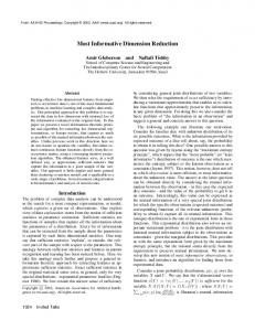
DiReduct Map SNeRV l=0.1

0.9

5NN classification error rate

SNeRV l=0.3 PE

0.8

S−Isomap 0.7

MUHSIC MRE

0.6

NCA 0.5 0.4 0.3 0.2 0.1 0

Letter

Phoneme

Landsat

Fig. 1: Comparison of the 5 nearest neighbor errors for all data sets. assuming Euclidean distance in the projection space. In the following section we evaluate the proposed method using the learning rule based on the t-SNE cost function defined above and locally linear projections obtained by limited rank matrix learning vector quantization (LiRaM LVQ) [4] in a supervised manner.

3

Experiments

In this section we evaluate the proposed method on three data sets also investigated in [12] and described in table 2. For learning locally linear projections, we use LiRaM LVQ with the rank of matrices limited to 10, 10 and 30 for the data sets respectively and the number of prototypes equal to the number of classes. For the coordination, we use crisp responsibilities given by the receptive fields. All other parameters are set as default values. We train the mapping using only a small subset of the full data set (7%-18%) and evaluate the results for the full data set by using the mapping. For evaluation we measure the classification error of the resulting visualization using a 5-nearest neighbor evaluation (5NN error). We compare our results with the results taken from [12] on the same data sets where six state-of-the art supervised nonlinear embeddings are tested (Supervised neighbor retrieval visualizer (SNeRV), Multiple relational embedding (MRE), Colored maximum variance unfolding (MUHSIC), Supervised isomap (S-Isomap), Parametric embedding (PE), Neighbourhood component analysis (NCA)). Note that these methods use only a small subpart of the dataset within an evaluation, while we evaluate our approach on the full data set by means of the explicit mapping. The comparison of the error rates are shown in Figure 1. Interestingly, the classification error obtained by the proposed method is smaller than the alternatives for all three data sets. This is particularly remarkable since we used only a fraction of the data to obtain the map, i.e. the proposed method displays excellent and very efficient generalization to large data sets. The corresponding visualizations display a clear class structure as shown in Figure 2.

4

Conclusion

We have proposed a general way to extend arbitrary dimension reduction techniques, based on cost optimization, to explicit mappings which take into account

285

ESANN 2011 proceedings, European Symposium on Artificial Neural Networks, Computational Intelligence and Machine Learning. Bruges (Belgium), 27-29 April 2011, i6doc.com publ., ISBN 978-2-87419-044-5. Available from http://www.i6doc.com/en/livre/?GCOI=28001100817300.

Letter M M WM M M MM M M M M MM M M M M M M M M M M M M M M M M M M M M M M M M M M W M M M UN M MMMM M M AUM N N

Phoneme prototypes

U J MU UU U R U X A U U U U U U W UU U A U K U U U U C U U U A UU X U U U JAC U U U X U U U U A U U W U UU U U A K Y N OOSO HF N D B M O UD O KG Q O O I N G N B Q N QQ N N O M N N Q O N N R N D O S OG N S Q N Q Q O RYNN QQ Q O O P O O O LQ K G O X N N N K X Q O O Y O N N O Q HN O N L W N J N NNN D Q O O N Q NNN Q Q Q N N Q N Q J N Q O J Q O O O N O D O O OO Q C J O N Q N U N P N N Q Q J Q Q O Q O Q Q O Q Q QQ NN N N O N Q L O P O S Q O O O W O O Q LQ C M Q N W OC H M NN WN JO O H O O O JK Q PQ M C NN LCO R J O JH O SK RR R H O H H H G R KHY H H H H H R G G G H R O K J YH G GH V G R X R G H R R B H I K H A H K K G H T R H G HH G R R R KH G RK R K H KKL H B V W L D G K G HKR G R GG H H HH K G J H H G IR G R R G E K Y H G C R R P R Q R Y HK G R R G G H G G R G D R G T G G K Q G G G R Q H I R R R R H R R G Q G R G I B X M R C G K R H K G G G G R HHH RRRR E TX MH G UH K H KC G K G Q K G KK K KK K K E K K K X K K L P K K K K K BU K K K K K R K X IK K X R H T K K K K R K B E X R K R B B E B GC B D O B D D B B B S G K BB B B G C UM B B E C B B S B B C L S B S B FB E C B C G B E Y B B F B B C K F Y B F C B X C C C C H C B C C C S B N S X T C B B B X B S N E FE BBB E E E C C CCC V H E E C S XX B G E CC EE E C C E C L C C U C C E U G Z X F C T C L EZTB C T E E C XX X K T E E E E E D CW K E C EE C D E F C E HF C D F E C X C E X C B E E G DD C Q X E CCC C E X X O T Q X X X L G X X Q S D CC B E C J E X CC S G O JJ G CCCC X D XG FE D ID H K EE E FXF X X X D X K D H X D D G H D WE X X R D X D X K E X D DD Y X D X D O X R S D D D X X X D X B P D D X P F IK K H D D ID D X X D D LXTTT R D DDD D O HD FE FD M U D H D XXZS X R U D I M R T Y T B T T Z H Y E TTT TT T SS U T TT D T LTFX H T T TT T S T SSS S T X A TT T T B T S S X TTTT S SL G TZ S T EL S S Y J ST SS A I T T L TT T A Y S H S S B A A A S T T X A S U A A A LL S LL L A S AA LLL A S SS A S ISS A S S Z LL A Q A A L LL LLL L S T S A S A A A A A L A A A A L A L SSS A S L A LJ L L A A Q A LL L SH LL A LL A L AAA LLL QA A B Y Q A F F Y Y MY Y YYY YY QLN LLQL Y H AA Y A Y YY Y Y YYY Y Y F Y Y Y F Y Y F Y Y Y Y Y E J Y Y F F Y F Y F Z F LT F FFF YY F FFF Z Y P P Y Y Y ZZZZ VYVV JEE F F F P F F F O F Q F F F Q F Z J L Z YYYP T Z F Z F F S F S F G Z Z Z F QY V BP ZZZS ZZ ER Z FF Z S FFF Q D Z Z T SZS ZZ P IFSYFJFPP Z Z Z FFF P Z R Z Z Z Z S P Z X S I P Z P Z Q Z Y VV Z P P F Z Z Z Z P Q Z Z S P P V P S B F Z Z PP VV FP P B D V ZZZZ IIIIIIIIIIIIIIIIIIIIIII II EZQS P PP P F P V P P P YVVV V ZZ V V P PP P P P P Y KP P Z FPA P G P P P P P P P V V V V P V P V V V VV VV IIIIIIIIIIJII H V V VV V V V V V V V Y V V YPPPPPPP V V V SI VV V V G A JJJX JJJ JJ JJJJJJJJ J JJ J W JJJJJ J WW W JJ J JJJJJ W W W SJ J W W W W W W W W W WM W R W W U W W W W W W W WW W U W W M Q M WW O W W W W W VW W M W W W W W W W F W CMA KW

1 2 3 4 5 6 7 8 9 10 11 12 13

Fig. 2: Visualization of the Letter and Phoneme data set in two dimensions as obtained by the proposed supervised dimension reduction mapping. prior class labeling. We demonstrated the feasibility of the approach for locally linear maps obtained from matrix learning vector quantization and the t-SNE cost function for their coordination, yielding excellent results for three benchmarks. This technique offers the possibility of very flexible and very efficient visualization, since a bias towards given information can easily be integrated into the form of the mapping function and initial solutions, on the one hand, and a small number of data is sufficient to obtain a visualization of the full data set due to the excellent generalization ability of the technique. Acknowledgment This work was supported by the ”Nederlandse organisatie voor Wetenschappelijke Onderzoek (NWO)“ under project code 612.066.620 and by the ”German Science Foundation (DFG)“ under grant number HA-2719/4-1. Further, financial support from the Cluster of Excellence 277 Cognitive Interaction Technology funded in the framework of the German Excellence Initiative is gratefully acknowledged.

References [1] C. Bishop. Pattern Recognition and Machine Learning. Springer, 2007. [2] C. M. Bishop and C. K. I. Williams. GTM: The generative topographic mapping. Neural Computation, 10:215–234, 1998. [3] M. Brand. Charting a manifold. In Advances in Neural Information Processing Systems NIPS 15, pages 961–968. MIT Press, 2003. [4] K. Bunte, B. Hammer, A. Wism¨ uller, and M. Biehl. Adaptive local dissimilarity measures for discriminative dimension reduction of labeled data. Neurocomputing, 73(7-9):1074– 1092, 2010. [5] T. Kohonen. Self-organizing Maps. Springer, 1995. [6] J. Lee and M. Verleysen. Nonlinear dimensionality reduction. Springer, 1st edition, 2007. [7] R. M¨ oller and H. Hoffmann. An extension of neural gas to local PCA. Neurocomputing, 62(305-326), 2004. [8] P. Schneider, M. Biehl, and B. Hammer. Adaptive relevance matrices in learning vector quantization. Neural Computation, 21(12):3532–3561, 2009. [9] Y. W. Teh and S. Roweis. Automatic alignment of local representations. In Advances in Neural Information Processing Systems 15, pages 841–848. MIT Press, 2003. [10] L. J. P. van der Maaten. Learning a parametric embedding by preserving local structure. In 12th AI-STATS, number 5, pages 384–391. JMLR W&CP, 2009. [11] L. J. P. van der Maaten and G. Hinton. Visualizing data using t-SNE. Journal of Machine Learning Research, 9:2579–2605, November 2008. [12] J. Venna, J. Peltonen, K. Nybo, H. Aidos, and S. Kaski. Information retrieval perspective to nonlinear dimensionality reduction for data visualization. Journal of Machine Learning Research, 11:451–490, March 2010.

286