Supplement of Hydrol. Earth Syst. Sci., 20, 3183–3191, 2016 http://www.hydrol-earth-syst-sci.net/20/3183/2016/ doi:10.5194/hess-20-3183-2016-supplement © Author(s) 2016. CC Attribution 3.0 License.
Supplement of Technical note: Multiple wavelet coherence for untangling scale-specific and localized multivariate relationships in geosciences Wei Hu and Bing Cheng Si Correspondence to: Wei Hu (
[email protected]) and Bing Cheng Si (
[email protected])
The copyright of individual parts of the supplement might differ from the CC-BY 3.0 licence.
16 17 18
S1 Calculation of smoothed auto- and cross-wavelet power spectra
19
auto- and cross-wavelet power spectra. Detailed information on the calculations of
20
wavelet coefficients, cross-wavelet power spectra, and bivariate wavelet coherence can
21
be found elsewhere (Kumar and Foufoula-Georgiou, 1997; Torrence and Compo, 1998;
22
Torrence and Webster, 1999; Grinsted et al., 2004; Das and Mohanty, 2008; Si, 2008).
23
The smoothed auto- and cross-wavelet power spectra require the calculation of wavelet
24
coefficients, at different scales and spatial (or temporal) locations, for the response
25
variable and all predictor variables. For convenience, only spatial variables will be
26
referred to, as temporal variables can be similarly analyzed.
In this section, we will only introduce the basics related to the calculation of smoothed
27
The continuous wavelet transform (CWT) of a spatial variable X1 of length N (X1h,
28
h=1, 2, …, N) with equal incremental distance x , can be calculated as the convolution
29
of X1h with the scaled and normalized wavelet (Torrence and Compo, 1998)
W X 1 s ,
30 X1
x N x X 1h h , s 1 s
(1)
s, is the wavelet coefficient of spatial variable X1 at scale s and location
31
where W
32
, and
33
because it allows for the identification of both location-specific amplitude and phase
34
information at different scales in a spatial series (Torrence and Compo, 1998). The
35
Morlet wavelet can be expressed as (Grinsted et al., 2004)
36
1/ 4 ei 0.5 ,
is the mother wavelet function. The Morlet wavelet is used in the CWT
2
37
(2)
where and are the dimensionless frequency and space ( s / x ), respectively.
38
The auto-wavelet power spectrum of spatial variable X1 can be expressed as
39
W X1 , X1 s , W X1 s , W X1 s , ,
40
X where W 1 s, is a complex conjugate of W
41
expressed as the squared amplitude of W
46 47 48
s, , which is 2
(4)
The cross-wavelet spectrum between spatial variables of Y and X1 can be defined as
W Y , X1 s , W Y s , W X1 s , ,
44 45
s, . Therefore, Eq. (3) can also be
W X 1 , X 1 s , W X 1 s , .
42 43
X1
X1
(3)
where W
Y
(5)
s, is the wavelet coefficient of spatial variable Y.
Both the auto- and cross-wavelet spectra can be smoothed using the method suggested by Torrence and Compo (1998), W s, SM scale SM space W s, ,
(6)
49
where is a smoothing operator. SM scale and SM space indicate the smoothing along the
50
wavelet scale axis and spatial distance, respectively (Si, 2008). The W is the normalized
51
real Morlet wavelet and has a similar footprint as the Morlet wavelet
52 53 54
1 2 / 2 s2 e . s 2
(7)
Therefore, the smoothing along spatial distance can be calculated as N xk 2 / 2 s2 1 SM scale W s, W s, e s, s 2 k 1
(8)
2s 2 2
represents a fixed s value. The Fourier transform of Eq. (7) is e
55
where
56
Therefore, Eq. (8) can be implemented using Fast Fourier Transform (FFT) and Inverse
57
Fast Fourier Transform (IFFT) based on the convolution theorem, and is written as
58 59
s
2 s2 2 SM scale W s, x IFFT FFT W s, x e .
.
(9)
The smoothing along scales is then written as [Torrence and Compo, 1998]
1 k m SMspace W sl , x 0.6sl 2m 1 l k m
60
SM scale W sk , x
61
where is the rectangle function,
62
scales. The coefficient of 0.6 is the empirically determined scale decorrelation length for
63
the Morlet wavelet (Torrence and Compo, 1998).
x
x
,
(10)
indicates a fixed x value, and l is the index for the
64 65 66 67 68 69 70 71 72 73 74 75 76 77 78 79 80 81 82 83 84 85 86 87 88 89 90 91 92 93 94 95 96 97 98 99 100 101 102 103 104
S2 Matlab code for MWC (mwc.m) % This is a Matlab code (mwc.m) for calculating multiple wavelet coherence. % Please copy the following content into a txt file and rename it to “mwc.m” prior to running.
function varargout=mwc(X,varargin) % Multiple Wavelet coherence % Creates a figure of multiple wavelet coherence % USAGE: [Rsq,period,scale,coi,sig95]=mwc(X,[,settings]) % % Input: X: a matrix of multiple variables equally distributed in space %
or time. The first column corresponds to the dependent variable,
%
and the second and consequent columns are independent variables.
% % Settings: Pad: pad the time series with zeros? %.
Dj: Octaves per scale (default: '1/12')
%.
S0: Minimum scale
%.
J1: Total number of scales
%.
Mother: Mother wavelet (default 'morlet')
%.
MaxScale: An easier way of specifying J1
%.
MakeFigure: Make a figure or simply return the output.
%.
BlackandWhite: Create black and white figures
%.
AR1: the ar1 coefficients of the series
%. %.
(default='auto' using a naive ar1 estimator. See ar1nv.m) MonteCarloCount: Number of surrogate data sets in the significance calculation. (default=1000)
% Settings can also be specified using abbreviations. e.g. ms=MaxScale. % For detailed help on some parameters type help wavelet. % Example: %
t=[1:200]';
%
mwc([sin(t),sin(t.*cos(t*.01)),cos(t.*sin(t*.01))])
% Please acknowledge the use of this software package in any publications, % by including text such as:
% "The software for the multiple wavelet coherence was provided by W. Hu % and B. Si, and is available in the Supplement of Hu and Si (2016)." % and cite the paper: % "Hu, W., and B. Si (2016), Technical Note: Multiple wavelet coherence for untangling scale-specific and localized % multivariate relationships in geosciences, Hydrol. Earth Syst. Sci., volume and page numbers to be allocated."
105 106 107 108 109 110 111 112 113 114 115 116 117 118 119 120 121 122 123 124 125 126 127 128 129 130 131 132 133 134 135 136 137 138 139 140 141 142 143 144 145 146
% (C) W. Hu and B. Si 2016 % % ----------------------------------------------------------% % Copyright (C) 2016, W. Hu and B. Si 2016 % This software may be used, copied, or redistributed as long as it is not % sold and this copyright notice is reproduced on each copy made. This % routine is provided as is without any express or implied warranties % whatsoever. % %
Wavelet software was provided by C. Torrence and G. Compo,
%
and is available at URL: http://paos.colorado.edu/research/wavelets/.
% %
Crosswavelet and wavelet coherence software were provided by
%
A. Grinsted and is available at URL:
%
http://www.glaciology.net/wavelet-coherence
% % We acknowledge Aslak Grinsted for his wavelet coherency code (wtc.m) on % which this code builds. % %----------------parse function arguments-----------------------------------------------------
[row,col]=size(X); [y,dt]=formatts(X(:,1)); mm=y(1,1); nn=y(end,1);
for i=2:col; [x,dtx]=formatts(X(:,i));
if (dt~=dtx) error('timestep must be equal between time series'); end
mm1=x(1,1); nn1=x(end,1);
if mm1>mm mm=mm1; end
if nn1=(t(1)-dte))&(y(:,1)=(t(1))-dte)&(x1(:,(i-1))0)||(Args.MakeFigure)
271 272 273 274 275 276 277 278 279 280 281 282 283 284 285 286 287 288 289 290 291 292 293 294 295 296 297 298 299 300 301 302 303 304 305 306 307 308 309 310 311 312
mwcsig=mwcsignif(Args.MonteCarloCount,Args.AR1,dt,length(t)*2,Args.Pad,Args.Dj,Args.S0,Args.J1,Args.Mother,. 6); mwcsig=(mwcsig(:,2))*(ones(1,n)); mwcsig=Rsq./mwcsig; end
if Args.MakeFigure
Yticks = 2.^(fix(log2(min(period))):fix(log2(max(period))));
if Args.BlackandWhite levels = [0 0.5 0.7 0.8 0.9 1]; [cout,H]=safecontourf(t,log2(period),Rsq,levels);
colorbarf(cout,H) cmap=[0 1;.5 .9;.8 .8;.9 .6;1 .5]; cmap=interp1(cmap(:,1),cmap(:,2),(0:.1:1)'); cmap=cmap(:,[1 1 1]); colormap(cmap) set(gca,'YLim',log2([min(period),max(period)]), ... 'YDir','reverse', 'layer','top', ... 'YTick',log2(Yticks(:)), ... 'YTickLabel',num2str(Yticks'), ... 'layer','top'); ylabel('Period'); hold on
if ~all(isnan(mwcsig)) [c,h] = contour(t,log2(period),mwcsig,[1 1],'k');%#ok set(h,'linewidth',2); end %suptitle([sTitle ' coherence']); %plot(t,log2(coi),'k','linewidth',2) tt=[t([1 1])-dt*.5;t;t([end end])+dt*.5]; %hcoi=fill(tt,log2([period([end 1]) coi period([1 end])])); %hatching- modified by Ng and Kwok hcoi=fill(tt,log2([period([end 1]) coi period([1 end])]),'w');
hatch(hcoi,45,[0 0 0]); hatch(hcoi,135,[0 0 0]); set(hcoi,'alphadatamapping','direct','facealpha',.5);
313 314 315 316 317 318 319 320 321 322 323 324 325 326 327 328 329 330 331 332 333 334 335 336 337 338 339 340 341 342 343 344 345 346 347 348 349 350 351 352 353 354
plot(t,log2(coi),'color','black','linewidth',1.5); hold off else H=imagesc(t,log2(period),Rsq);%#ok %[c,H]=safecontourf(t,log2(period),Rsq,[0:.05:1]); %set(H,'linestyle','none')
set(gca,'clim',[0 1]);
HCB=safecolorbar;%#ok
set(gca,'YLim',log2([min(period),max(period)]), ... 'YDir','reverse', 'layer','top', ... 'YTick',log2(Yticks(:)), ... 'YTickLabel',num2str(Yticks'), ... 'layer','top'); ylabel('Period'); hold on
if ~all(isnan(mwcsig)) [c,h] = contour(t,log2(period),mwcsig,[1 1],'k');%#ok set(h,'linewidth',2); end %suptitle([sTitle ' coherence']); tt=[t([1 1])-dt*.5;t;t([end end])+dt*.5]; hcoi=fill(tt,log2([period([end 1]) coi period([1 end])]),'w'); set(hcoi,'alphadatamapping','direct','facealpha',.5); hold off end end %---------------------------------------------------------------%
varargout={Rsq,period,scale,coi,mwcsig}; varargout=varargout(1:nargout);
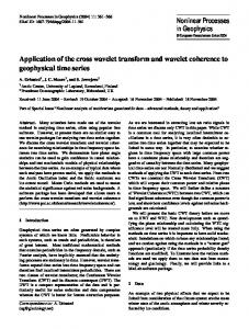
function [cout,H]=safecontourf(varargin) vv=sscanf(version,'%i.'); if (version('-release')32 months) scales,
666
while temperature was the dominating factor at the medium (8–32 months) scales (Fig.
667
S2). The relative humidity corresponded to the greatest mean MWC (0.62) and PASC
668
value (40%) at multiple scale-location domains.
669
The evaporation from free water surface was significantly correlated to each
670 671 672 673 674 675 676 677 678 679 680 681
Figure S2. Bivariate wavelet coherency between evaporation (E) from water surfaces and each of the meteorological factors (relative humidity, mean temperature, sun hours, and wind speed) at Changwu site in Shaanxi, China. Arrows show the correlation type with the right pointing arrows being positive and left pointing arrows being negative. Thin solid lines demarcate the cones of influence and thick solid lines show the 95% confidence levels.
682
References
683 684
Das, N.N. and Mohanty, B. P.: Temporal dynamics of PSR-based soil moisture across
685
spatial scales in an agricultural landscape during SMEX02: A wavelet approach, Remote
686
Sens. Environ., 112, 522–534, doi:10.1016/j.rse.2007.05.007, 2008.
687
Grinsted, A., Moore, J. C., and Jevrejeva, S.: Application of the cross wavelet transform
688
and wavelet coherence to geophysical time series, Nonlinear Proc. Geoph., 11, 561–566,
689
2004.
690
Hu, W. and Si, B. C.: Soil water prediction based on its scale-specific control using
691
multivariate empirical mode decomposition, Geoderma, 193–194,180–188, doi:
692
10.1016/j.geoderma.2012.10.021, 2013.
693
Kumar, P. and Foufoula-Georgiou, E.: Wavelet analysis for geophysical applications,
694
Rev. Geophys., 35, 385–412, doi: 10.1029/97RG00427, 1997.
695
She, D. L., Tang, S. Q., Shao, M. A., Yu, S. E., and Xia, Y. Q.: Characterizing scale
696
specific depth persistence of soil water content along two landscape transects, J. Hydrol.,
697
519, 1149–1161, doi:10.1016/j.jhydrol.2014.08.034, 2014.
698
Si, B. C.: Spatial scaling analyses of soil physical properties: A review of spectral and
699
wavelet methods, Vadose Zone J., 7, 547–562, doi: 10.2136/vzj2007.0040, 2008.
700
Torrence, C. and Compo, G. P.: A practical guide to wavelet analysis, Bull. Am.
701
Meteorol. Soc., 79, 61–78, doi: 10.1175/1520-0477(1998)0792.0.co;2,
702
1998.
703
Torrence, C. and Webster, P. J.: Interdecadal changes in the ENSO-monsoon system, J.
704
Clim., 12, 2679–2690, doi: 10.1175/1520-0442(1999)0122.0.CO;2,
705
1999.