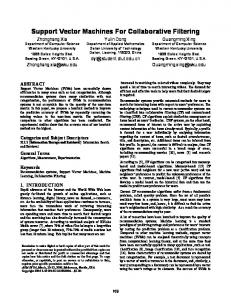
The surface approximation is based on a modified Support Vector regression. We present ... point cloud of surface points as training data (Figure 1). This.
EUROGRAPHICS 2005 / M. Alexa and J. Marks (Guest Editors)
Volume 24 (2005), Number 3
Support Vector Machines for 3D Shape Processing Florian Steinke,1 Bernhard Schölkopf1 and Volker Blanz2 1
Max-Planck-Institut für biologische Kybernetik, Tübingen, Germany 2 Max-Planck-Institut für Informatik, Saarbrücken, Germany
Abstract We propose statistical learning methods for approximating implicit surfaces and computing dense 3D deformation fields. Our approach is based on Support Vector (SV) Machines, which are state of the art in machine learning. It is straightforward to implement and computationally competitive; its parameters can be automatically set using standard machine learning methods. The surface approximation is based on a modified Support Vector regression. We present applications to 3D head reconstruction, including automatic removal of outliers and hole filling. In a second step, we build on our SV representation to compute dense 3D deformation fields between two objects. The fields are computed using a generalized SV Machine enforcing correspondence between the previously learned implicit SV object representations, as well as correspondences between feature points if such points are available. We apply the method to the morphing of 3D heads and other objects. Categories and Subject Descriptors (according to ACM CCS): I.3.5 [Computer Graphics]: Computational Geometry and Object Modeling — Curve, surface, solid, and object representation
1. Introduction During recent years, statistical learning techniques have attracted increasing attention in various disciplines of computer science. Learning methods are in general applicable in all situations where empirical training data are available, and a generalization to novel instances has to be established. Depending on the complexity of the functional dependency to be estimated, this can be achieved by low-dimensional parametric models, or by more general, non-parametric methods. A particular class of non-parametric methods which have become popular in machine learning and statistics are kernel methods or kernel machines [SS02]. All kernel methods, including the well-known Support Vector Machine (SVM) [Vap98], share the use of a positive definite kernel k : X × X → R. Here, X is the domain in which the empirical data live. In pattern recognition, say, X might be a vector space of images. In this paper, we assume X to be R3 or a subset thereof, containing the point cloud samples and the implicit surface. Positive definite kernels are characterized by the property that there exists a mapping Φ from X into a Hilbert space H (termed the reproducing kernel Hilbert c The Eurographics Association and Blackwell Publishing 2005. Published by Blackwell
Publishing, 9600 Garsington Road, Oxford OX4 2DQ, UK and 350 Main Street, Malden, MA 02148, USA.
y
h3
Φ(x) xx
z
Implicit Surface in R
3
x
h2 h1
Hyperplane in Hilbert Space
Figure 1: The mapping Φ defined by the kernel function k (Equation 1) transforms the 3D surface to a hyperplane in a high-dimensional Hilbert space. space associated with k) such that for all x, x0 ∈ X ,
� k(x, x0 ) = Φ(x), Φ(x0 ) .
(1)
Eq. (1) has far-reaching consequences. It implies that whenever we have an algorithm that can be carried out in terms of inner products — essentially, all algorithms that can be formulated in terms of distances, lengths, and angles — we can construct a nonlinear generalization of that algorithm by substituting a suitable kernel for the usual inner product.
F. Steinke, B. Schölkopf & V. Blanz / Support Vector Machines for 3D Shape Processing
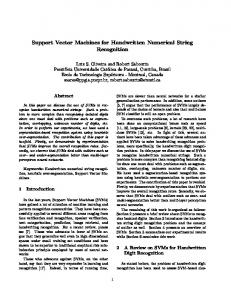
rithms approximate the signed distance function by the discretized solution of partial differential equations and apply it to surface editing applications [MBWB02]. Another powerful class are methods based on local approximations of the surface, such as Moving-Least-Squares methods [ABCO∗ 03, PKKG03, SOS04] and Multi-level Partition of Unity [OBA∗ 03]. Figure 2: The second algorithm presented in this paper computes a dense correspondence (dashed arrows) between two regions containing the surfaces (shaded gray) by matching implicit surface representations and given additional pairs of corresponding feature points (black circles). Implicitly, we are then carrying out the algorithm in the (possibly infinite-dimensional) Hilbert space H. The core idea of kernel methods is thus to reduce complex nonlinear learning problems to linear estimation problems in Hilbert spaces. For instance, in SVM classifiers, the elements of two classes are separated by a hyperplane in H. SVM classifiers form a very general class of learning machines, and they include many common types of neural networks as a special case, e.g., 2-layer feedforward networks and radial basis function (RBF) networks. In this paper, we present a method that represents the surface of a 3D object in terms of a hyperplane in H, given a point cloud of surface points as training data (Figure 1). This implicit surface can be used for smoothing, de-noising and hole filling. We then take the approach one step further by learning a kernel based deformation mapping which, given two objects implicitly represented by kernel machines, will transform one into the other (i.e., a warp field). If pairs of feature point correspondences are available for guiding the warp field, they are taken into account by the algorithm. Unlike most previous methods for surface correspondence, our method provides an estimate of correspondence in the 3D volume around the surface (Figure 2). For human faces, this can be used for warping additional structures, such as the eyeglasses shown in the supplemental material, or anatomical structures inside of the head, such as teeth or bone structures. Our new technique can be applied not only for visual effects, but also in medicine or for scientific visualization and modeling of volume data. The next section briefly reviews related work. Section 3 presents our approach for SVM surface reconstruction. Section 4 describes the kernel based deformation mapping between implicit surfaces. Section 5 gives experimental results on both proposed approaches, and we conclude with a discussion of our findings (Section 6). 2. Related work The approaches to the construction of implicit surface representations can be divided into three groups: Some algo-
The third class, into which our own method falls, use a global representation of the implicit surface function based on an expansion in radial basis functions (RBF). Some authors have proposed non-compactly supported basis functions [CBC∗ 01, TO99], others have used compactly supported basis functions [MTR∗ 01, OBS03] as we do. Unlike these methods, which perform a least-squares approximation with a regularization term that avoids over-fitting and produces a smooth result, our implicit function algorithm uses a distance function that is more robust towards outliers, and another approach for controlling smoothness that is derived from machine learning. [WL03] proposed a level set estimation method using an SVM classifier for 2D outline estimation in computer vision. [SGS05] recently presented an algorithm which is based on one-class classifiers. Both methods do not attempt to approximate the signed distance, nor do they scale well enough to be applied to datasets such as the largest in the present paper. Automated algorithms for computing point-to-point correspondences between surfaces have been presented previously in the context of 3D morphable models. For parameterized surfaces of human faces that were captured with a laser scanner, a modified optical flow algorithm has been proposed [BV99]. On more general shapes such as animals or human bodies, methods have been developed that match each mesh vertex of the first shape to the most similar point on the second mesh [She00, ACP03]. These methods minimize the distance to the target mesh and maximize the smoothness of the deformation in terms of stiffness of the source mesh [She00] or the similarity between transformations of adjacent vertices [ACP03]. For matching partially overlapping portions of the same surface, Iterative Closest Point Algorithms [BM92, RL01] provide a reliable solution. A variety of methods are available from medical data registration [AFP00]. However, these methods do not use implicit functions and machine learning methods. Unlike deformations that are defined only on the surface, a volume deformation algorithm based on free-formdeformations with B-Splines between landmark points has been described for MRI scans of human brains [RF03]. [MKN∗ 04] extend a physically plausible deformation from a set of sample points to the whole object using a Moving Least Squares approach. [COSL98] morph two objects into each other by first applying an elastic deformation based on feature point correspondences and then blending two implicit functions describing the objects into each other. c The Eurographics Association and Blackwell Publishing 2005.
F. Steinke, B. Schölkopf & V. Blanz / Support Vector Machines for 3D Shape Processing
following convex quadratic optimization problem:
3. Surface reconstruction Implicit surface modeling is based on the idea that a surface can be described as the set of all x ∈ X ⊆ RD (D being the dimension of input space) for which a function f : X → R equals zero. The method presented here will model this function as a hyperplane in the (reproducing kernel) Hilbert space H, i.e., as the zero set of the functional f (x) = hw, Φ(x)i + b,
(2)
where w ∈ H, b ∈ R. This hyperplane will approximately pass through the given surface points, mapped into H via Φ. In Section 3.1 we will show how this hyperplane can actually be computed. It will turn out that f can be written as m
f (x) =
∑ αi k(xi , x) + b,
(3)
i=1
where k satisfies (1). We will use a radial basis kernel and call the xi kernel centers or base points. It is clear that one can trivially “solve” this problem by setting w and b to zero. To avoid this, we will include off-surface training points and enforce f to take nonzero values on those points, to be explained in Section 3.2. In Section 3.3 we will describe a multi-scale scheme, and in Section 3.4 we show how the necessary parameters can be selected automatically.
3.1. A Simplified SVM Regression Algorithm Our goal is to fit the function f to a given training set of points x1 , . . . , xm ∈ X and corresponding target values y1 , . . . , ym ∈ R. For surface points, the target values are yi = 0. We use an adaptation of the so-called ε-insensitive SVM regression algorithm [Vap98, SS02]. As a best fit, we find a trade-off between penalization of errors and regularization of the solution via the Hilbert space norm of w. The term kwk2 is often referred to as a large margin regularizer, as its minimization in an SV classifier induces a large margin of separation between the classes. Alternatively, it can be interpreted as enforcing smoothness of the solution (for details, see [SS02]). A difference of the function f (x) = hw, Φ(x)i + b at point xi to the target value yi is penalized linearly as soon as it (∗) exceeds the threshold ε ≥ 0 by a value ξi ≥ 0. This εinsensitive loss function [Vap98] makes the SVM more robust to heavy-tailed noise (such as outliers) than the squared loss regression which is used in standard least-squares approaches [SS02]. With a parameter C > 0 that controls the trade-off between error penalization and function regularization, we obtain the c The Eurographics Association and Blackwell Publishing 2005.
minimize
w∈H,ξi ,ξ∗ i ∈R
1 kwk2 +C ∑ (ξi + ξ∗i ) 2 i
subject to
(4)
hw, Φ(xi )i + b − yi ≤ ε + ξi −hw, Φ(xi )i − b + yi ≤ ε + ξ∗i ξi , ξ∗i ≥ 0
Here and below, indices are assumed to run or to sum over 1, . . . , m by default. In contrast to standard SV regression, we set the offset b to a fixed value (see Section 3.3). This will simplify the dual formulation of the optimization problem. The dual problem is obtained by using the formalism of constrained optimization, known as Lagrange duality for the case of equality constraints and extended by Karush, Kuhn and Tucker (KKT) to the case of inequality constraints (see e.g. [SS02]). A standard calculation leads to: 1 T minimize α Kα + ∑ (αi − α∗i )yi + ε ∑ (αi + α∗i ) (5) αi ,α∗ i ∈R 2 i i subject to
0 ≤ αi , α∗i ≤ C
where α = (α1 − α∗1 , . . . , αm − α∗m )T , Ki j = k(xi , x j ). Using the KKT optimality conditions, it can be shown that the solution satisfies w = ∑m i=1 αi Φ(xi ). Note that unlike (4), this problem does no longer explicitly depend on Φ or any element of H. Together with the kernel equation (1) the hyperplane f can be expressed in terms of kernels (3). This step, which is crucial to all SV methods, reduces the inner product between two possibly infinite-dimensional vectors to an expansion which can be evaluated efficiently. Problem (5) is a convex quadratic program with a positive definite matrix K and a box constraint. We employ a simple coordinate descent optimization scheme, selecting one dimension at a time and optimizing the objective function as a function of that variable with the others fixed: −yi − ε − ∑ j6=i Ki j α j αnew = i Kii If αnew falls out of the interval [0,C] we set it to the closest i feasible point. This update which is similar to the symmetric Gauss-Seidel method can be done very efficiently in constant time, if K is sparse. To ensure sparsity of K, we use the so called Wu function [Sch95] as a kernel, k(r) = (1 − r)4+ (4 + 16r + 12r2 + 3r3 ), kx−yk
where r = σ . It has compact support of size σ > 0 and is in C2 (R3 ). As the result is differentiable, we can calculate higher order differential characteristics of the implicit surface, such as Gaussian or mean curvature [TG95]. While we have presently introduced the optimization problem (5) in a somewhat heuristic fashion, it should be stressed that there are several ways to justify it theoretically: • Uniform convergence bounds are generalizations of the
F. Steinke, B. Schölkopf & V. Blanz / Support Vector Machines for 3D Shape Processing
•
•
•
•
classical law of large numbers which imply that empirical estimates of error rates will converge to true error rates provided certain notions of capacity of function classes are well-behaved. In the case of SV regression, one can show that the quantity kwk2 is such a way to control the capacity of the class of linear functions (2), and one can derive probabilistic upper bounds on the error of the estimated function on previously unseen points (the so-called generalization error). These bounds depend essentially on the training error and the size of kwk2 [Vap98]. Algorithmic Stability is a notion that measures how much the solution of an estimation problem changes if the training set is perturbed. High stability combined with low training error leads to a low generalization error, and, as above, high stability can be related to a small kwk2 [BE01, SS02]. Regularization Theory — a small value of kwk2 can be shown to induce smoothness of the estimated function in a kernel-dependent manner; for details see [SS02]. Compression — for SVM classifiers, one can show that a solution with a small kwk2 can be interpreted as a compression of the training target values, given the input points. This also leads to generalization error bounds [vLBS04]. Bayesian “Maximum A Posteriori” Methods lead to optimization problems of the form (4) and are optimal in the sense of producing the most likely model, given the empirical data, an observation error model, and a prior distribution formulated in terms of kwk2 . We point out that the observation error model underlying the squared loss is a Gaussian, while the ε-insensitive loss used in our method arises from a distribution with heavier tails [SS02], which is better able to model outliers.
3.2. Training Point Generation The goal of this section is to estimate the function f such that it reproduces the signed distance in the vicinity of the surface. This not only helps to avoid trivial solutions f (x) ≡ 0, but also defines a functional surface description that can be used for a variety of purposes, such as collision detection or 3D morphing (Section 4). Similarly to [CBC∗ 01] we achieve this goal by including additional input pairs (xi , yi ) with base points xi on either side of the surface. These additional training points are generated by displacing given surface points along their surface normals by a distance yi , using negative values inside and positive ones outside. The distances along the normals are chosen such that the kernel function k(x) = k(xi , x) has a stable, non vanishing gradient on the supposed surface. When deciding whether to include a thus constructed offsurface point in the training set, we use a heuristic to ensure that its target value yi is approximately within 10% of the correct signed distance. Clearly, the true distance of the point is at most |yi |. However, it may happen that the surface
bends around, and it in fact is closer than this. We discard the point if there exists a surface training point at a distance of less than 0.9|yi |. The method worked well in all our experiments. We assume that surface normals are given, or can be computed from mesh connectivity or nearest neighbor information. The above consistency check and the choice of loss function make the method robust with respect to noise in the normal estimates. It is a well-known and fundamental property of SVMs that in the resulting expansion of f (Equation 3) a large portion of coefficients αi may vanish, so f depends only on a subset of kernel centers xi [SS02] (called SVs). The SVM adapts the density of contributing kernel centers xi to the complexity of the surface. However, it is in general not known before training which points will end up becoming SVs. As a consequence, the runtime of a “vanilla” implementation of SVMs scales like O(m3 ). In our specific problem, however, we can make the optimization algorithm more efficient by pre-selecting points before training: In a box subdivision scheme, an initial bounding box is recursively subdivided to a given resolution defined by the kernel support, and the center points are extracted. That way the number of base points within the support of a kernel function is limited to a fixed number. When solving the optimization problems, it turns out that most of the thus constructed training points will wind up being SVs. The above procedure can thus also be viewed as a way of preprocessing the training set to identify points which are likely to become SVs. For computing the kernel matrix, we apply a fast O(log m) nearest-neighbor searcher, reducing the runtime scaling of this step from O(m2 ) to O(m log m). The same method also guarantees fast evaluation in O(log m) time. The overall training time of our algorithm, including the SVM optimization, is also O(m log m), and the storage requirement is linear, making it applicable to large datasets.
3.3. Multi Scale Approach In order to obtain a simple and smooth solution which can interpolate across holes in the surface, we use a combination of kernels at different sizes. We apply an iterative greedy multi-scale approximation, starting on a very coarse level to approximate the signed distance function. On subsequent finer scales, we only approximate the residual errors. The final function is given as the sum of the functions computed at each level. We set the fixed offset b equal to the biggest kernel width. While iterating through the different scales, we discard a proposed base point if the value of the function at higher levels is already within the desired fitting accuracy. As larger kernels can describe flat regions rather well, the number of base points automatically adapts to the complexity of the object. c The Eurographics Association and Blackwell Publishing 2005.
F. Steinke, B. Schölkopf & V. Blanz / Support Vector Machines for 3D Shape Processing
Figure 4: Holes due to occlusions in the scanning process (left) are filled by the implicit surface (right).
Figure 3: An implicit surface reconstruction of the dragon of the Stanford 3D Scanning Repository. The original mesh has more than 400k data points. Our reconstruction uses 280k kernel centers.
3.4. Parameter Selection The system parameters can be determined without user interaction. For the kernel widths at different scales, we use a cascade of 1/2, 1/4, ... of the diameter of the object. This choice provides the model with enough variability to reconstruct fine details while reliably extrapolating across larger distances. Refinement stops automatically when no new base points are added any more, i.e. when all proposed base points are within the desired fitting accuracy. For our test datasets, five to six scales gave visually plausible and precise results. The regularization parameters are more difficult to determine. We use a simple validation scheme: In this scheme, only a subset of points are used for fitting, while the others are independent data to test the generalization error. If the relative weight of the regularizer is too high (small C in (4)), the function is smooth but does not fit the training data. If, on the other hand, the loss term of the objective function is given too much weight (large C in (4)), we experience overfitting and the generalization to non-training points deteriorates. We find the optimal weight by measuring the generalization error for different values. The optimal parameter values transfer well across a broad class of objects. 4. Dense 3D Deformation Fields Finding a deformation field for morphing objects and, more generally, defining a criterion for correct correspondence between surfaces are challenging problems. The algorithm presented in this section computes a smooth 3D deformation field between two implicit surfaces. Unlike most other methods, it gives an estimate of deformation not only on the surface, but on the entire 3D volume that embeds it, which can be useful for a large range of applications not only in graphics, but also in medicine and engineering. c The Eurographics Association and Blackwell Publishing 2005.
The mapping computed by the proposed algorithm preserves the value of the function implicitly describing the object not only on the surface f (x) = 0, but also on offsurface points. By construction, this implies that it preserves the value of the signed distance function. Whilst we found this to work rather well, performance can in some cases be improved by enforcing invariance of additional quantities, such as derivatives of the signed distance function. For further details, see [SSB05]. In many applications, point-wise correspondences are easy to find, such as the tip of the nose in faces. The challenge then is to extend these into a complete correspondence field for all on- and off-surface points. In our approach, we assume our objects to be aligned and scaled to the same size (there is a number of algorithms to solve the registration problem given a few correspondences [HS92]). Suppose (xi , zi ) ∈ X × X , i = 1, . . . , m, are corresponding point pairs, where the xi lie on the first and the zi on the second object. We use the transformation x 7→ x + τ(x)
(6)
with the displacement field τ : X → X minimizing m 1 D kwd k2 +Ccorr ∑ kxi + τ(xi ) − zi k2 ∑ 2 d=1 i=1
+Cdist
Z
X
| f1 (x) − f2 (x + τ(x))|2 dx
(7)
over the wd ∈ H, where (following the SVM approach) we model each coordinate of τ as a linear functional τd (x) = hwd , φ(x)i, corresponding to a hyperplane in H. The first term of (7) is the large margin (or smoothness) term of SVMs, and the second term penalizes errors in the known corresponding point pairs. The third term uses the functions f1 , f2 implicitly describing the two objects, respectively. Since these functions are constructed using the method of Section 3, they approximate the signed distance function. Therefore, minimizing this term will lead to a deformation τ which preserves signed distances: points will tend to get mapped to points with the same distance to the (new) surface.
F. Steinke, B. Schölkopf & V. Blanz / Support Vector Machines for 3D Shape Processing
Figure 5: A head model reconstruction with different regularization parameters. The left image uses the parameters chosen by the automatic validation procedure proposed in Section 3.4, which leads to accurate results. For some applications, a smoother surface (center) may be preferable. Additional smoothing without re-fitting can be obtained by just excluding the finest scales during evaluation as demonstrated in the right figure.
Figure 6: The outlier noise in the left scan was automatically removed with our method using a linear loss function (center). For the squared loss function (right) even the best parameter set produced some spurious surfaces. In (7), the integral is taken over the whole domain X on which we want to use the warp. To turn this into a practical problem, we first convert the integral into a finite sum by sampling points, say from the area on and around the surface. Moreover, if we set Cdist to zero initially, the problem can be decomposed into D convex quadratic programs for wd corresponding to SVMs with squared loss function. Taking this as an initial solution, we then optimize the dual of (7) using gradient descent. We use the same kernel as above and also apply a multiscale scheme. In order to make sure that the sparse feature point correspondences lead to a good initial guess in a larger vicinity, we apply wide kernels. For matching detail structures on the surface of the second object, we need enough flexibility in the model as provided by smaller kernels. We iterate the optimization procedure from coarse to fine and take each level’s results as the initial solution for the next level.
Although the problem of warp field estimation looks rather different from the implicit surface estimation problem, the optimization problems and the multi-scale strategies are rather similar, enabling us to re-use almost all of our code.
5. Experimental Results We have tested our method on a number of 3D objects, such as the dragon model of the Stanford 3D Scanning Repository (see Figure 3), and on scans of human faces from laser or structured light scanners. To visualize our implicit surfaces, we use a surfacefollowing version of the standard Marching Cubes algorithm. Speed. We tested our algorithm for surface reconstruction on different sub-samplings of the head model in (Figure 5) as well as the dragon (Figure 3). The fitting accuracy was c The Eurographics Association and Blackwell Publishing 2005.
F. Steinke, B. Schölkopf & V. Blanz / Support Vector Machines for 3D Shape Processing
Figure 7: A warp between the left triangle and the middle/right figure (black lines). The function values of the implicit surface functions are color coded. We mark 3 correspondences (red squares) on both objects and visualize the warp on a number of test points (black crosses). In the center image, the warp is estimated just from the given correspondences, i.e., without our distance to surface error term. Points between the triangles’ corners do not fall on the target shape. With the distance to surface term (right), the warp maps surface points to surface points. The distance to the surface is preserved for off-surface points. set to 0.1% of the object diameter. The times presented here include the entire process of base point generation and optimization on 6 scales. All tests were run on an Intel Pentium 4 2.2 GHz processor with 1 GB RAM. Object Head Head Head Head dragon
# Points 2509 15k 51k 178k 405k
Time [s] 3.4 12.4 23.3 34.9 319
# Kernel centers 7797 20297 25563 30162 284003
For a given data set, the number of kernel centers saturates (cf. numbers of the head model) as the number of input surface points increases. Flat, densely sampled regions can already be approximated with a few large kernels, so a larger number of points does not increase precision. The algorithm discards them during the base point generation procedure on finer scales. If, on the other hand, the structures of the object are more complex (e.g., the dragon model), then the number of required kernel centers increases significantly, which demonstrates how our algorithm automatically adapts to the object’s complexity. We tried to compare the implementation of our method with the state of the art FastRBF code of [CBC∗ 01]. Trial versions of this system are available in public domain. The authors of [CBC∗ 01] have told us that there is a multi-scale version of their system, but the code available to us does not include that. It produces large numbers of RBF centers which makes a fair comparison difficult. For the head model with 50k input points the run time was more than 7 min using more than 100k RBF centers. In cases where both methods used the same number of kernel centers for optimization, our code ran about two to three times faster than the FastRBF code. This is probably due to the fact that our optimization procedure is extremely simple (in fact, the core procedure is only 15 lines of C++ code) whereas [CBC∗ 01] use sophistic The Eurographics Association and Blackwell Publishing 2005.
cated approximation schemes to handle non-compactly supported RBF functions. Smoothing, Denoising, Hole filling A common application of implicit surface representations is interpolation across holes and smoothing of real world datasets. As demonstrated in Figures 4 and 5, our method solves both tasks equally well. Unlike most other methods, which rely on a squared loss function, our results are relatively robust with respect to outlier noise, which is a common phenomenon in raw data of many types of scanners. Our SVM approach is based on a robust error measure which weighs large deviations less strongly than squared error measures would. The effect of different loss functions is demonstrated in Figure 6. When using a squared loss function in our algorithm, a 3D dataset with huge outliers (an original scan from a structured-light scanner) did not yield acceptable results, while our SVM method could deal with this dataset with only a minor change of the parameter set. Signed distance function For the construction of 3D warp fields, we rely on the fact that our implicit representation locally approximates the signed distance function. We evaluated the quality of this approximation by plotting the function value for points shifted along the surface normals (Figure 8). The diagram indicates that the function values are a good approximation to the signed distance up to about 15% of the object’s diameter. The validity range can be increased by including larger kernels into the multi-scale iteration. Deformation fields Figure 7 demonstrates our deformation field algorithm in a simple toy environment. We fit implicit surface functions to two shapes, and construct a warp field using three given correspondence pairs. We show its effect on some test points. If we neglect our distance to surface error term in (7) the best warp is one which maps the corresponding points onto each other and leaves the geometry of the object unchanged as far as pos-
F. Steinke, B. Schölkopf & V. Blanz / Support Vector Machines for 3D Shape Processing
A B C D E F Start 50% 100% Target No Correspondence Features only Figure 9: A morph between two faces (A and D, with markers). Figures B and C show intermediate morphs of the mesh vertices. Note that the 100% image equals the target image D precisely. Figure E shows a 50% morph without correspondences where the surface is just projected from face A to D, producing ghost structures (e.g., a double mouth). Figure F shows an elastic deformation just using the point correspondences without the distance-to-surface error term: The corresponding points are mapped accurately, but the overall face structure is not aligned with the target D.
Start Target 25% 50% 75% 100% Figure 10: The Stanford bunny’s head morphed into a human head. We used the same technique as in Figure 9.
The second example shows a morph between two 3D heads. We defined 18 correspondences on distinct feature points as well as on the borders of the shape. Then, we fitted two implicit representations to the models and calculated the deformation field in the neighborhood using the proposed algorithm of Section 4. It is important to note that, only after computing the deformation fields from implicit surfaces, we apply it to the vertices of a polygonal mesh. We linearly interpolate between the initial and final positions of the vertices to get the intermediate steps.
30
function value [% of the diameter]
20 10 0 −10 −20 all points (mean) (+ standard dev) training points (mean) (+ standard dev) correct
−30
−20
−10 0 10 signed distance to surface [% of the diameter]
20
Figure 8: The implicit surface function f of Figure 5, plotted along the surface normals, reproduces the signed distance function within a range of 15% of the object diameter. Red: values for training points, blue: generalization to all surface points. Both lines are almost identical. The black line shows the true signed distance. sible. Our deformation field, on the other hand, guarantees that surface points of object one are mapped onto surface points of object two. For off surface points, the implicit surface function value and thereby the distance to the surface is nicely preserved.
The resulting transformation looks visually plausible (Figure 9). It preserves the local geometry during the morph and produces valid and realistic shapes at intermediate steps. The transformed mesh approximates the geometry of the target object, and differences in the implicit surface function values between input and target points are reduced to values on the order of 10−3 of the object diameter while keeping the correspondences within a distance of 10−4 . See Figure 10 to see how we applied the same technique as above to morph the Stanford bunny’s head into a human head. Again the intermediate steps look plausible - as far as possible. The computational effort to construct these warps depends significantly on how densely the desired warping volume X is sampled. We used the base point generation algorithm from Section 3.2 to generate these sample points. Without discarding any points as in the reconstruction algorithm, c The Eurographics Association and Blackwell Publishing 2005.
F. Steinke, B. Schölkopf & V. Blanz / Support Vector Machines for 3D Shape Processing
A B C D E F Figure 11: To demonstrate how our deformation field extends from the surface into space, we put sunglasses on the start head (Figures A, C and E). The mesh vertices of the glasses were transformed with our deformation field to yield Figures B, D and F. Note how the glasses are smoothly deformed to fit the new head and to keep the distance to the facial surface approximately constant. around 100k centers are used for the 3D morphs. The runtime using our current implementation of the training of the warp, which is not yet optimized for speed, is then about 2h. If many correspondences are available, for example from a dense surface-based correspondence field, our algorithm can be used to extrapolate the 3D deformation to the surrounding volume. Based on a subset of correspondences for training the deformation, the warp can be evaluated with the rest of the correspondence information for an automatic parameter selection process as used with the implicit surface function estimation. In a last experiment we fitted a pair of sunglasses to our initial head. We transformed its mesh with our space warp (Figure 11) to show how the deformation field is not just defined on the surface but also extends into space. The glasses are automatically deformed to fit the smaller head, and to preserve the distance to the surface. 6. Discussion We have presented a machine learning approach to 3D shape processing that involves a statistical treatment and a learning machine to solve problems of function estimation from training examples. Our novel algorithm for estimating implicit surfaces from point cloud data is based on an SVM formulation of the problem, with an ε-insensitive loss function and a (in our case compactly supported) kernel function. In the vicinity of the surface, the function defining the implicit surface approximates the signed distance. Moreover, we have addressed the problem of estimating a dense 3D deformation field from implicit representations of 2D surfaces and, if available, pairs of corresponding surface points. The algorithm is again based on an SVM method, and it contains a criterion for surface fitting, which is to preserve the implicit surface representation and the signed distance function. Due to the use of an ε-insensitive loss function, our method is better at dealing with outlier noise than standard least-squares fits that are commonly used for shape reconstruction. We believe that this is useful in a range of interesting applications in processing scan data. Well-known problems in processing scan data, such as hole-filling and c The Eurographics Association and Blackwell Publishing 2005.
outlier removal, can be solved with our framework. Our efficient algorithm is relatively easy to implement. Parameters of the SVM algorithm are set automatically in a validation procedure on sample data for one 3D object, and can then be transferred to novel objects. Our 3D correspondence algorithm maps not only the surface, but also the surrounding volumes, which could, for instance, be used to register medical volume data based on point- or surface-correspondence. Establishing correspondence between surfaces has become relevant for statistical treatments of classes of objects [BV99], and we anticipate that the extrapolation in depth will open new fields of shape modeling in the future. Due to the extensive research in the field of machine learning in recent years, our approach has a solid theoretical basis. It builds on principled methods ensuring the best possible generalization ability of the function estimate, given the (potentially) noisy data sample available. We believe that the present work can serve as an example for the potential of machine learning methods for shape processing tasks. The methods described in this paper are but a starting point, and we are working on a range of possible extensions and improvements, including the study of other kernels. Acknowledgements The authors wish to thank Kristina Scherbaum for helping to produce the video of this paper. We also thank Christian Wallraven and Martin Breidt for providing the data set of Figure 4, and Robert Bargmann for the data sets in Figure 5 and 6. References [ABCO∗ 03] A LEXA M., B EHR J., C OHEN -O R D., F LEISHMAN S., L EVIN D., S ILVA C. T.: Computing and rendering point set surfaces. IEEE Transactions on Visualization and Computer Graphics 9, 1 (2003), 3–15. 2 [ACP03]
A LLEN B., C URLESS B., P OPOVIC Z.: The
F. Steinke, B. Schölkopf & V. Blanz / Support Vector Machines for 3D Shape Processing
space of human body shapes: reconstruction and parameterization from range scans. In Proc. ACM SIGGRAPH’03 (2003), pp. 587–594. 2
G ROSS M.: Shape modeling with point-sampled geometry. In Proc. ACM SIGGRAPH’03 (2003), pp. 641–650. 2
[AFP00] AUDETTE M. A., F ERRIE F. P., P ETERS T. M.: An algorithmic overview of surface registration techniques for medical imaging. Medical Image Analysis 4, 3 (2000), 201–217. 2
[RF03] RUECKERT D., F RANGI A. F.: Automatic construction of 3-d statistical deformation models of the brain using nonrigid registration. IEEE Trans. on Medical Imaging 22, 8 (2003), 1014–1025. 2
[BE01] B OUSQUET O., E LISSEEFF A.: Stability and generalization. Journal of Machine Learning Research 2 (2001), 499–526. 4
[RL01] RUSINKIEWICZ S., L EVOY M.: Efficient variants of the ICP algorithm. In Proc. Conf. on 3D Digital Imaging and Modeling (2001), pp. 145–152. 2
[BM92] B ESL P. J., M C K AY N. D.: A method for registration of 3–D shapes. IEEE Transactions on Pattern Analysis and Machine Intelligence 14, 2 (1992), 239–256. 2
[Sch95] S CHABACK R.: Creating surfaces from scattered data using radial basis functions. In Mathematical Methods for Curves and Surfaces, Daehlen M., Lyche T.„ Schumaker L., (Eds.). Vanderbilt University Press, Nashville, 1995. 3
[BV99] B LANZ V., V ETTER T.: A morphable model for the synthesis of 3D faces. In Proc. ACM SIGGRAPH’99 (1999), pp. 187–194. 2, 9 [CBC∗ 01] C ARR J. C., B EATSON R. K., C HERRIE J. B., M ITCHELL T. J., F RIGHT W. R., M C C ALLUM B. C., E VANS T. R.: Reconstruction and representation of 3D objects with radial basis functions. In Proc. ACM SIGGRAPH’01 (2001), pp. 67–76. 2, 4, 7 [COSL98] C OHEN -O R D., S OLOMOVIC A., L EVIN D.: Three-dimensional distance field metamorphosis. ACM Trans. Graph. 17, 2 (1998), 116–141. 2 [HS92] H ARALICK R., S HAPIRO L.: Computer and robot vision, vol. 2. Addison-Wesley, Reading, MA, 1992. 5 [MBWB02] M USETH K., B REEN D. E., W HITAKER R. T., BARR A. H.: Level set surface editing operators. Trans. Graph. 21, 3 (2002), 330–338. 2 [MKN∗ 04] M ÜLLER M., K EISER R., N EALEN A., PAULY M., G ROSS M., A LEXA M.: Point based animation of elastic, plastic and melting objects. In Proceedings of the ACM SIGGRAPH/EUROGRAPHICS Symposium on Computer Animation (Aug 2004). 2 [MTR∗ 01] M ORSE B. S., TS Y., R HEINGANS P., C HEN D. T., S UBRAMANIAN K.: Interpolating implicit surfaces from scattered surface data using compactly supported radial basis functions. In Proc. of the International Conference on Shape Modeling and Applications (SMI2001) (2001), IEEE Computer Society, pp. 89–98. 2
[SGS05] S CHÖLKOPF B., G IESEN J., S PALINGER S.: Kernel methods for implicit surface modeling. In Advances in Neural Information Processing Systems 17, Saul L. K., Weiss Y.„ Bottou L., (Eds.). MIT Press, Cambridge, MA, 2005. 2 [She00] S HELTON C.: Morphable surface models. Int. J. of Computer Vision 38, 1 (2000), 75–91. 2 [SOS04] S HEN C., O’B RIEN J. F., S HEWCHUK J. R.: Interpolating and approximating implicit surfaces from polygon soup. ACM Trans. Graph. 23, 3 (2004), 896–904. 2 [SS02] S CHÖLKOPF B., S MOLA A. J.: Learning with Kernels. MIT Press, Cambridge, MA, 2002. 1, 3, 4 [SSB05] S CHÖLKOPF B., S TEINKE F., B LANZ V.: Object correspondence as a machine learning problem. In Proceedings of the 22nd International Conference on Machine Learning. Bonn, Germany, 2005. 5 [TG95] T HIRION J.-P., G OURDON A.: Computing the differential characteristics of isointensity surfaces. Journal of Computer Vision and Image Understanding 61, 2 (1995), 190–202. 3 [TO99] T URK G., O’B RIEN J. F.: Shape transformation using variational implicit functions. In Proc. ACM SIGGRAPH’99 (1999), pp. 335–342. 2 [Vap98] VAPNIK V. N.: Statistical Learning Theory. Wiley, New York, 1998. 1, 3, 4
[OBA∗ 03] O HTAKE Y., B ELYAEV A., A LEXA M., T URK G., S EIDEL H.-P.: Multi-level partition of unity implicits. In Computer Graphics Proc. SIGGRAPH’03 (2003), pp. 463–470. 2
[vLBS04] VON L UXBURG U., B OUSQUET O., S CHÖLKOPF B.: A compression approach to model selection for SVMs. The Journal of Machine Learning Research 5 (Apr. 2004), 293–323. 4
[OBS03] O HTAKE Y., B ELYAEV A., S EIDEL H.-P.: A multi-scale approach to 3d scattered data interpolation with compactly supported basis functions. In SMI ’03: Proceedings of the Shape Modeling International 2003 (2003), IEEE Computer Society, p. 292. 2
[WL03] WALDER C. J., L OVELL B. C.: Kernel based algebraic curve fitting. In ICAPR’2003 Proceedings. 2003, pp. 387–390. 2
[PKKG03]
PAULY M., K EISER R., KOBBELT L. P., c The Eurographics Association and Blackwell Publishing 2005.