continuous sensing application on 20 Nokia N95 phones used by 20 people for a ... Prediction mechanisms based on the past history of the user's state can.
Supporting Energy-Efficient Uploading Strategies for Continuous Sensing Applications on Mobile Phones Mirco Musolesi1 , Mattia Piraccini2 , Kristof Fodor3, Antonio Corradi2 , and Andrew T. Campbell4 1
4
School of Computer Science, University of St Andrews, United Kingdom 2 DEIS, University of Bologna, Italy 3 Ericsson Research, Hungary Department of Computer Science, Dartmouth College, New Hampshire, USA
Abstract. Continuous sensing applications (e.g., mobile social networking applications) are appearing on new sensor-enabled mobile phones such as the Apple iPhone, Nokia and Android phones. These applications present significant challenges to the phone’s operations given the phone’s limited computational and energy resources and the need for applications to share real-time continuous sensed data with back-end servers. System designers have to deal with a trade-off between data accuracy (i.e., application fidelity) and energy constraints in the design of uploading strategies between phones and back-end servers. In this paper, we present the design, implementation and evaluation of several techniques to optimize the information uploading process for continuous sensing on mobile phones. We analyze the cases of continuous and intermittent connectivity imposed by low-duty cycle design considerations or poor wireless network coverage in order to drive down energy consumption and extend the lifetime of the phone. We also show how location prediction can be integrated into this forecasting framework. We present the implementation and the experimental evaluation of these uploading techniques based on measurements from the deployment of a continuous sensing application on 20 Nokia N95 phones used by 20 people for a period of 2 weeks. Our results show that we can make significant energy savings while limiting the impact on the application fidelity, making continuous sensing a viable application for mobile phones. For example, we show that it is possible to achieve an accuracy of 80% with respect to ground-truth data while saving 60% of the traffic sent over-the-air.
1 Introduction Over the last few years, we have witnessed the growth of personal sensing applications based on inference of human behavior and their surroundings using commercial mobile devices with on-board sensors (e.g., accelerometer, digital compass, microphone, camera). Mobile sensing applications [15, 12] are being developed for new sensor-enabled mobile phones (e.g., Apple iPhone and Nokia N95) and new sensing approaches are emerging based on participatory [17] and people-centric sensing [4] paradigms, where people carrying sensor-enabled mobile phones are central to the sensing process (i.e., they are active producers and consumers of sensed data). A wide set of sensing systems are envisioned where phones are used not only to retrieve presence information about
individuals, but also to sense external environmental conditions in real-time, such as traffic, road conditions and air quality [16, 7]. This new sensing area is likely to see a significant increase over the next decade with applications in both personal as well as public sensing emerging [4]. However, the development of these platforms presents a number of important design challenges particularly in terms of the availability of limited resources, such as computational capabilities and battery power. This is particularly problematic for a new class of continuous sensing applications found on mobile phones [4], which continuously make inferences about people and their environment and communicate sensed data in real-time with back-end server over cellular or WiFi networks. This work is based on measurements performed using phones exploiting GPRS connectivity, but the techniques described in this paper can also be applied to the case of WiFi connectivity. These resource-demanding sensing applications include social networking systems reporting user presence information such as CenceMe [15], which supports the inference of the current activity of the user carrying the device (such as sitting, standing, walking, driving, etc.) (Figure 1.a). The user’s sensing presence is sent from the mobile phone to social networking applications such as Facebook, MySpace and Twitter. Another example of continuous sensing application is the on-line mapping and rendering of human activities in virtual worlds such as Second Life [18] (Figure 1.b) where activity performed by an individual in the physical world is mapped in real-time into actions displayed by an avatar in the virtual world. The communication cost of continuous sensing applications is significant and can quickly lead to battery depletion. In fact, it has been shown in [15] that these continuous sensing applications using the GPRS wireless network only last a few hours. In addition, the financial cost of continuously using the wireless network may also limit the widespread deployment of these applications. Therefore, we argue that there is a need to reduce the cost related to data transmission of using these sensing applications on mobile phones: we propose a number of strategies for intelligent data uploading from mobile phones by reducing the number of transmissions. One important challenge when attempting to reduce the uploading duty cycle is that applications that require near realtime updates of the sensed data should be able to operate with missing information in a seamless way, without significantly disrupting the application fidelity. This presents a trade-off between information availability and accuracy, but in this case, the sensing system should be designed to guarantee a satisfactory user experience. In the case of the continuous sensing applications discussed above, if the information about the current state of the user is not available, a consistent state should be displayed. Since most of these applications are recreational (such as social applications), perfect accuracy is not strictly necessary. Given these challenges, we propose to analyze the streams of sensed or inferred information on mobile phones in order to upload new data only if necessary (e.g., if the state of the user has been different from that of the back-end server for a certain period of time). Prediction mechanisms based on the past history of the user’s state can be implemented on the back-end server in order to show a meaningful state if no updates have been received because of the mobile phone’s low-duty cycle update strategy (i.e., updates are sent periodically and only when necessary to drive down energy costs
(a)
(b)
Fig. 1. a) CenceMe screenshots showing user activities inferred by the system. b) Avatar in Second Life: the action performed by the avatar has to be refreshed in a consistent way also in presence of disconnections.
associated with communicating with the back-end). In essence, mobile clients and the central server can be coordinated by designing predictors that receive information from the phones only if necessary. In this paper, we present the design of the low-duty cycle uploading algorithms that consider different aspects of the accuracy/power consumption trade-offs in support of continuous sensing applications. We discuss the implementation and experimental evaluation of these mechanisms by means of measurements from the deployment of CenceMe, a sensing system based on mobile phones. We consider the case of inference of human activities, but the proposed algorithms can be directly applied to other high-level information, i.e., it is possible to exploit uploading strategies represented by means of a set of discrete states. Previous work focused on smart techniques for uploading location information [10, 21]. To the best of our knowledge, this is the first work that targets the problem of devising intelligent uploading techniques of generic sequences of discrete data for sensing systems based on mobile phones. We design techniques that can operate in the following scenarios: i) connectivity is always available; ii) connectivity is intermittently available (because of duty cycle design choices in order to save energy or radio coverage); and iii) GPS information is available on the devices (assuming at least intermittent connectivity). The contributions of this paper are as follows: – We discuss several techniques for intelligent uploading of discrete sensed information when connection is available: the key idea is to analyze and optimize the stream of states (activities) to be uploaded in order to reach an acceptable trade-off in terms of accuracy and energy consumption given the requirements of the sensing systems. – We present an uploading strategy based on prediction mechanisms to deal with voluntary (i.e., duty cycling performed in order to save battery) and involuntary (i.e., poor cellular coverage) disconnections. More specifically, we discuss a server-side prediction algorithm to reconstruct the current user activity based on a simple, but, at the same time, effective Markov model [3] representing the probability of transitions between different states. A predictor is used in the back-end server to forecast the current state when fresh information is not present. Periodically, updates are
sent to the back-end server if necessary. The fresh information is sent if and only if the server information diverges from that currently calculated in real-time on the mobile phones. We show that it is possible to achieve an accuracy equal to about 80% with respect to the ground-truth data extracted by means of the classifiers while saving 60% of traffic sent. – Finally, we show how location information can be used to optimize the uploading process. We observe that different user behaviors in terms of activity transitions are coupled to different geographical areas. Therefore, it is possible to associate a state transition matrix to different locations in the geographical space. We consider the three scenarios listed above separately, but it is possible to design systems combining the proposed techniques, since they are orthogonal in many aspects. For example, a system might use the techniques based on location information when available and exploit the others, when, for example, the GPS signal is not present, because users are indoor. The proposed techniques are independent from the underlying activity recognition algorithm. It is worth noting that the aim of this work is to provide a generic framework to evaluate the trade-offs between uploading frequency of sensed data and information accuracy without considering external knowledge such as the fact that an activity is more probable in a certain area (e.g., dancing in a disco club) or that a sequence of activities is more likely than others (i.e., we do not consider semantic strategies). Our focus is on the energy consumption related to data transmission over the cellular network and not on the sensing process that can also be optimized, but this is an aspect that is also orthogonal to the techniques we present in this paper. All these techniques have been implemented and evaluated experimentally using traces collected by distributing 20 Nokia N95 phones running the CenceMe system to university students and staff during 2 weeks over the summer. The dataset includes GPS coordinates, raw accelerometer data and inferred user activities. This represents a unique dataset containing information not only about user locations but also user activities.
2 Dataset Description We now describe the dataset used for the proof-of-concept experiments in details. The dataset was collected during the deployment of a modified version of the CenceMe application [15] that logged all the sensed information and high-level inferred activities on the phone’s on-board flash memory. The data were collected by means of 20 Nokia N95 phones carried by students and staff members from the departments of Computer Science and Biology at Dartmouth College. The dataset includes the following information for each user: accelerometer raw data, high-level activities inferred by the classifier running on the CenceMe clients, and GPS location coordinates. The dataset is available for download from the CRAWDAD website [1]. The duration of the experiment was 2 weeks. These data are used as ground-truth for our experiments, in particular, for the evaluation of prediction techniques. The accelerometer daemon that accesses the sensor hardware (and the related classifier) has a duty cycle of 8 s (4 s sampling period and 4 s waiting time). The 4 s waiting time was introduced in the design of the system to allow for the transmission of the data
to the remote back-end server. The GPS duty cycle chosen for the experiment was 3 minutes. By doing so, it was possible to reach an acceptable compromise with respect to the accuracy/battery consumption trade-off. In fact, users had on average enough battery to run the application during the day and recharge the phone at night. We are aware that the results presented in this work are related to the specific scenario of students and staff living in a geographical area composed of small cities, but, to the best of our knowledge, there are no other publicly available datasets with the same characteristics. However, we conjecture that this dataset can be considered as representative of activity and movement patterns of individuals in similar deployment scenarios such as campuses and communities that live in geographical areas of similar size.
3 Optimizing User State Uploading In this section, we firstly describe the problem of state uploading and then we discuss and evaluate some algorithms for scenarios characterized by continuous and intermittent connectivity. We model the sensing problem as follows. The inference algorithms running on the phones generate a set S = {s1 , s2 , ..., sn } of high-level states si from processing the raw sensor data. Each user/device produces a stream of data with values in the set S that have to be uploaded to the back-end. In the experiments discussed in this work we consider the following set of activities S = {Sitting, Standing, W alking, Running}. We consider two cases: – Network connectivity is always available (i.e., intermittent disconnections and transmission errors are negligible and do not affect the uploading of the information to the back-end servers), therefore on-line strategies can be used; – Network connectivity is intermittently available (because of poor radio coverage, etc.), therefore off-line strategies must be used. We note that the techniques used for the case of intermittent connectivity can be applied to scenarios characterized by always-on connectivity since these can be considered as limit cases of the former. The evaluation of the techniques presented in this work are carried out considering the overhead associated to the update of the information and not the energy consumption for a specific mobile device. At the same time, we are aware that one possibility is to exploit the fact that the GPRS network interface is not powered down immediately after data transmission, so it might be convenient to send bursts of data. However, for this specific case of continuous sensing of discrete data, the generation rate of new highlevel information from the on-board classifiers may not be sufficiently fast. Figure 2 shows the energy consumption profile related to the transmission of 100 bytes using a Nokia N95 (corresponding to the upload of the information related to a single user activity using XML-RPC). The figure is obtained by means of the Nokia Energy Profiler tool [20] . We observe that after the transmission of the data the interface is still powered up for less than 5 s; this interval varies for different devices and is not standardized. A 5 s interval is not enough for collecting a sufficient amount of data for the CenceMe activity classifier. In general, the transmission of information with such a degree of granularity is not required for many applications, especially recreational ones.
0.7
Power usage [W]
0.6 0.5 0.4 0.3 0.2 0.1 0 0
5
10
15 Time [sec]
20
25
Fig. 2. Energy consumption profile related to the transmission of 100 bytes using a Nokia N95 over GPRS.
3.1 Online Stream Analysis Strategies Overview We now present the techniques that can be used when network connectivity is always available based on the analysis of the data streams. We identify four different on-line strategies for uploading, starting from basic to more complex and optimized ones: Always upload The simplest solution is to upload the state of the user periodically, regardless if a change has taken place or not. This solution does not require to store any state on the mobile clients and back-end servers. It is the case without optimization. It provides 100% accuracy in the unrealistic case of no disconnections and transmission errors. Upload in presence of changes This strategy can be considered as an obvious optimization of the previous simple solution. The new information is uploaded every time a change takes place. This technique is the best in terms of overhead when 100% accuracy has to be guaranteed. Upload in presence of persistent changes According to this strategy, the new information is uploaded only when a change is not isolated, i.e., we observe a change from state A to state B with n consecutive occurrences of state B in the stream. For example, we upload the new state only after observing a sequence like {A, B, B, B} in the case with n = 3. The new information is uploaded only after the nth occurrence of state B. This technique involves a certain degree of information loss, since only a percentage of the actual state changes are uploaded. At the same time, this technique can be considered as a way of filtering out outliers from the data stream. Voting based uploading strategy This method is based on the evaluation of the frequency of activities in the data stream considering non overlapping time windows. The state with the highest frequency in the window is selected for uploading. The update is sent only if the most frequent state in the current window is different from the most frequent state in the previous window. Let us consider the following example. Let us assume that we have the sequence {A, A, B, A, B, A, A, B, B} with window size equal to 3 and a threshold equal to 2. The first state to be uploaded is A. Then, no upload takes place in the following window, since the state with the highest frequency is still A. Finally, since the state B has the highest frequency inside the window, the update is sent to the back-end.
Walking Periods Distribution 1
0.8
0.8 P(D > d)
P(D > d)
Sitting Periods Distribution 1
0.6 0.4 0.2
0.6 0.4 0.2
0
0 0 2000 4000 6000 8000 10000 12000 Sequence Length (number of samples)
0 20 40 60 80 100 120 140 160 Sequence Length (number of samples) Running Periods Distribution 1
0.8
0.8 P(D > d)
P(D > d)
Standing periods lengths 1
0.6 0.4 0.2
0.6 0.4 0.2
0
0 0
200 400 600 800 1000 1200 Sequence Length (number of samples)
0 20 40 60 80 100 120 Sequence Length (number of samples)
Fig. 3. Complementary cumulative distribution function indicating the probability of having a sequence of the same activity longer than Sample Length.
Compression algorithms [14] can improve system performance but we do not consider them in this work, since these techniques can be easily added on top of the uploading mechanisms discussed in this paper. Evaluation We compare the accuracy and transmission overhead of all the techniques with respect to the upload in presence of changes strategy. We define accuracy as the ratio of correctly predicted values on the server against the ground-truth state inferred on the phone. The analysis performed in this section can be considered as a general methodology to be used in order to set the parameters of the algorithms in different practical cases. The results obtained in this analysis are specific to the dataset collected through the deployment of CenceMe, but the evaluation process itself can be applied to other deployment scenarios. We first present a statistical description of the types of activities in the stream of data. In Figure 3 we show the probability of having n consecutive activities of the same type. As the plot shows, the presence of very long sequences of consecutive activities of the same kind is unlikely. These graphs give other interesting information about the length of the sequences of consecutive values of the same activity: for all types of activities in our stream, we observe the length of the sequence of the same activity is one for more than 50% of the samples. The choice of the window length parameter is a key aspect of the uploading strategy. Figure 3 shows that there is a very low probability of having long sequences of the same activity within the data stream. The probability of having sequences of the same activity shorter than or equal to 30 samples is 99% (for all the activities except sitting for which the probability is 90%). Thus, it is useless to apply filters with a window length longer than 30 samples because, in that case, the majority of the changes in the stream would be missed. Figures 4.a and 4.b show the accuracy of the two methods and the ratio of the traffic sent with respect to the overhead associated with the upload in presence of changes
Activity Representation Accuracy for Online Strategies 1
Sent Traffic Ratio 1
Voting Strategy Persistent Change Strategy
0.8 Sent Traffic [%]
Accuracy [%]
0.9
Voting Strategy Persistent Change Strategy
0.8
0.7
0.6
0.6
0.4
0.2
0.5
0 5
10
15
20
25
Sliding Window Length (number of samples)
30
5
10
15
20
25
30
Sliding Window Length (number of samples)
(a)
(b)
Fig. 4. a) Accuracy of the voting based and persistent change uploading strategies with respect to the overhead associated to the upload in presence of changes strategy. b) Traffic ratio of the voting based and persistent change uploading strategies with respect to the overhead associated to the upload in presence of changes strategy.
strategy. In this case the number of the required consecutive changes for an uploading is equal to the window size. As expected, the voting based uploading strategy has a better accuracy than the persistent change strategy but it is characterized by a higher overhead. Both of them can achieve a 90% accuracy saving 80% of data traffic. We observe that the gap between the accuracy values related to the two strategies increases as the length of the window increases. The persistence change strategy has a smaller number of updates with respect to the voting based strategy, since the latter at each step always uploads the state calculated using the voting mechanism. The persistence change strategy uploads a new state only if a new state has been observed for a certain number of previous steps. 3.2 Off-line Strategies: Markov Chain based Prediction Overview The strategies outlined above are based on the assumption of continuous availability of network connectivity. When the uploading strategies described in the previous section are used, the application on the phone side is responsible for choosing which state update has to be sent and when. The back-end server is not involved in the process. When the mobile device is disconnected from the Internet, the back-end can just make the last known state available or publish an unknown state message. An alternative strategy is to try to forecast the next state during a disconnection. A possible cause of intermittent connectivity is insufficient radio coverage. In some cases frequent updates have to be avoided given energy constraints of the devices. This strategy can be combined with one of the mechanisms described in the previous section in presence of intermittent connectivity. In other words, online strategies can be used when connectivity is present and offline strategies when the device cannot (should not) connect to the network. By definition, the predicted state is characterized by a certain degree of uncertainty, but this can be acceptable for some classes of systems such as recreational sensing applications like CenceMe. We are aware that the applicability of these techniques are
Mphone
Mserver
Mserver
Run-time matrix
Server-side matrix
Server-side matrix
0.7 0.2 0.2 0.1 0.2 0.7 0.1 0.0 0.1 0.2 0.5 0.2 0.1 0.1 0.2 0.6
0.6 0.1 0.2 0.1 0.2 0.7 0.1 0.0 0.0 0.3 0.5 0.2 0.1 0.1 0.3 0.5
0.6 0.1 0.2 0.1 0.2 0.7 0.1 0.0 0.0 0.3 0.5 0.2 0.1 0.1 0.3 0.5
Fig. 5. Markov chain based prediction: in the mobile phones, two matrices are stored, one that is updated as new states are generated by the classifiers and a copy of the matrix that is periodically sent to the back-end server when the two diverge.
not universal: examples of non viability include monitoring technologies for healthcare and assisted living [6], for which it may be necessary to guarantee perfect accuracy. The key idea is to use a transition matrix to model the sequence of the state changes (such as sequences of actions of user avatars) on the server also during a disconnection from the mobile client. In order to do so, we exploit a simple Markov chain model to describe the phenomenon under observation, i.e., the transitions between the states that can be sensed by the system. The matrix stores the probability of transition between the different states. These probabilities are estimated by measuring the frequency of transitions. The calculation of this matrix takes place on the phones. Instead of uploading a single state as before, the phone uploads the state transition matrix that is used by the back-end to predict and publish the next state during a disconnection. Two matrices are stored on the mobile phones, one that is updated as new states are generated by the classifiers and a copy of the matrix that was sent to the back-end server. When the system is bootstrapped, the first matrix is uploaded directly to the server since no comparison is possible. A new matrix is sent to the back-end if and only if the matrix currently calculated on the phones diverges from what is currently used by the server. The comparison is based on a difference threshold. The mechanism is shown in Figure 5. We note that for applications such as visualization of human activities in virtual worlds (e.g., Second Life), this information can be used to drive the sequences of actions of the avatars also during periods of disconnection in order to provide a better user experience. More formally, we model the system as a stochastic process X(t) (with t = 0, 1, 2, ... instants of time) that takes a finite number of possible values defined by the set of states S. For a Markov chain, the conditional distribution of any future state X(t + 1) given the past states X(0), X(1), X(2), ..., X(t−1) and the current state X(t) is independent from the values of the past states and depends only on the present state [3]. We define a matrix of transitions M where each element of the matrix mi,j represents the probability of transitions between a state i and a state j. Each matrix is built locally on the phone considering the entire set of samples collected in a certain interval Tcalculation . We argue that this matrix M is in general a function of the geographical location and the time of the day, more formally M = M(x, y, t) where (x, y) indicates the geo-
L2 Distance Weighted (off Diagonal)
L2 Distance 1 Prediction Accuracy [%]
Prediction Accuracy [%]
1 0.8 0.6 0.4 0.2
th > 0.0 th > 1.0 th > 1.5 th > 3.0
0
0.8 0.6 0.4
th > 0.0 th > 1.0 th > 1.5 th > 3.0
0.2 0
500 1000 1500 2000 2500 3000 3500 Sample Interval [s]
500 1000 1500 2000 2500 3000 3500 Sample Interval [s]
L2 Distance Weighted (on Diagonal)
L1 Distance 1 Prediction Accuracy [%]
Prediction Accuracy [%]
1 0.8 0.6 0.4 0.2
th > 0.0 th > 1.0 th > 1.5 th > 3.0
0
0.8 0.6 0.4
th > 0.0 th > 1.0 th > 1.5 th > 3.0
0.2 0
500 1000 1500 2000 2500 3000 3500 Sample Interval [s]
500 1000 1500 2000 2500 3000 3500 Sample Interval [s]
Fig. 6. Accuracy of the Markov chain model with different metrics, thresholds and sample times.
graphical position and t is the instant of time or a time interval (such as mornings, or a particular day of the week, such as Mondays). In the next section we will discuss how different matrices can be associated to various locations in the geographical area where users move, if GPS receivers are available. Periodically, with an interval equal to Tcalculation s, a decision step takes place: a new matrix is uploaded if the matrix on the server diverges from that currently stored on the phones. Therefore, the key problem is to measure the difference between the matrix Mserver currently available on the back-end server and that currently estimated on the phone that we indicate with Mphone . In order to evaluate this error we calculate the distance between the two matrices Mserver and Mphone . More specifically, a new matrix is uploaded to the back-end if and only if Lx (Mphone , Mserver ) ≥ th
(1)
where th is a pre-defined threshold and Lx is a chosen distance function. In fact, by considering a matrix as a vector, we can calculate the distance between two subsequent vectors using standard vector distances [9]. A basic choice is to use the Euclidean distance between two matrices defined as follows: v u |S| uX L2 (Mphone , Mserver ) = t (2) (mphonei,j − mserver i,j )2 i,j∈S
We also consider other two distances, the so-called Manhattan distance L1 and the weighted distance L2w . In our case, the L1 distance is defined as follows:
L1 (Mphone , Mserver ) =
|S| X mphonei,j − mserveri,j
i,j∈S
(3)
Sent Traffic Vs Sample Interval (Distance L2) 700
Activity Prediction Accuracy Vs Prediction Interval 1
0.0 1.0 1.5
600
5 mins 10 mins
0.9 Accuracy [%]
Sent traffic [%]
500 400 300
0.8
0.7
200 0.6 100 0
0.5 500
1000
1500
2000
2500
3000
3500
0
Sample Interval [s]
1000
2000
3000
4000
5000
6000
7000
Prediction Interval [s]
(a)
(b)
Fig. 7. a) Traffic sent versus sample interval for different thresholds in the Markov model. b) Accuracy of the Markov upload model in case of disconnection of the mobile device from the back-end.
The L1 metric provides an approximation of the Euclidean distance but it is less expensive to compute. We use the following formula for the calculation of L2w distance: L2w (Mphone , Mserver ) = (
|S| X
(wd (mphonei,j − mserveri,j )2 ) +
i,j∈S,i=j |S| X
1
(wnd (mphonei,j − mserveri,j )2 )) 2
(4)
i,j∈S,i6=j
Using this distance, we can assign higher importance to one of the two classes of transitions described by the matrix M : self-transitions from one state to itself (selftransitions) and those from a state to a different one. The probability of self-transitions are represented by the elements of the diagonal. Evaluation In this section, we present the results of the evaluation of the Markov chain strategy varying both the values of the distance thresholds and sample intervals. As for all strategies, we are interested in studying its accuracy and overhead. Figure 6 shows the accuracy of the Markov model depending on the values of the sample interval and threshold. The plots refer to the L1 , L2 and L2w distances. All the metrics show a decrease in accuracy depending on the value of the sample interval Tcalculation . As expected, the accuracy strongly depends on the value of the threshold used for the uploading decision. More specifically, we observe that when the value of the threshold is lower than 1 the accuracy of the prediction does not change. Instead, with a threshold higher than 1, the accuracy decreases because less transition matrices are sent to the back-end. At the same time, we observe that by uploading the matrix more frequently (i.e., by using a lower threshold), it is possible to achieve a better accuracy. Small sample intervals do not provide a statistically valid number of samples and, therefore, the quality of the prediction is rather poor in these cases. We plot results with thresholds up to 3, since we note that the measured accuracy does not change with
Accuracy Vs Sent Traffic
Accuracy Vs Entropy 1
1
threshold = 0 threshold = 1
0.95
0.8 Sent Traffic [%]
0.9 Entropy
Voting Strategy Persistent Change Strategy L2 1.0 L2 1.5 L2 Diag 1.0 L2 Diag 1.5 L2 Triang 1.0 L2 Triang 1.5
0.85 0.8
0.6
0.4
0.2
0.75
0
0.7 0
0.2
0.4
0.6
Prediction Accuracy
(a)
0.8
1
0
0.2
0.4
0.6
0.8
1
Accuracy [%]
(b)
Fig. 8. a) Correlation between prediction accuracy and entropy value for each user using different thresholds using the Markov model. b) Cross-evaluation of off-line and on-line models: correlation between accuracy and sent traffic.
a threshold greater than 2.5, a value that represents the maximum distance measured between two consecutive matrices for all users in the experiment. In general, we observe that the L1 distance method provides the best solution in this case since it is less influenced by the choice of the parameters. As for the other strategies, we measure the difference of overhead (in percentage) with respect to the upload in presence of changes strategy. Figure 7.a shows the percentage of traffic sent by this method with respect to the basic one. We would like to underline that for this method, every time the application transmits some data, instead of sending a single state, it sends card(S) × card(S) probability values. For low values of the sample interval the amount of traffic is up to seven times higher than the basic method. This value decreases rapidly for higher sample intervals. Another parameter affecting the traffic overhead is the distance threshold. As expected, for higher values of the threshold, less matrices are sent and the amount of transmitted data decreases. As the plot in Figure 7.a shows, the Markov model presents the same traffic load of the baseline model when a matrix is sent every 800, 400 and 50 s respectively for thresholds equal to 0.0, 1.0 and 1.5. For this strategy, it is fundamental to measure the accuracy of the method in case of disconnection of mobile devices from the back-end. Figure 7.b shows the decreasing accuracy of the Markov predictor as time goes on. We analyze two cases in which a matrix is uploaded respectively every 5 or 10 minutes (the two lines in Figure 7.b). We build a transition matrix considering 5 and 10 minute calculation intervals, then we assume that a disconnection takes place: no more matrices can be uploaded and we keep predicting the next activity samples with the same matrix. In this case we observe about a 10% accuracy reduction. The results presented above are derived by considering aggregated data for all users. We now present a possible method to tie the accuracy of the prediction of the activities of a single user to a quantitative measure. We observe that also intuitively user predictability is strongly dependent on the degree of user behavior variability: the higher the variability of activity transitions, the less predictable the user is.
Fig. 9. Transition probability matrix used in the local model and example of a user path.
A standard measure of state variability in user data streams is the entropy of the sequence; we use the standard definition provided by Shannon [22]. In Figure 8.a we show the relation between entropy and the prediction accuracy described in the previous sections. Each point in the plot corresponds to a user involved in the experiment; we report the values related to the cases with thresholds equal to 0 and 1. For the first set of points, it is possible to observe a sort of linear distribution, while the other set forms a cloud-like distribution. This means that the correlation between accuracy and entropy is strictly dependent on the choice of the parameters used to tune the offline strategy. The accuracy decreases as the threshold increases and this is directly reflected on the negative correlation between entropy and accuracy. The state entropy can provide a measurement of the predictability of a certain user and this information might be displayed together with the forecasted state when the Markov based model is used. These results also provide a statistical characterization of the dataset and can be exploited to interpret and compare performance results in this paper with user patterns in deployments related to different social scenarios.
3.3 Comparison between On-line and Off-line Strategies Finally, we compare the results of the on-line and off-line strategies described above. This comparison is performed only for completeness, since the two strategies are targeting two different scenarios, characterized by different types of connectivity (continuous and intermittent) and/or energy requirements (i.e., battery power constraints are deemed less or more important than accuracy). Figure 8.b shows the correlation between accuracy and overhead using the two different classes of strategies, by increasing window sizes for the online strategies and different sample intervals for the Markov model based ones. The on-line strategies show the best performance: in terms of accuracy, the voting based strategy provides the best results (93% accuracy); the persistent change uploading strategy instead has the best performances in terms of overhead, i.e., it saves up to 99.9% of traffic. As expected, the Markov model based approach cannot provide better accuracy than online strategies. However, we would like to point out that the Markov based strategy can offer an interesting trade-off between accuracy and overhead also when connectivity is available. For example, using a L2 metric with a threshold equal to 1, it is possible to achieve an accuracy equal to almost 80% by saving 60% of traffic sent.
4 Location-based State Uploading We now show how location information can also be used to optimize the uploading process in case of devices equipped with GPS receivers. The key idea is to associate a state transition matrix to each location. This can be considered as a sort of augmentation of the Markov chain based mechanism presented in the previous section. It can be used when connectivity is potentially intermittent or continuous uploads are not possible given battery constraints. More specifically, we exploit a two-level Markov model: we firstly use a transition matrix associated to each location of the space to predict future movements. Then we use the matrix associated to the forecasted next location for the prediction of the future activity. The matrices are built by collecting data for a certain interval of time (that can be considered as a sort of training period of the model). Then these matrices are used for forecasting on the server if no data are transmitted by the mobile clients. Markov models have already been successfully used as a basis of user location prediction techniques [2, 23, 11]. A key problem is the definition of the locations in the geographical space. In order to apply a Markov model for location prediction we need to transform the continuous domain of a geographical region into a discrete set of areas. Then, a way of estimating the probability of transitions between these areas has to be devised. We use a grid based model for subdividing the geographical areas in discrete locations, obtaining a grid of squared tiles (or cells). More formally, we divide the space in m × n squared tiles Tp,q with side size gridsize. We then consider the probability of transitions between tiles by assuming two movement models with different constraints in terms of possible transitions, i.e. a local one and a global one. Local Movement Model We start considering a simple movement model that takes into consideration only transitions to locations that are close to the current one. According to this model, a user in a tile Tp,q can only jump to a tile which is adjacent to that she is currently located (considering an analogy to the game of chess, the user can move as a king on a chessboard). For every tile of the matrix we consider a vector J = {JN , JN E , JN W , JS , JSE , JSW , JE , JS , JCT } containing the probabilities of jumping from the current tile to one of the tiles in the neighborhood (the north-east tile, the north tile, and so on) as illustrated in Figure 9. The matrix also includes the probability of staying in the current tile (JCT ). We do not simply take into account jumps to tiles that are further on the grid. The local movement model is a simple way of representing the movements of the users, however, it is not sufficiently accurate because it does not take into account possible jumps between two non adjacent tiles. This type of jumps can be caused by various physical factors, such as the speed of users with respect to a low sampling rate (e.g., a movement in a car), the absence of GPS signal and/or the unavailability of the GPRS coverage. In these cases, some transitions might not be recorded. The two key parameters affecting this model are GPS sensor duty cycle and size of tiles. As the duty cycle of the GPS sensor increases, the probability of a transition between two adjacent tiles decreases. A value of gridsize smaller or equal to the maximum distance that a user can cover increases the probability of jumps between two non adjacent tiles. One of the advantages of the local model is related to the memory that is needed to implement it. In fact, for each tile of the area, we need to store only a
Fig. 10. The global model and a possible path described by a user. For each cell of the area N ×M (on the right), a N × M matrix of transition probabilities is recorded.
3 × 3 matrix (or a 9-cell vector containing the probabilities of jumping to the adjacent tiles) for a total space complexity equal to M × N × 3 × 3 where M and N are the dimensions of the geographical area of interest. If we consider the nine cells containing the transition probabilities as constant values, the space complexity of the model is approximately O(M N ). Global Movement Model We also consider a movement model that allows jumps between non adjacent tiles (global movements). In other words, the global movement model is able to register all user movements over the grid: both jumps toward adjacent tiles and tiles that are far away are allowed and recorded, as illustrated in Figure 10. However, this model requires an array of size M × N representing a matrix containing all the transitions toward all the other possible geographical locations for each tile. The drawback of using this model is the increased space complexity. In fact, for each tile of the geographical area it is necessary to store a M × N probability matrix where every cell Ti,j contains the probability of jumping from the current tile to any other tile of the geographical area. The space complexity of the model becomes O((N M )2 ). Evaluation We use the first week as training period (i.e., the matrix is sent once after the first week) and we measure the accuracy of the prediction considering the dataset corresponding to the second week. We train the model on the entire week in order to have sufficient statistics. In a real system, an uploading mechanism based on distances as that presented in the previous section can be used for deciding if a new matrix has to be sent or not to the back-end server. The evaluation of these mechanisms is not possible for us since we have only a two-week dataset. The main challenge in using the grid model is the definition and the placement of the grid structure. A key parameter of the model is the size of the tiles composing the superimposed grid. In fact, by using a grid, a logical place (e.g., the library, the gym, etc.) might be split into two or more tiles and two unrelated places might be unified in the same tile. Even if we keep the same grid size, by changing the offset of the grid we have very different subdivisions of the area. Accuracy variations are around 5 to 10% with different grid positioning. In Figure 11 we show the accuracy of the prediction as a function of the grid size. We plot the results for the local and the global models with different strategies for the choice of the first activity that is used as first state of the prediction model when the transition between two tiles of the grid takes place (i.e., the starting state of the activity transition matrix associated to each tile). More specifically, we use the most popular activity in that tile and a randomly selected activity using a frequency distribution of the activities in that location. These results are obtained by
Activity Prediction Accuracy Based On Location vs Grid Size 1
Most Popular Activity (Local) Most Popular Activity (Global) Activity Probability Distribution (Local) Activity Probability Distribution (Global)
0.8
[%]
0.6
0.4
0.2
0 0
200
400
600
800 1000 1200 1400 1600 1800 2000 Grid Size (m)
Fig. 11. Activity accuracy prediction as a function of different grid sizes.
averaging 10 runs with different offsets from the origin of the grid. The offsets are k gridsize with k = 1...10. We note that this choice does not affect the equal to 10 performance of the algorithm as expected, given the properties of Markov chains about independence from the initial state as time passes [3]. We note that the accuracy of the prediction decreases for all the methods as the grid size increases. In fact, with a larger granularity of the tile, locations characterized by different activities are joined together (for example the library and the street leading to it). The local prediction model is not able to capture the movements of the users. These results are also affected by higher errors with small grid size for the location prediction due to a higher number of tiles with insufficient statistics. The local model is particularly affected by this problem, since many transitions to neighboring cells are not recorded.
5 Related Work This paper proposes a set of intelligent uploading techniques for (near) real-time continuous sensing systems based on mobile phones. The existing related work focuses mainly on movement prediction and the use of information about the current location to infer human activities (such as cooking is very probable in a kitchen). The problem of optimizing the uploading process has not been explored yet also because mobile sensing systems based on smart phones, like MyExperience [8], CenceMe [15], Nericell [16] and BeTelGeuse [12], are very recent. Recently, Wang et al. have proposed a framework called EEMSS [25] for optimizing the duty cycles of the sensors for mobile sensing applications. The aim is orthogonal to ours and the solutions can coexist, since EEMSS is focused on the sensing aspect whereas the goal of this work is to optimize the uploading process. With respect to the problem of forecasting user movements, in [2], the authors present a model of user location prediction from GPS data. A simple first-order Markov model to predict the transitions between significant places is used. Also in this work temporal aspects are not taken into consideration. Moreover, the model is not able to forecast transitions to geographical areas that are not considered significant. In [13] the significant places are extracted by means of a discriminative relational Markov network; then, a generative dynamic Bayesian network is used to learn transportation routines.
Another system for the prediction of future network connectivity based on a secondorder Markov model is BreadCrumbs [19]. This system is able to predict only the next user location and not the time of the transitions and the interval of time during which users reside in that specific location. An extension of [24] about the study of handoff mechanisms in a campus environment using Markov models is presented in [23]. GPS information has also been used in vehicular systems such as in Predestination [11]. The authors of this work use aggregated location data together with additional information about the geography of certain areas in order to make accurate prediction of movements of vehicles; we have presented instead a technique that relies only on local predictions of single users also in presence of intermittent connectivity. Techniques for approximating the positions of moving objects also considering energy requirements have also been studied in [10] and [5]. Other related work has been done in the area of databases in particular about the so-called approximation replication techniques [21]. The key difference with respect to this body of work is related to the fact that our goal is also to provide an estimation of the current state using the past history.
6 Concluding Remarks In this paper we have presented a series of techniques for optimizing the uploading process of discrete data for continuous sensing applications on mobile phones. We have considered two cases, namely a scenario where connectivity is always available and one where it is intermittently present or the number of transmissions has to be limited given the system design requirements in order to extend the battery lifetime of the devices. Finally, we have shown how location information can be exploited to optimize the uploading process. We have demonstrated that our techniques can be used to improve the performance of continuous mobile sensing applications by analyzing the trade-off between transmission overhead and accuracy. Acknowledgments This work is supported in part by Intel Corp., Nokia, NSF NCS0631289, and the Institute for Security Technology Studies (ISTS) at Dartmouth College. ISTS support is provided by the U.S. Department of Homeland Security under award 2006-CS-001-000001, and by award 60NANB6D6130 from the U.S. Department of Commerce. The views and conclusions contained in this document are those of the authors and should not be interpreted as necessarily representing the official policies, either expressed or implied, of any funding body.
References 1. CRAWDAD Project. http:\\www.crawdad.org. 2. D. Ashbrook and T. Starner. Using GPS to Learn Significant Locations and Predict Movement Across Multiple Users. Personal and Ubiquitous Computing, 7(5):275–286, 2003. 3. P. Br´emaud. Markov Chains, Gibbs Fields, Monte Carlo Simulation, and Queues. Springer, 1998. 4. A. T. Campbell, S. B. Eisenman, N. D. Lane, E. Miluzzo, R. Peterson, H. Lu, X. Zheng, M. Musolesi, K. Fodor, and G.-S. Ahn. The Rise of People-Centric Sensing. IEEE Internet Computing Special Issue on Mesh Networks, June/July 2008.
5. A. Civilis, C. S. Jensen, and S. Pakalnis. Techniques for efficient road-network-based tracking of moving objects. IEEE Transactions on Knowledge and Data Engineering, 17(5):698– 712, 2005. 6. S. Consolvo, K. Everitt, I. Smith, and J. A. Landay. Design requirements for technologies that encourage physical activity. In Proceedings of CHI ’06, pages 457–466, New York, NY, USA, 2006. ACM Press. 7. J. Eriksson, L. Girod, B. Hull, R. Newton, S. Madden, and H. Balakrishnan. The Pothole Patrol: using a Mobile Sensor Network for Road Surface Monitoring. In Proceedings of MobiSys ’08, pages 29–39, New York, NY, USA, 2008. ACM. 8. J. Froehlich, M. Y. Chen, S. Consolvo, B. Harrison, and J. A. Landay. MyExperience: a System for in Situ Tracing and Capturing of User Feedback on Mobile Phones. In Proceedings of MobiSys ’07, pages 57–70, New York, NY, USA, 2007. ACM. 9. R. A. Horn and C. R. Johnson. Matrix Analysis. Cambridge University Press, 1990. 10. M. B. Kjæ rgaard, J. Langdal, T. Godsk, and T. Toftkjæ r. Entracked: energy-efficient robust position tracking for mobile devices. In Proceedings of MobiSys ’09, pages 221–234, New York, NY, USA, 2009. ACM. 11. J. Krumm and E. Horvitz. Predestination: Inferring Destinations from Partial Trajectories. In Proceedings of UbiComp ’06, 2006. 12. J. Kukkonen, E. Lagerspetz, P. Nurmi, and M. Andersson. Betelgeuse: A platform for gathering and processing situational data. Pervasive Computing, IEEE, 8(2):49–56, 2009. 13. L. Liao, D. J. Patterson, D. Fox, and H. Kautz. Building Personal Maps from GPS Data. In Proceedings of IJCAI Workshop on Modeling Others from Observation, 2005. 14. D. J. C. MacKay. Information Theory, Inference, and Learning Algorithms. Cambridge University Press, 2003. 15. E. Miluzzo, N. D. Lane, K. Fodor, R. A. Peterson, H. Lu, M. Musolesi, S. B. Eisenman, X. Zheng, and A. T. Campbell. Sensing Meets Mobile Social Networks: the Design, Implementation and Evaluation of the CenceMe Application. In Proceedings of SenSys ’08, pages 337–350, November 2008. 16. P. Mohan, V. N. Padmanabhan, and R. Ramjee. Nericell: Rich Monitoring of Road and Traffic Conditions using Mobile Smartphones. In Proceedings of SenSys ’08, pages 323– 336, New York, NY, USA, 2008. ACM. 17. M. Mun, S. Reddy, K. Shilton, N. Yau, J. Burke, D. Estrin, M. H. Hansen, E. Howard, R. West, and P. Boda. PEIR, the Personal Environmental Impact Report, as a Platform for Participatory Sensing Systems Research. In Proceedings of MobiSys ’09, pages 55–68, 2009. 18. M. Musolesi, E. Miluzzo, N. D. Lane, S. B. Eisenman, and A. T. Campbell. The Second Life of a Sensor: Integrating Real-world Experience in Virtual Worlds using Mobile Phones. In Proceedings of HotEmNets 2008, Charlottesville, Virginia, USA, June 2008. ACM Press. 19. A. J. Nicholson and B. D. Noble. BreadCrumbs: Forecasting Mobile Connectivity. In Proceedings of MobiCom ’08, pages 46–57, New York, NY, USA, 2008. ACM. 20. Nokia. Nokia Energy Profiler 1.1. Available at http://www.forum.nokia.com. 21. C. Olston and J. Widom. Efficient monitoring and querying of distributed, dynamic data via approximate replication. IEEE Data Engineering Bulletin, 28(1):11–18, 2005. 22. C. E. Shannon. A Mathematical Theory of Communications. Bell System Technical Journal, 27(7):379–423, 1948. 23. L. Song, U. Deshpande, U. C. Kozat, D. Kotz, and R. Jain. Predictability of WLAN Mobility and its Effects on Bandwidth Provisioning. In Proceedings of INFOCOM ’06, April 2006. 24. L. Song and D. Kotz. Evaluating Location Predictors with Extensive Wi-Fi Mobility Data. In Proceedings of INFOCOM ’04, pages 1414–1424, 2004. 25. Y. Wang, J. Lin, M. Annavaram, Q. A. Jacobson, J. Hong, B. Krishnamachari, and N. Sadeh. A Framework of Energy Efficient Mobile Sensing for Automatic User State Recognition. In Proceedings of MobiSys ’09, pages 179–192, New York, NY, USA. ACM.