Supporting Information for Feedback mechanisms of shallow convective clouds in a warmer climate as demonstrated by changes in buoyancy G Dagan1, I Koren1*, O Altaratz1 and G Feingold 2 1
Department of Earth and Planetary Sciences, The Weizmann Institute of Science, Rehovot
76100, Israel 2
Chemical Sciences Division, NOAA Earth System Research Laboratory, Boulder, Colorado,
USA *Corresponding author. E-mail:
[email protected]
Content of this file S1: Moist adiabatic lapse rate as a function of environmental temperature. S2: Details and initialization profiles for the single cloud simulations. S3: Magnitude of the buoyancy terms and horizontal buoyancy gradient from the single cloud simulations S4: The ratio of the different buoyancy terms under different environmental conditions. S5: Simulations with fixed water vapor contrast between the cloud and its environment. S6. Sensitivity study of changes in the relative humidity with warming.
Figures S1–S14
S1. Moist adiabatic lapse rate as a function of environmental temperature Figure S1, presents moist _ adiabat as a function of the environmental temperature for a temperature range between 10 - 30°C. In addition it presents the change in the lapse rate due to a 1°C increase in temperature. The dependency of moist _ adiabat on pressure for warm convective clouds is low.
Figure S1. The moist adiabatic lapse rate ( moist _ adiabat [°C/km] – blue) and the change in the moist adiabatic lapse rate for a 1°C increase in temperature ([°C/km/°C] – orange) as a function of the environmental temperature (represents the cloudy layer).
S2. Details and initialization profiles for the single cloud simulations The Tel Aviv University axisymmetric nonhydrostatic cloud model (TAU-CM) with detailed treatment of cloud microphysics (Reisin et al., 1996, Tzivion et al., 1994) was used. The warm microphysical processes included are activation of cloud condensation nuclei, condensation and evaporation, collision–coalescence, breakup, and sedimentation. The microphysical processes are formulated and solved using a two-moment bin method (Tzivion et al., 1987). The background aerosol size distribution represents a maritime clean environment (Jaenicke, 1988), with a total aerosol concentration of ~295 cm-3. All particles are assumed to be composed of NaCl. The model resolution is 50 m in both the vertical and horizontal directions, with
a time step of 1 s. Convection was initiated by a warm bubble at the first time step at one grid point near the bottom of the domain that generates a fixed buoyancy of 0.15 m/s2. For each initialization profile, the bubbles temperature perturbations were adjusted to keep the buoyancy perturbation fixed. The model’s domain is close, meaning that there is no outflow or inflow through the boundaries.
We used five different initial conditions based on idealized atmospheric profiles that characterize a moist tropical boundary layer (Garstang and Betts, 1974, Malkus, 1958) (see Fig. S2 for examples). Each of the profiles includes a well-mixed subcloud layer between 0 and 650 m, a conditionally unstable cloud layer (6ºC/km) between 650 and 4000 m, and an overlying inversion layer (temperature gradient of 2°C over 50 m). The RH in the cloudy layer for all initial conditions was 70%. The RH above the inversion layer is 30% in all profiles.
Figure S2. Three examples of initialization profiles for the single-cloud model. All initialization profiles have the same temperature lapse rate and RH but represent uniform temperature change. Green, black and blue curves represent the control, +4°c and -4°c, respectively. Solid and dashed curves represent T and Td profiles, respectively.
S3. Magnitude of the buoyancy terms and horizontal buoyancy gradient from the single cloud simulations Figure S3 presents the temporal evolution of the cloud-mean thermal buoyancy term (BT), virtual term (BV), water loading term (BW), and total buoyancy. The values represent the mean buoyancy terms of all cloudy pixels (with liquid water content above 0.01 g/kg) weighted by liquid water mass. Figure S3 presents the values of these terms for all simulations while Fig. 2 in the main text presents the differences from the reference simulation for the purpose of highlighting the differences between the simulations.
Figure S3. a) thermal buoyancy term, b) virtual term, c) water loading term, and d) total buoyancy as a function of time for different temperature profiles representing uniform temperature change compared to the control profile.
Figure S4 presents horizontal cuts of the total buoyancy as a function of distance from cloud center (at t=35 min) for three different levels (800, 100 and 1200 m). It demonstrates an increased horizontal buoyancy gradient between the cloud core (located at R=50 m) and the cloud margin (located around R=250 m) with the increase in the environmental temperature. Stronger horizontal buoyancy gradient was shown to increase vortical circulation (Zhao and Austin, 2005) which in turn enhances the entrainment rate (Dagan et al., 2015, Jiang et al., 2006, Small et al., 2009).
Figure S4. Horizontal cuts of the total buoyancy as a function of distance from cloud center (R) at t=35 min of simulations. (a), (b) and (c) are horizontal cuts at height H=1200, 1000 and 800 m, respectively.
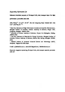
S4. The ratio of the different buoyancy terms under different environmental conditions The vertical integral of the buoyancy- the CAPE - can be divided into three separate terms: thermal, virtual, and water loading (CAPE=CAPE_T+CAPE_V+CAPE_W): 𝑇′
𝐶𝐴𝑃𝐸_𝑇 = ∫ 𝐵𝑇 = 𝑔 ∫ 𝑇 𝑑𝑧 (eq. S1) 0
𝐶𝐴𝑃𝐸_𝑉 = ∫ 𝐵𝑉 = 𝑔 ∫ 0. 61𝑞𝑉′ 𝑑𝑧 (eq. S2) 𝐶𝐴𝑃𝐸𝑊 = ∫ 𝐵𝑊 = −𝑔 ∫ 𝑞𝑊 𝑑𝑧 (eq. S3) In Fig. S5, the CAPE_T and CAPE_V components (calculated according to eqs. S1 and S2) are examined for a large range of environmental conditions: temperature lapse rate between 3 and 8°C/km and cloudy layer RH between 50% and 95%. For these calculations we used the pseudo-adiabatic parcel theory (assuming an immediate removal of the water loading from the parcel, CAPE_W = 0, and that the pressure of the air parcel equals to that of the environment). The pressure and temperature at the lifted condensation level (LCL – representing the cloud base) are set to 900 mb and 17°C. Each subplot represents a different cloud depth: 250, 500, 1500 and 3000 m. Four subspaces represent the four possible states of CAPE_T and CAPE_V (see Fig. S5C for the numbers): (1) no cloud formation, for which the total CAPE < 0 (in blue), (2) total CAPE > 0 driven by CAPE_V > 0 while CAPE_T < 0 (light blue), (3) total CAPE > 0 in which both terms are positive but CAPE_V > CAPE_T (yellow), (4) total CAPE > 0 in which both terms are positive but CAPE_V < CAPE_T (red).
Figure S5. CAPE dependence on environmental temperature lapse rate and RH. Dark-blue areas (1) represent negative CAPE, in which clouds cannot develop. Light-blue areas (2) represent clouds with CAPE_T0. Yellow areas (3) represent clouds with CAPE_T > 0, CAPE_V > 0, and CAPE_T < CAPE_V, while red areas (4) represent clouds with CAPE_T > CAPE_V. Each subplot is for a different cloud depth: (A) 250 m, (B) 500 m, (C) 1500 m, (D) 3000 m.
For all cases in which the parcel forms a cloud (positive CAPE – subspaces 2, 3 and 4), CAPE_V is positive. BV is proportional to the difference in water vapor mixing ratio between the saturated parcel and its environment. Figure S5 demonstrates how the relative importance of the CAPE components changes with cloud depth. The most humid profiles with the lowest temperature lapse rate (most stable) do not support cloud formation (subspace 1) for all the examined cloud depths. The area of this subspace increases with cloud depth due to the increase in the negative contribution of CAPE_T in a stable environment. Changing the pressure or temperature at the LCL would change the moist adiabatic lapse rate (see equation 2 in the main text) and would shift the boundary between subspace 2 (parcel colder than the environment) and subspaces 3 and 4 (parcel warmer than the environment, see Figs. S6 and S7 for examples presenting different
LCL characteristics). As the temperature decreases, representing higher levels in the atmosphere, the moist adiabatic lapse rate increases; thus, for a given environmental lapse rate, clouds that are initially warmer than the environment can become colder if they develop to a sufficient depth. For temperature lapse rates in which CAPE_T > 0 (subspaces 3 and 4), CAPE_T is larger than CAPE_V for deeper clouds. For temperature lapse rates in which CAPE_T < 0 (subspaces 1 and 2), an increase in cloud depth increases the negative value of CAPE_T until it becomes larger (in absolute value) than CAPE_V and inhibits further cloud development. In deep warm convective clouds (Fig. S5D), the space is dominated by two main subspaces: no cloud formation and clouds dominated by CAPE_T. To a first approximation, for cases when CAPE_T > 0, CAPE_V is still likely to be more important for small clouds and its contribution to the total CAPE is inversely proportional to the size of the cloud. This can be explained by two main reasons: 1) A positive lapse rate difference between the cloud and the environment dictates larger temperature differences with increasing distance above the LCL, i.e., CAPE_T has more of a cumulative behavior. 2) On the same note, for a given environmental RH, the differences in water vapor mixing ratio between the (saturated) cloud and the environment are larger at higher temperatures i.e. just above the LCL. This can be generalized for the case of a relatively deep, warm convective cloud in which BT is dominant in the upper part of the cloud but BV is dominant in the lower part. This also means that at the first stage of the cloud evolution, BV dominates, even for cases in which BT later becomes the dominant term. For example, for an environmental temperature lapse rate of 6ºC/km and RH = 80% in the lower part of the cloud (250 m), the CAPE_V to CAPE_T ratio is 1.87, while in the upper part of the cloud (3000 m), it is 0.21. Changing the pressure or temperature at the LCL changes the moist adiabatic lapse rate (see eq. 2 in the main text) and thus shifts the boundary between subspaces 1 and 2 (negative thermal buoyancy) to subspaces 3 and 4 (positive thermal buoyancy) as can be seen in Figs. S6 and S7.
Figure S6. As in Fig. S5 but with LCL temperature of 10°C and pressure of 850 mb.
Figure S7. As Fig. S5 but with LCL temperature of 25°C and pressure of 950 mb.
To include the water loading effect on the buoyancy, we conducted the same calculation as in Fig. S5 using reversible thermodynamic theory (i.e. the parcel maintains the liquid water that is being condensed) rather than the pseudo-adiabatic thermodynamic assumption (in which the condensate sediments out immediately). Figure S8 presents calculations of the CAPE in spaces of environmental temperature lapse rate and RH.
Figure S8. Same as Fig. S5 (with LCL temperature of 17°C and pressure of 900 mb) but with the inclusion of water loading.
S5. Simulations with fixed water vapor contrast between the cloud and its environment To further examine the role of the increased contrast in moisture content between the cloud and its environment (Δqv) we conduct additional set of simulations in which we use the same temperature profiles but with similar Δqv as in the control simulation (see. Fig S9 below).
Figure S9. Vertical profiles of the: a) moisture content contrast between the cloud (at saturation) and the environment (Δqv), b) relative humidity (RH), and c) temperature (T). In b) and c) green, black and blue curves represent the control, +4°c and -4°c simulations, respectively.
Figure S10 presents the temporal evolution of the cloud-mean thermal buoyancy term (BT), virtual term (BV), water loading term (BW), and total buoyancy for all simulations in which Δqv is kept constant (as in the control simulation). This information is complimentary to Fig. 4 (in the main text) that presents the differences between these terms and the control simulation for highlighting the differences between the simulations.
Figure S10. Same as figure S3 but for constant water vapor content contrast between the cloud (at saturation) and the environment (Δqv) rather than fixed RH conditions.
In order to demonstrate that the increase in the vortical circulation (and entrainment rate) with warming in the original set of simulations (as demonstrated by the increase in the horizontal buoyancy gradient - Fig. S4 above) is caused by the increased contrast in moisture content we conduct the same calculation as presented in Fig. S4 to the set of the simulations with constant Δqv. It demonstrates that under constant Δqv conditions the horizontal buoyancy gradient (Fig. S11) does not increase monotonically with temperature as shown for the original set of simulations.
Figure S11. Same as figure S4 but for constant water vapor content contrast between the cloud (at saturation) and the environment (Δqv) rather than fixed RH conditions.
S6. Sensitivity study of changes in the relative humidity with warming We conducted additional simulations with small changes (5%) in the RH, in order to explore the sensitivity of our results. To do so, we have conducted additional simulations with a uniform warming of 4ºC and with 5% increase or decrease in the RH (RH= 75% and 65%, respectively, compared to 70% in the original simulations). This sensitivity study demonstrates that a reduction in the RH with warming results in lower BT (see Figs. S12a and S13a) and higher BV (see Fig. S12b and S13b). These results represent strengthening of the mechanism proposed here due to the larger Δqv that results from the decreased RH. However, increasing the RH (as was also shown in Fig. 4 in the main text) reduces the cooling effect of the cloud with the environmental warming (increasing BT) and reduces the BV contribution due to the decrease in Δqv.
Figure S12. a) thermal buoyancy term, b) virtual term, c) water loading term, and d) total buoyancy as a function of time for different initialization profiles representing uniform temperature increase compared to the control profile but under different RH conditions.
Figure S13. The evolution of the differences from the reference simulation of: (a) thermal buoyancy term (b) virtual term, (c) water-loading term, and (d) total buoyancy, for different initialization profiles representing uniform temperature increase compared to the control profile but under different RH conditions (the simulations that are presented in Fig. S12 above).
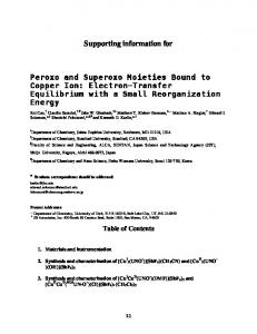
Figure S14 presents a calculation of the required increase in RH for maintaining a constant Δqv, as a function of the initial temperature and the amount of warming. It demonstrates that the increase in RH needed to maintain a constant Δqv is of the order of 1-10% for the initial temperatures that are relevant for warm convective clouds (10-30ºC) and the relevant temperature change (1-5 ºC).
Figure S14. the magnitude of increase in RH (as a function of the initial temperature (X-axis) and the warming (Y-axis)) that is required for maintaining a constant Δqv (water vapor contrast between the cloud and its environment).
References DAGAN, G., KOREN, I. & ALTARATZ, O. 2015. Competition between core and peripherybased processes in warm convective clouds–from invigoration to suppression. Atmospheric Chemistry and Physics, 15, 2749-2760. GARSTANG, M. & BETTS, A. K. 1974. A review of the tropical boundary layer and cumulus convection: Structure, parameterization, and modeling. Bulletin of the American Meteorological Society, 55, 1195-1205.
JAENICKE, R. 1988, Aerosol physics and chemistry, in Meterology LandoltBörnstein, New Ser., vol. 4b, edited by G. Fischer, pp. 391–457,Springer, Berlin. JIANG, H., XUE, H., TELLER, A., FEINGOLD, G. & LEVIN, Z. 2006. Aerosol effects on the lifetime of shallow cumulus. Geophysical Research Letters, 33. MALKUS, J. S. 1958. On the structure of the trade wind moist layer. REISIN, T., LEVIN, Z. & TZIVION, S. 1996. Rain Production in Convective Clouds As Simulated in an Axisymmetric Model with Detailed Microphysics. Part I: Description of the Model. Journal of the Atmospheric Sciences, 53, 497-519. SMALL, J. D., CHUANG, P. Y., FEINGOLD, G. & JIANG, H. 2009. Can aerosol decrease cloud lifetime? Geophysical Research Letters, 36. TZIVION, S., FEINGOLD, G. & LEVIN, Z. 1987. An efficient numerical solution to the stochastic collection equation. Journal of the atmospheric sciences, 44, 3139-3149.
TZIVION, S., REISIN, T. & LEVIN, Z. 1994. Numerical simulation of hygroscopic seeding in a convective cloud. Journal of Applied Meteorology, 33, 252-267. ZHAO, M. & AUSTIN, P. H. 2005. Life cycle of numerically simulated shallow cumulus clouds. Part II: Mixing dynamics. Journal of the Atmospheric Sciences, 62, 12911310.