Supporting Information Quantifying reversible surface ...

Supporting Information Quantifying reversible surface binding via surface-integrated FCS Jonas Mücksch1,3, Philipp Blumhardt1,3, Maximilian T. Strauss1,2, Eugene P. Petrov1,2, Ralf Jungmann1,2 and Petra Schwille1, *

1 Max

Planck Institute of Biochemistry, Martinsried, Germany.

2 Ludwig 3 These

*

Maximilian University, Munich, Germany.

authors contributed equally to this work.

Corresponding author, E-mail: [email protected], Phone: +49 8985782900

Contents

Supplementary Methods ............................................................................................................................... 2 Supplementary Theoretical Basis .................................................................................................................. 5 Supplementary Tables ................................................................................................................................... 8 Supplementary Figures.................................................................................................................................. 9 Supporting References ................................................................................................................................ 22

S1

Supplementary Methods Optical setup

Fluorescence images were recorded on a home-built custom-type TIRF microscope, which was constructed around a Nikon Ti-S microscope body with oil immersion objective (Nikon SR Apo TIRF, 100x magnification, 1.49 numerical aperture (NA)). Custom-built excitation and detection pathways (Supplementary Fig. S8) extended the commercial body. Four laser lines (490 nm (Cobolt Calypso, 50 mW nominal), 532 nm (Cobolt Samba, 100 mW nominal), 561 nm (Cobolt Jive, 50 mW nominal) and 640 nm (Cobolt 06-MLD, 140 mW nominal)) were attenuated with an acousto-optical tunable filter (Gooch & Housego TF-525-250), which was interfaced through a PCI Express card (PCIe-6323 and BNC-2110) and controlled with a home-written LabView 2011 software (all National Instruments, Austin, USA). A polarization-maintaining single-mode fiber (kineFLEX-P-3-S-405.640-0.7-FCS-P0 and kineMATIX, Qioptiq, Hamble, UK) spatially filtered the excitation beams. At the fiber exit, the beam was collimated by an achromatic lens (f=25 mm, Edmund Optics, Karlsruhe, Germany) and the polarization refiltered through a polarizing beam splitter (CCM1PBS251/M, Thorlabs, Dachau. Germany). Achromatic doublets were employed for three-fold beam expansion (f = -25, 75 mm) and focusing the excitation in the objective’s back focal plane (f = 225 mm, all purchased from Edmund Optics, Karlsruhe, Germany). A four-color notch beam splitter

(zt405/488/561/640rpc flat, AHF Analysentechnik, Tübingen, Germany) directed the excitation laser beams towards the objective. A piezo-electric stage (Q545, Physikalische Instrumente, Karlsruhe, Germany) translated the excitation beam off-axis to switch between wide-field, HILO or TIRF imaging. The emission light was directed towards the microscope side-port and spectrally bandpass filtered (Semrock BrightLine 593/46, AHF Analysentechnik, Tübingen, Germany) in infinity space. The detection pathway comprised a 4f telescope (f = 200 mm, AC254-200-A-ML, Thorlabs, Dachau, Germany) and an electron-multiplying charge-coupled device (EMCCD) camera (iXon Ultra 897, Andor Technologies, Belfast, UK). The camera acquisition triggered the transmission of the acousto-optical tunable filter by TTL pulses. Images were recorded using the Andor Solis software (Andor Technologies, Version 4.28). A custom-built focus stabilization eliminated the drift of the focus position: A near infrared laser (LP785SF20, Thorlabs, Dachau, Germany) was back-reflected from the sample in TIRF configuration and focused on a CMOS camera (UI-3240CP-NIR-GL, Imaging Development Systems, Obersulm, Germany). A feedback control implemented in LabVIEW 2015 (National Instruments, Austin, USA) maximized the crosscorrelation of the images of the laser spot and a reference image, respectively. The axial sample position was adjusted every 200 ms accordingly (P737.2SL and E-709.SRG, Physikalische Instrumente, Karlsruhe, Germany) to keep the sample in focus.

SI-FCS image acquisition

Unless stated otherwise, SI-FCS analysis was performed on image sequences of 64x64 pixel (4x4 binning) and for comparable analysis resized to the camera resolution of 256x256 pixels. Image stacks were recorded for 1.5 million frames for 7 nt, 8 nt and 9 nt, and 150,000 frames for 10 nt, respectively. The exposure time was 10 ms and the camera frame rate 85 Hz for 7 nt, 8 nt, 9 nt, or 10 Hz 10 nt. The EM gain setting was varied, but does not influence the kinetics (data not shown). To exclude any effect of the EM gain, we varied this parameter systematically in an initial set of experiments, but observed no influence on the autocorrelation decay times obtained from SI-FCS measurements (data not shown). S2

SI-FCS data analysis

The autocorrelation curves were computed and analyzed using a custom-written Matlab 2017a (The MathWorks, Natick, USA) software: Each image was subdivided into 7X7 ROIs, each of them covering 31X31 pixels, spaced in a grid around the center of illumination. The effect of the choice of ROI size is discussed in Supplementary Fig. S11. The signal in each ROI was integrated, yielding 49 intensity traces, which were bleach and drift-corrected by a single exponential, and individually correlated using the multiple-τ algorithm1, in which we doubled the bin width after every sixteenth point in the autocorrelation curve. The obtained autocorrelation curves were fitted individually by a single exponential decay with an offset, from which the amplitude and the characteristic decay time were obtained. For samples containing two species, the autocorrelation curves were fitted by a sum of two exponentials with an offset. In the titration experiments, the biexponential fit accounted for a supposedly non-specific component appearing at high concentrations (10 nM for 10 nt, 100 nM for 9 nt).

Monte Carlo Simulations of SI-FCS measurements

If not mentioned otherwise, Monte Carlo Simulations were performed using a home-written MATLAB code (R2016a, MathWorks). The time step between two iterations was set to 𝑑𝑑𝑑𝑑 = 1 ms and the signal from 10 iterations was integrated to form one time point in the signal trace. This corresponds to a time resolution of the detector of 10 ms. For these simulations, we only considered fluctuations in signal originating from binding and unbinding events. Therefore, we initialized 𝑁𝑁surf immobile binding sites at a surface and had a fraction 𝛽𝛽 =

1+

1

𝑘𝑘𝑑𝑑 𝑘𝑘𝑎𝑎

of them initially occupied. Moreover, we defined a probability of binding 𝑃𝑃binding =

1 − 𝑒𝑒 −𝑘𝑘𝑎𝑎 𝑑𝑑𝑑𝑑 and unbinding 𝑃𝑃unbinding = 1 − 𝑒𝑒 −𝑘𝑘𝑑𝑑 𝑑𝑑𝑑𝑑 . During each iteration, we treat occupied and unoccupied binding sites differently. For all bound sites we generated a uniformly distributed random number in the interval (0,1). If the random number was smaller than a threshold given by 𝑃𝑃unbinding, the binding site was converted to an unoccupied state, otherwise it remained unchanged. The transitions from the unbound to bound state were simulated following an equivalent strategy. Each bound receptor contributed with the brightness 1 to the signal per iteration, each unoccupied binding site did not contribute to the signal. The described code does not simulate images, but only the integrated signal over a simulated area. Although it is straightforward to add the functionality of simulating images, all simulations with varying surface density (supplementary figure S6) were performed using the previously published Picasso tool2.

Fluorescently labeled complementary ssDNA in solution

Labeled imager strands with the sequence 5’-CTAGATGTAT-3’-Cy3B were purchased from Eurofins Genomics.

Buffers

For simplicity, we name the used buffers A+ and B+. Buffer A+ contains 10 mM Tris-HCl, 100 mM NaCl, 0.05 v% Tween20 and is adjusted to pH 8. Buffer B+ contains 5 mM Tris-HCl, 10 mM MgCl2, 1 mM EDTA, 0.05 v% Tween20 and is adjusted to pH 8.

Preparation of DNA origami samples

DNA origami structures were synthesized as previously described2. In brief, structures were folded in a one-pot reaction with 40 µl total volume containing 10 nM scaffold (M13mp18), 10 nM biotinylated staples for surface attachment, 100 nM core staples and 1 µM extended staples in 1xTE buffer supplemented with 12.5 mM MgCl2. Structures were folded by first holding for 5 min at 80 °C, then going from 65 °C to 4 °C S3

over the course of 3 hours. The assembly of the DNA origami structures was confirmed by super-resolution imaging with DNA-PAINT (see Supplementary Fig. S9).

Assembly of the Sample Chamber

Surfaces with immobilized DNA origami structures were prepared following a previously reported protocol2. In brief, high precision #1.5 coverslips (Paul Marienfeld GmbH, Germany) were sonicated in acetone (chemical grade, Merck KGaA, Germany) for 10 minutes and then rinsed twice with ethanol (chemical grade, Merck Millipore, Germany) and water (milli-Q, Merck Millipore, Germany) and gently dried with pressurized air. The cleaning of the coverslip was completed by putting a drop of 2-propanol on it (Uvasol, Merck KGaA, Germany) and wiping with a paper tissue (Kimtech Science, Sigma Aldrich, Germany). The same procedure was performed on microscope slides (76x26 mm², Menzel, Germany). The high precision coverslip and the microscope slide were assembled into a flow chamber by gluing them together with double-sided sticky-tape (Scotch, Conrad Electronic SE, Germany), yielding a roughly 5x22x0.08 mm3 large chamber. In a series of volume exchanges, the flow chamber was first incubated with 20 µl of 1 mg/ml albumin, biotin-labeled bovine (Sigma-Aldrich) in buffer A+ for two minutes, washed with 40 µl buffer A+, incubated with 20 µl of 0.5 mg/ml streptavidin (Thermo Fisher Scientific) in buffer A+ for two minutes, washed with 40 µl buffer A+, washed with 40 µl buffer B+, incubated with 20 µl of 0.5 nM of the desired folded DNA origami structures, which were dissolved in buffer B+, for ten minutes, washed with 40 µl buffer B+ and finally loaded with 20 µl of imager strand in the required concentration. In a final step, the chamber was sealed using two-component epoxy glue (Toolcraft, Conrad Electronic SE, Germany). We verified the final concentration of fluorescently labeled ssDNA by confocal FCS measurements (see Supplementary Fig. S10).

S4

Supplementary Theoretical Basis Theoretical Model for the Autocorrelation Function of a One-Component BindingUnbinding Reaction without Diffusion

Considerable effort has been previously put into the derivation or approximation of an all-embracing correlation curve, which covers lateral 2D-diffusion, 3D diffusion and reversible binding3–6. To reduce the complexity, and as we are mainly interested in the measurement of binding kinetics, we pursue a simplified approach. We define the autocorrelation function 𝐺𝐺𝑚𝑚𝑚𝑚𝑚𝑚𝑚𝑚 , which is directly computed from acquired images, as 𝐺𝐺𝑚𝑚𝑚𝑚𝑚𝑚𝑚𝑚 (𝜏𝜏) =

〈𝛿𝛿𝐹𝐹(0)𝛿𝛿𝛿𝛿(𝜏𝜏)〉 〈𝐹𝐹〉2

(1)

Here, 𝐹𝐹 is the fluorescence signal, which can be decomposed into a correlated contribution 𝐹𝐹𝑐𝑐 (𝑡𝑡) and an uncorrelated background 𝐵𝐵𝑔𝑔 (𝑡𝑡). In a typical equilibrium system, the total fluorescence signal can be expressed in terms of its mean 〈𝐹𝐹〉 and the fluctuations 𝛿𝛿𝛿𝛿(𝑡𝑡) around this mean: 𝐹𝐹(𝑡𝑡) = 〈𝐹𝐹〉 + 𝛿𝛿𝛿𝛿(𝑡𝑡) = 〈𝐹𝐹𝑐𝑐 〉 + 〈𝐵𝐵𝑔𝑔 〉 + 𝛿𝛿𝐹𝐹𝑐𝑐 (𝑡𝑡) + 𝛿𝛿𝐵𝐵𝑔𝑔 (𝑡𝑡) (2)

Provided that 𝐵𝐵𝑔𝑔 (𝑡𝑡) is uncorrelated background, the computed autocorrelation function reduces to: 𝐺𝐺𝑚𝑚𝑚𝑚𝑚𝑚𝑚𝑚 (𝜏𝜏) =

〈𝛿𝛿𝐹𝐹𝑐𝑐 (0)𝛿𝛿𝐹𝐹𝑐𝑐 (𝜏𝜏)〉

(3)

2

�〈𝐹𝐹𝑐𝑐 〉+〈𝐵𝐵𝑔𝑔 〉�

Practically, it is rather relevant to measure the correlation curve 𝐺𝐺𝑐𝑐 (𝜏𝜏) based on 𝛿𝛿𝐹𝐹𝑐𝑐 (𝜏𝜏) and normalize to the mean of 𝐹𝐹𝑐𝑐 (𝜏𝜏). Provided that the background can be measured in a separate blank control sample, 𝐺𝐺𝑐𝑐 (𝜏𝜏) can be calculated easily7: 𝐺𝐺𝑐𝑐 (𝜏𝜏) = 𝐺𝐺𝑚𝑚𝑚𝑚𝑚𝑚𝑚𝑚 (𝜏𝜏)

〈𝐹𝐹〉2

2

�〈𝐹𝐹〉−〈𝐵𝐵𝑔𝑔 〉�

(4)

It is worth noting that the amplitude of the autocorrelation curve is decreased by uncorrelated background, but the temporal decay is not altered. In the context of the SI-FCS measurements presented here, the uncorrelated background can be not only background noise or stray light, but also the signal contribution from freely diffusing ligand. The latter can be considered as uncorrelated background if the 3D diffusion of labeled ligand through the detection volume is occurring on a much shorter timescale than the considered binding kinetics. To obtain an expression for 𝐺𝐺𝑐𝑐 (𝜏𝜏), we note that the fluorescence signal fluctuations have a contribution from freely diffusing and from bound ligand 𝛿𝛿𝐹𝐹𝑐𝑐 ~𝛿𝛿𝛿𝛿 + 𝛿𝛿𝛿𝛿. As discussed above, only the latter is correlated on the considered timescale. Analogously, we note that 〈𝐹𝐹𝑐𝑐 〉~〈𝐶𝐶〉. Following the common scheme of derivations for FCS, we assume equivalence of the time and ensemble averages and rewrite 𝐺𝐺𝑐𝑐 (𝜏𝜏) as follows: 𝐺𝐺𝑐𝑐 (𝜏𝜏) =

∫ 𝑑𝑑 3 𝑟𝑟 ∫ 𝑑𝑑 3 𝑟𝑟 ′ Φ𝐶𝐶𝐶𝐶 (𝜏𝜏) 𝛿𝛿(𝑟𝑟−𝑟𝑟 ′ ) 〈𝐶𝐶〉2 (∫ d3 𝑟𝑟)²

(5)

S5

Here, the integrals run over the entire detection volume. To make use of equation 5, we aim to find an expression for 𝛿𝛿𝛿𝛿, or the concentration correlation function

Φ𝐶𝐶𝐶𝐶 (𝜏𝜏) = 〈𝛿𝛿𝛿𝛿(0)𝛿𝛿𝛿𝛿(𝜏𝜏)〉

(6)

The fluctuations in C are governed by binding kinetics, which we assume to be a simple bimolecular reaction of the type A + B ⇌ C, where A is a ligand, freely diffusing above a surface, B is an unbound receptor, which is immobilized at a surface, and C is the bound receptor-ligand-pair (see Fig. 1a). Under the assumption that all diffusion dynamics through a considered region of interest are equilibrated, the change of the concentration of conjugates 𝐶𝐶, will be governed by a source and a sink term:

d𝐶𝐶 d𝑡𝑡

= 𝑘𝑘𝑎𝑎 𝐴𝐴𝐴𝐴 − 𝑘𝑘𝑑𝑑 𝐶𝐶

(7)

Here, we introduced the association rate 𝑘𝑘𝑎𝑎 and the dissociation rate 𝑘𝑘𝑑𝑑 . Both rates fulfill the well-known relation to the dissociation constant 𝐾𝐾𝑑𝑑 and the mean concentrations: 𝑘𝑘

〈𝐴𝐴〉〈𝐵𝐵〉 〈𝐶𝐶〉

𝐾𝐾𝑑𝑑 = 𝑘𝑘𝑑𝑑 = 𝑎𝑎

(8)

As the total number of surface receptors 𝑆𝑆 = 〈𝐵𝐵〉 + 〈𝐶𝐶〉 = const is constant, it is evident that a decrease of receptor-ligand pairs will result in an increase of free receptor by the same magnitude: 𝛿𝛿𝛿𝛿 = −𝛿𝛿𝛿𝛿. Therefore, the differential equation for 𝐶𝐶 is easily transformed into a differential equation for Φ𝐶𝐶𝐶𝐶 : dΦ𝐶𝐶𝐶𝐶 (𝜏𝜏) d𝜏𝜏

= −(𝑘𝑘𝑎𝑎 〈𝐴𝐴〉 + 𝑘𝑘𝑑𝑑 )Φ𝐶𝐶𝐶𝐶 (𝜏𝜏)

(9)

Differential equations of this kind are very well known and have the simple solution Φ𝐶𝐶𝐶𝐶 (𝜏𝜏) = Φ0 𝑒𝑒 −𝜏𝜏/𝜏𝜏𝑐𝑐

(10)

The obtained exponential function decays with the characteristic time constant −1

𝜏𝜏𝑐𝑐 = (𝑘𝑘𝑎𝑎 〈𝐴𝐴〉 + 𝑘𝑘𝑑𝑑 )−1 = �𝜏𝜏𝑎𝑎−1 + 𝜏𝜏𝑑𝑑−1 � , which is related to the dwell time 𝜏𝜏𝑑𝑑 = 𝑘𝑘𝑑𝑑−1 and the association time 𝜏𝜏𝑎𝑎 = (𝑘𝑘𝑎𝑎 〈𝐴𝐴〉)−1.

To obtain an expression for Φ0 , we follow the argumentation of Thompson and colleagues3: First, Φ0 needs to meet the initial condition Φ𝐶𝐶𝐶𝐶 (𝜏𝜏 = 0) = Φ0 = 〈𝛿𝛿𝐶𝐶 2 〉. This quantity is known as the variance. To find the underlying distribution, we note that for every given point in time, each surface receptor occupies one out of two states: bound to a ligand or unbound. Provided that all receptors are independent, this corresponds to a binomial distribution, which has the variance Φ0 = 𝑆𝑆𝑆𝑆(1 − 𝛽𝛽). Here we used again the total surface concentration of receptors 𝑆𝑆 = 〈𝐵𝐵〉 + 〈𝐶𝐶〉, and introduced the fraction of bound receptors 〈𝐶𝐶〉

𝛽𝛽 = 〈𝐵𝐵〉+〈𝐶𝐶〉 =

1

𝑘𝑘𝑑𝑑 1+ 〈𝐴𝐴〉 𝑘𝑘𝑎𝑎

𝜏𝜏

= 𝜏𝜏 𝑐𝑐 , which can be interpreted as the success probability of the binomial distribution. 𝑎𝑎

〈𝐵𝐵〉

Analogously, the fraction of unoccupied receptors reads (1 − 𝛽𝛽) = 〈𝐵𝐵〉+〈𝐶𝐶〉 =

obtain

𝜏𝜏

Φ0 = 〈𝐶𝐶〉 𝜏𝜏 𝑐𝑐 = 〈𝐶𝐶〉(1 − 𝛽𝛽) 𝑑𝑑

1

𝑘𝑘 〈𝐴𝐴〉 1+ 𝑎𝑎 𝑘𝑘𝑑𝑑

𝜏𝜏

= 𝜏𝜏 𝑐𝑐 . Therefore, we 𝑑𝑑

(11)

And finally, after insertion into equation 5, we get an analytic expression for the autocorrelation function of reversible binding: S6

𝐺𝐺𝑐𝑐 (𝜏𝜏) =

1 𝜏𝜏𝑐𝑐 −𝜏𝜏/𝜏𝜏 𝑐𝑐 𝑒𝑒 𝑁𝑁𝐶𝐶 𝜏𝜏𝑑𝑑

=

1 1−𝛽𝛽 −𝜏𝜏/𝜏𝜏 𝑐𝑐 𝑒𝑒 𝑁𝑁𝑆𝑆 𝛽𝛽

(12)

Here, we introduced the average number of bound receptors 𝑁𝑁𝑐𝑐 and the total number of receptors 𝑁𝑁𝑆𝑆 in the detection volume. Alternatively, equation 12 can be obtained as a limiting case of the advanced derivation of the full autocorrelation by Thompson and colleagues3. Interestingly, the amplitude 𝐺𝐺0 = lim 𝐺𝐺𝐶𝐶 (𝜏𝜏) of the correlation is not only proportional to the absolute number of occupied binding sites, but 𝜏𝜏→0

also depends on the fraction of unoccupied sites. However, if 𝜏𝜏𝑎𝑎 ≫ 𝜏𝜏𝑑𝑑 , i.e. in case of low concentration of labeled ligand 〈𝐴𝐴〉 ≪ 𝐾𝐾𝑑𝑑 , the number of occupied binding sites can be obtained directly as the inverse of the correlation amplitude.

S7

Supplementary Tables Free energy of DNA hybridization sequence

5’-TTATACATC-3’ 5’-TTATACATCT-3’ 5’-TTATACATCTA-3’ 5’-TTATACATCTAG-3’

concent overlap ration 〈𝑨𝑨〉[𝐧𝐧𝐧𝐧] 10

7 nt

10

9 nt

10

8 nt

1

10 nt

predicted 𝚫𝚫𝚫𝚫

𝐤𝐤𝐤𝐤 �𝐦𝐦𝐦𝐦𝐦𝐦�

measured 𝝉𝝉𝒄𝒄 [𝐬𝐬]

36.03

0.44 ± 0.01

41.98

4.86 ± 0.05

37.83 48.98

measured 𝒌𝒌𝒅𝒅 [𝐬𝐬 −𝟏𝟏 ]

2.272 ± 0.052

2.39 ± 0.05 90 ± 7

estimated 𝒌𝒌𝒂𝒂 ∙ 𝟏𝟏𝟏𝟏−𝟔𝟔 [𝐌𝐌 −𝟏𝟏 𝐬𝐬−𝟏𝟏 ]

0.418 ± 0.009 0.206 ± 0.002

0.0111 ± 0.0009

5.15 ± 0.12 1.97 ± 0.04 5.23 ± 0.05 4.84 ± 0.39

Table S1. Hybridization parameters for different DNA sequences with the target sequence 5‘CTAGATGTAT-3’. SI-FCS measurements were performed in a low concentration regime of labeled strands, such that the dissociation rate is directly estimated from the characteristic decay time of the 〈𝐴𝐴〉 ≪ 𝐾𝐾

autocorrelation curve 𝜏𝜏𝑐𝑐 �⎯⎯⎯� 𝜏𝜏𝑑𝑑 = 𝑘𝑘−1 𝑑𝑑 . For each pair of sequences, the free energy Δ𝐺𝐺 of hybridization was estimated using the Nucleic Acid Package (NUPACK)8 with the following settings: temperature 𝑇𝑇 = 296.15 K, concentration of Na+ 50 mM, concentration of Mg2+ 9 mM. The calculations were performed based on the parameters provided by SantaLucia9, which had to be adjusted for our buffer conditions. To describe our conditions best, we used the minimum concentration of Na+ compatible with ref. 9, which compensates partially for the Tris in our buffer. The remaining Na+ could be accounted for by lowering the Mg2+, although the relevant equivalent amount of Mg2+ would be small10–12. The dissociation constant 𝐾𝐾 and the binding free energy Δ𝐺𝐺 are linked via the well-known equation Δ𝐺𝐺 = −𝑅𝑅𝑅𝑅 ln

𝐾𝐾 . 𝐾𝐾0

Here, we

introduced the gas constant R, the temperature T, and a reference constant 𝐾𝐾0 = 1 M, which has the sole purpose to ensure that the logarithm is applied to a dimensionless quantity. Consequently, after obtaining 𝑘𝑘

Δ𝐺𝐺

𝑘𝑘𝑑𝑑 as the inverse of 𝜏𝜏𝑐𝑐 , the association rate is calculated as 𝑘𝑘𝑎𝑎 = 𝑑𝑑 𝑒𝑒 𝑅𝑅𝑅𝑅 . The obtained association rates 𝐾𝐾 0

can be regarded as estimates of the true rates. The estimated association rates are in line with values reported elsewhere13–17. Moreover, all estimated association rates appear to be similar, regardless of the basepair overlap. The same observation was recently reported for 9 nt and 10 nt hybridization15.

S8

Supplementary Figures Control for photobleaching

Figure S1. Dependence on Excitation Power. a) Bleaching is observed as an apparent reduction of the residence time and therefore also as a reduction of 𝜏𝜏𝑐𝑐 . The autocorrelations were averaged over several ROIs and measured with 〈𝐴𝐴〉 = 10 nM and 9 nt base pair overlap. We identified irradiances below 𝐼𝐼0 < 0.037

kW cm2

to be free from bleaching. For 10 nt the residence times are significantly longer and the

bleaching free regime was determined to be 𝐼𝐼0 < 1.6 ∙ 10−3

kW , cm2

which was achieved by reducing the

excitation power and the frame rate of acquisition from 85 Hz to 10 Hz (data not shown). b) The Gaussian shape of the illumination profile may induce a spatial profile of the 𝜏𝜏𝑐𝑐 obtained from different ROIs. For high irradiances, the apparent diffusion time is not only globally lowered due to bleaching, but also is shortest in the center of illumination. For irradiances below 𝐼𝐼0 < 0.037 becomes negligible.

S9

kW , cm2

this spatial distribution

Reproducibility of SI-FCS measurements

Figure S2. Reproducibility of SI-FCS measurements. To estimate the robustness and reproducibility of this method, we repeated identical measurements on one and the same sample. When superimposing the autocorrelation curves from seven measurements on the hybridization of ssDNA with 9 nt overlap, all curves were indistinguishable (Fig. S2a). For every measurement, the standard deviation of the characteristic decay times obtained from 49 ROIs was considerably lower than 10% of the mean, demonstrating that consistent results are obtained over the entire field of view, independent of the local illumination profile. Moreover, the comparison of the average characteristic decay times from several independent measurements (Fig. S2b) showed that the scatter is less than 5% of the overall average, that is 〈𝜏𝜏𝑐𝑐 〉 = 4.81 ± 0.05) 𝑠𝑠, with the error being the standard deviation of the seven measurements. This series of similar measurements demonstrated the excellent accuracy of SI-FCS for the determination of binding rates.

S10

Determination of kinetic rates from two measurements

Figure S3. Extraction of association and dissociation rates from two measurements. Based on equation 1 (main text) the knowledge of two points of the titration curve is in principle sufficient to determine the association rate 𝑘𝑘𝑎𝑎 , the dissociation rate 𝑘𝑘𝑑𝑑 and therefore also the equilibrium constant 𝐾𝐾 = 𝑘𝑘𝑑𝑑 ⁄𝑘𝑘𝑎𝑎 . a) For 9 nt, the full titration curve (left panel), 𝑘𝑘𝑎𝑎 (center panel) and 𝑘𝑘𝑑𝑑 (right panel) calculated from pairs of two measurements along the titration curve. The relative difference �𝑘𝑘𝑎𝑎/𝑑𝑑 − 𝑘𝑘𝑎𝑎/𝑑𝑑,titration ��𝑘𝑘𝑎𝑎/𝑑𝑑,titration is represented by the color of the points. For pairs of concentrations (〈𝐴𝐴1 〉, 〈𝐴𝐴2 〉) of differently dominated regimes (𝑘𝑘𝑑𝑑 ≪ 𝑘𝑘𝑎𝑎 〈𝐴𝐴1 〉 and 𝑘𝑘𝑑𝑑 > 𝑘𝑘𝑎𝑎 〈𝐴𝐴2 〉) the rates can be recovered with an error smaller than 20% (highlighted as squares). Pairs of concentrations which were different less than a factor of two were excluded from the analysis and marked as crosses. Concentration pairs leading to a relative error of more than 100% saturated the color scale and were marked as diamonds. b) Same as panel a), but the analysis was based on data sets from 10 nt hybridizations. S11

Required measurement time

Figure S4. Effect of the measurement time. We performed Monte Carlo simulations to evaluate the effect of the duration of individual measurements. To this end, we simulated 10 signal traces, which were 105 times longer than the characteristic decay time, fitted the resulting autocorrelation curves and related the results to the initially set characteristic decay time. To assess the effect of the measurement time but keep the statistics comparable, we cut the initial traces into shorter traces and repeated the analysis, thereby keeping constant the total number of binding events observed. For example, to analyze the case of traces, which are 103 times longer than the characteristic decay time, we split each of the 10 initial traces (105 times longer than 𝜏𝜏𝑐𝑐,sim ) into 100 sub-traces and subsequently computed and analyzed all resulting 1000 autocorrelation curves. Fig. S4a shows the obtained decay time 𝜏𝜏𝑐𝑐,meas as a function of the duration of individual simulations. Both parameters are normalized to the characteristic decay time 𝜏𝜏𝑐𝑐,sim set in the simulation, which we expect to be the relevant time scale when assessing the required measurement time18,19. To avoid any effects of poor sample statistics, we repeated every simulation 10 times and varied the number of considered binding sites from 1 to 1000. The corresponding results are shown as mean (central line) plus/minus standard deviation of the ten simulations (shaded area). No difference between the different settings is discernible and it appears that the bias from the autocorrelation (biased estimator1,18) converges to zero for sufficiently long measurements. Nonetheless, it should be noted, that the required measurement times for binding studies using SI-FCS can be long. When aiming for a bias smaller than 10%, one should conduct measurements at least 300-fold longer than the characteristic decay time. Therefore, slow dynamics require particularly long measurement time, which makes the use of a S12

focus stabilization system essential. Nonetheless, for a correlation curve originating from binding and unbinding the convergence happens significantly faster than for a correlation curve originating from 2D diffusion (Fig. S4a). The reason is the different shape of the correlation curves. For reversible binding, the autocorrelation curve decays relatively fast as a single exponential 𝐺𝐺𝐶𝐶 (𝜏𝜏)~𝑒𝑒 𝜏𝜏

−1

autocorrelation curve for 2D diffusion 𝐺𝐺2𝐷𝐷 (𝜏𝜏)~ �1 + 𝜏𝜏 � 𝐷𝐷

−

𝜏𝜏 𝜏𝜏𝑐𝑐

, whereas the

has a significantly longer tail. Fig. S4b

demonstrates this effect by superimposing both autocorrelation curves with a time axis normalized to the relevant decay times 𝜏𝜏𝑐𝑐 and 𝜏𝜏𝐷𝐷 respectively.

To confirm the simulation results, we re-analyzed the measurements for 7-10 nt in a similar way as we analyzed the long simulated traces. By this, we can superimpose the simulated dependence from Fig. S4a and the measurement results (Fig. S4c). Strikingly, without any fitting involved, the simulation and the experimental results follow the same trend. Moreover, in this depiction, we see no difference between different nucleotides, which is expected as we normalize by 𝜏𝜏𝑐𝑐 . Nonetheless, we can conclude that the underlying dynamics for 7-10 nt hybridization are identical, and only occur on different time scales, which makes the depicted relation a universal concept. For short measurement times, the bias of the experimental data seems to be slightly larger than the simulation suggests, which we attribute to noise involved in the measurements. From (Fig. S4c) we conclude that the systematic bias on the obtained characteristic decay time cannot be smaller than indicated by the simulated dependence. The bias cannot be reduced below this line, not even by an increasing number of binding events observed within the same measurement duration. The only option to reduce the systematic bias is an increased duration of the total measurement time. Furthermore, Fig. S4c shows that an individual measurement has to be at least 300fold longer than the characteristic decay time to achieve a bias smaller than 10%. Based on this finding, we can replot Fig. S4c without normalization of all times and superimpose a border, which corresponds to the 10% systematic bias (solid line, Fig. S4d). All points on the right hand side of this line have a bias of less than 10%, which gives a direct and quick check for whether a particular measurement was long enough to provide the required accuracy.

S13

SI-FCS measurements of reversible binding are calibration-free

Figure S5. SI-FCS is calibration-free and robust to defocused imaging. The calibration of the detection volume is a crucial step in confocal FCS measurements. On the other hand, camera-based SI-FCS measurements on diffusion dynamics in supported lipid bilayers have been shown to be calibration-free by variable pixel binning during post-processing of images20. In contrast, when looking at the reversible binding of labeled freely diffusing ligand to a surface-immobilized target, SI-FCS is intrinsically calibrationfree, as it does not require any lateral spatial resolution. Here, the signal fluctuation originates from binding and unbinding events to the surface. Any changes in the lateral size of the detection volume do not qualitatively alter the underlying kinetics of the fluctuating signal. To prove this, we performed a series of measurements at different axial positions of the detection volume relative to the sample surface. This is equivalent to systematic defocusing, which varies the lateral size of the PSF. The SI-FCS experiments presented here are within reasonable limits robust to any defocusing of the sample. The situation changes when looking at lateral diffusion through a detection volume, e.g. a region of interest spanning a certain number of pixels on the camera detector. In this case, the decay of the autocorrelation curve depends on the diffusion coefficient, the size of the region of interest and the size of the PSF6,20. a) Autocorrelation curves and single-exponential fits obtained from the same sample but different axial positions of the specimen. The axial positions are color coded and can be inferred from panel b). b) Characteristic decay times obtained from single-exponential fits of the SI-FCS autocorrelation functions measured for different sample positions along the optical axis.

S14

Surface density accessible to SI-FCS

Figure S6. Performance of SI-FCS at different receptor surface densities: Simulations. We simulated SIFCS image series (see Supplementary Theoretical basis) using the Picasso software tool 2. To assess the surface densities of receptors which are compatible with SI-FCS, we started off by simulating SI-FCS measurements for 24X24 pixels (160x160 nm² per pixel), with 𝑘𝑘𝑑𝑑 = 1 s −1, 𝑘𝑘𝑎𝑎 〈𝐴𝐴〉 = 0.008 s −1 , and 3 to 100,000 receptors in the considered area. The simulated frame rate was 10 Hz and a total of 40,000 frames was simulated for each run, corresponding to a total measurement duration 𝑡𝑡meas = 4000 s. Each simulation was performed ten times to develop a feeling for the scatter of results. Fig. S6a-c show ten individual curves each (light grey), superimposed with their mean (blue line) and the corresponding single exponential fit (red line) from which the characteristic decay time is extracted. These curves demonstrate once more that a single exponential describes the autocorrelation curves appropriately. Second, the least from 300 binding sites on, the statistical scatter for the simulated conditions becomes small. Each −1 individual autocorrelation curve represents on average 𝛽𝛽𝑁𝑁𝑆𝑆 �𝑘𝑘𝑑𝑑−1 + 𝑘𝑘𝑎𝑎−1 〈𝐴𝐴〉−1 �𝑡𝑡meas binding events (for S15

𝑁𝑁𝑆𝑆 = 300 less than 104 events). For all receptor densities considered, we recovered the simulated characteristic decay times accurately (Fig. S6d). With reasonable computation times (maximum number of binding sites 105), we could not find a regime where SI-FCS could not recover the simulated characteristic decay times. This is a clear advantage of SI-FCS over tracking based approaches in which the residence time is determined. Here, we are not confined to regimes where individual particles can be identified. Figures S6e show representative simulated images for 300, 3,000 and 30,000 binding sites. Clearly, already in the case of 3,000 binding sites, a tracking based approach would suffer from misassignments during the reconstruction of tracks, leading to overestimations of residence times. We note that the number of binding sites or the surface density of binding sites are not particularly good parameters to compare the performance of SI-FCS and tracking-based estimations of the residence time. As tracking relies on the detection of individual particles, it is rather relevant to replot Fig. S6d in terms of the occupied binding sites per resolution disk 𝑁𝑁𝑏𝑏 = 𝑆𝑆𝑆𝑆𝐴𝐴resolution disk (Fig. S6f). Here, we used the total density of binding sites S, and the fraction of occupied binding sites 𝛽𝛽 =

1+

1

𝑘𝑘𝑑𝑑 𝑘𝑘𝑎𝑎

(see Supplementary

Methods). As the resolution disk we define a circle with the 1/e² value 𝑤𝑤𝑥𝑥𝑥𝑥 of the Gaussian-shaped PSF as radius. This equals to the assumption that two resolution limited spots can be distinguished reliably if their centers are separated by at least 𝑤𝑤𝑥𝑥𝑥𝑥 . As shown in Fig. S6f, the SI-FCS approach reliably reproduces the simulated binding times not only in a regime where tracking-based approaches would perform, but also at surface densities of bound receptors which exceed the tracking regime by at least two orders of magnitude.

S16

Measurements surface density

Figure S7. Performance of SI-FCS at different receptor surface densities: Experimental data a) Autocorrelation curves obtained from five individual SI-FCS measurements of the hybridization kinetics of a 9 nt overlap. The measurements differ in the origami surface density, which is intrinsically difficult to control quantitatively. As a simple approach, we incubated the surfaces for the same time with different concentrations of DNA origami (0.03, 0.1, 0.3, 1.0, and 3 nM). SI-FCS yields reasonably consistent decay times for the range of investigated surface densities, although a slight increase is observed for very high surface densities. The dashed line corresponds to the surface concentration we used in typical SI-FCS measurements (Fig. 2 and 3 from the main text). b) Representative images corresponding to the conditions described in a) For the lowest surface concentrations, particle tracking approaches could be potentially conducted, whereas for origami concentrations above 0.1 nM, tracking approaches would clearly fail, because individual events cannot be identified any longer. SI-FCS yielded smooth low-noise autocorrelation curves even in regimes that were clearly not accessible to tracking approaches. Time series were recorded without binning with a resolution of 256x256 pixel.

S17

TIRF microscope

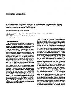
Figure S8. Custom-built TIRF microscope. See supplementary methods.

S18

DNA-PAINT reconstruction of binding sites on DNA origami structures

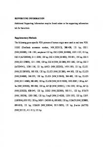
Figure S9. Super-resolution of DNA origami exposing 12 single-stranded DNA handles. A) Schematic of the rectangular DNA origami structures, exposing 12 ssDNA handles. The image was generated with the Picasso software tool.2 b) Representative DNA-PAINT images of the rectangular origamis.

S19

Measurement of the ligand concentration

Figure S10. Direct measurement of the ligand concentration. To validate that the target concentration of ligand is indeed reached in the sample, we performed confocal FCS measurements on a commercial LSM 780 Confocor3 system (Zeiss AG, Oberkochen, Germany). As we were interested in the concentration of imager strand in solution, we positioned the confocal volume 30 µm above the origami-coated surface. In an initial measurement, the confocal volume was calibrated using Alexa546NHS (ThermoFisher) and its reported diffusion coefficient 𝐷𝐷 = 341

µm2 s

at 22.5°C21. As our experiments were carried out at 27°C, we

adjusted the diffusion coefficient using the well-known relation 𝐷𝐷~

𝑇𝑇 𝜂𝜂(𝑇𝑇)

and an empirical expression for

the temperature dependence of the viscosity 𝜂𝜂 of water22. We ensured that the autocorrelations had no bleaching or triplet contributions by performing identical measurements at a wide range of irradiances (data not shown). Therefore, the correlation curves could be fitted by a simple 3D diffusion model function: 𝐺𝐺(𝜏𝜏) = 𝑁𝑁 −1 �1 +

1

− 𝜏𝜏 −1 𝜏𝜏 2 � �1 + 2 𝜏𝜏 � . Here, 𝑁𝑁 𝜏𝜏𝐷𝐷 𝑆𝑆 𝐷𝐷

is the average number of particles in the detection volume

and the diffusion time 𝜏𝜏𝐷𝐷 is defined as the ratio of the square of the 𝑒𝑒 −2-value of the Gaussian detection

volume and the four-fold diffusion coefficient 𝜏𝜏𝐷𝐷 =

2 𝑤𝑤𝑥𝑥𝑥𝑥

4𝐷𝐷

. The structure parameter 𝑆𝑆 represents the ratio of

axial to lateral extension of the Gaussian-shaped detection function. The concentrations are directly 3

−1

3 obtained from the amplitude of the correlation curves: 𝑐𝑐 = 𝑁𝑁 �𝜋𝜋 2 𝑤𝑤𝑥𝑥𝑥𝑥 𝑆𝑆� . Fig. S10a shows three

representative correlation curves, their corresponding fits and the residuals. As expected, the amplitude scales with the concentration. Nonetheless, the investigated concentrations do not have an effect on the diffusion of ligand itself as the correlation curves become indistinguishable when normalized by the S20

amplitude at zero lag time (Fig. S10b). For the range of measured concentrations the target concentration and the measured concentration coincide within 10% (Fig. S10c). As a byproduct, we obtained the diffusion coefficient of the labeled 10 nt ssDNA strand in the specified buffer (B+) at 27°C: 𝐷𝐷 = (205.2 ± 7.9)

µm2 , s

which is in good agreement with a previously reported results23. The presented

numbers correspond to mean and standard deviation of 51 measurements, each of them at least 10 min long.

S21

Effect of ROI size

Figure S11. Effect of the ROI size. a) Average normalized autocorrelation curves for 9 nt hybridization obtained for different ROI sizes are indistinguishable and are adequately described by a single exponential decay. To facilitate high frame rates, we employed 4x4 pixel (px) hardware binning during image acquisition. b) Boxplots of the obtained corresponding characteristic decay times are independent of the ROI size. The center lines mark the median. The box edges correspond to upper and lower quartile, and are extended by the whiskers marking 1.5 times the inter-quartile range. Data points outside the whiskers are marked as crosses. For small ROIs, the overall scatter is larger, as less events are sampled within an individual ROI. The average 𝜏𝜏𝑐𝑐 , however, is in agreement with larger ROI sizes. Theoretically, for too large ROIs, the fluctuations become less relevant, the amplitude of the autocorrelation curve approaches zero, and a fluctuation-based autocorrelation analysis becomes less reliable. For the investigated conditions, however, this regime is not reached. On the other hand, for large ROIs and small correlation amplitudes, the autocorrelation function becomes more sensitive to mechanical and laser excitation instabilities. In this particular measurement, small oscillations of the piezo controlling the TIRF angle position could be observed as oscillations for the 128 px ROIs, but not for smaller ROIs. The chosen ROI size of 31x31 px S22

offered spatial resolution to investigate bleaching across the illumination profile, but did not affect the overall measured 𝜏𝜏𝑐𝑐 . c) The larger overall scatter is illustrated by generating a map of decay times. The computational effort and memory consumption increase quadratic with the ROI size or linearly with the number of ROIs. In this particular example, the measured 𝜏𝜏𝑐𝑐 is independent of the ROI size. It should be noted, that there may be conditions, e.g. for very high or very low densities of binding events, where this is not the case. Although we experienced that SI-FCS measurements were generally robust against the choice of the ROI, we suggest to carefully explore a range of ROI sizes during post-processing.

S23

Supporting References (1)

Schätzel, K. Correlation Techniques in Dynamic Light Scattering. Appl. Phys. B 1987, 42, 193–213.

(2)

Schnitzbauer, J.; Strauss, M. T.; Schlichthaerle, T.; Schueder, F.; Jungmann, R. Super-Resolution Microscopy with DNA-PAINT. Nat. Protoc. 2017, 12, 1198–1228.

(3)

Thompson, N. L.; Burghardt, T. P.; Axelrod, D. Measuring Surface Dynamics of Biomolecules by Total Internal Reflection Fluorescence with Photobleaching Recovery or Correlation Spectroscopy. Biophys. J. 1981, 33, 435–454.

(4)

Lagerholm, B. C.; Thompson, N. L. Theory for Ligand Rebinding at Cell Membrane Surfaces. Biophys. J. 1998, 74, 1215–1228.

(5)

Starr, T. E.; Thompson, N. L. Total Internal Reflection with Fluorescence Correlation Spectroscopy: Combined Surface Reaction and Solution Diffusion. Biophys. J. 2001, 80, 1575–1584.

(6)

Ries, J.; Petrov, E. P.; Schwille, P. Total Internal Reflection Fluorescence Correlation Spectroscopy: Effects of Lateral Diffusion and Surface-Generated Fluorescence. Biophys. J. 2008, 95, 390–399.

(7)

Thompson, N. L. Fluorescence Correlation Spectroscopy. In Topics in Fluorescence Spectroscopy: Techniques; Lakowicz, J. R., Ed.; Springer US: Boston, MA, 1999; pp 337–378.

(8)

Zadeh, J. N.; Steenberg, C. D.; Bois, J. S.; Wolfe, B. R.; Pierce, M. B.; Khan, A. R.; Dirks, R. M.; Pierce, N. A. NUPACK: Analysis and Design of Nucleic Acid Systems. J. Comput. Chem. 2011, 32, 170–173.

(9)

SantaLucia, J. A Unified View of Polymer, Dumbbell, and Oligonucleotide DNA Nearest-Neighbor Thermodynamics. Proc. Natl. Acad. Sci. 1998, 95, 1460–1465.

(10)

Owczarzy, R.; Moreira, B. G.; You, Y.; Behlke, M. A.; Walder, J. A. Predicting Stability of DNA Duplexes in Solutions Containing Magnesium and Monovalent Cations. Biochemistry 2008, 47, 5336–5353.

(11)

von Ahsen, N.; Wittwer, C. T.; Schütz, E. Oligonucleotide Melting Temperatures under PCR Conditions: Nearest-Neighbor Corrections for Mg2+, Deoxynucleotide Triphosphate, and Dimethyl Sulfoxide Concentrations with Comparison to Alternative Empirical Formulas. Clin. Chem. 2001, 47, 1956–1961.

(12)

Mitsuhashi, M. Technical Report: Part 1. Basic Requirements for Designing Optimal Oligonucleotide Probe Sequences. J. Clin. Lab. Anal. 1996, 10, 277–284.

(13)

Peterson, E. M.; Manhart, M. W.; Harris, J. M. Single-Molecule Fluorescence Imaging of Interfacial DNA Hybridization Kinetics at Selective Capture Surfaces. Anal. Chem. 2016, 88, 1345–1354.

(14)

Lang, B. E.; Schwarz, F. P. Thermodynamic Dependence of DNA/DNA and DNA/RNA Hybridization Reactions on Temperature and Ionic Strength. Biophys. Chem. 2007, 131, 96–104.

(15)

Jungmann, R.; Steinhauer, C.; Scheible, M.; Kuzyk, A.; Tinnefeld, P.; Simmel, F. C. Single-Molecule Kinetics and Super-Resolution Microscopy by Fluorescence Imaging of Transient Binding on DNA Origami. Nano Lett. 2010, 10, 4756–4761.

(16)

Dupuis, N. F.; Holmstrom, E. D.; Nesbitt, D. J. Single-Molecule Kinetics Reveal Cation-Promoted DNA Duplex Formation Through Ordering of Single-Stranded Helices. Biophys. J. 2013, 105, 756–766. S24

(17)

Jungmann, R.; Avendano, M. S.; Dai, M.; Woehrstein, J. B.; Agasti, S. S.; Feiger, Z.; Rodal, A.; Yin, P. Quantitative Super-Resolution Imaging with qPAINT. Nat Meth 2016, 13, 439–442.

(18)

Schätzel, K.; Drewel, M.; Stimac, S. Photon Correlation Measurements at Large Lag Times: Improving Statistical Accuracy. J. Mod. Opt. 1988, 35, 711–718.

(19)

Saffarian, S.; Elson, E. L. Statistical Analysis of Fluorescence Correlation Spectroscopy: The Standard Deviation and Bias. Biophys. J. 2003, 84, 2030–2042.

(20)

Bag, N.; Sankaran, J.; Paul, A.; Kraut, R. S.; Wohland, T. Calibration and Limits of Camera-Based Fluorescence Correlation Spectroscopy: A Supported Lipid Bilayer Study. ChemPhysChem 2012, 13, 2784–2794.

(21)

Petrášek, Z.; Schwille, P. Precise Measurement of Diffusion Coefficients Using Scanning Fluorescence Correlation Spectroscopy. Biophys. J. 2008, 94, 1437–1448.

(22)

Kestin, J.; Sokolov, M.; Wakeham, W. A. Viscosity of Liquid Water in the Range -8 C to 150 C. J. Phys. Chem. Ref. Data 1978, 7, 941–948.

(23)

Stellwagen, E.; Lu, Y.; Stellwagen, N. C. Unified Description of Electrophoresis and Diffusion for DNA and Other Polyions. Biochemistry 2003, 42, 11745–11750.

S25