Reprinted from Journal of Natural Resources and Life Sciences Education Vol. 24, No. 2 (Fall 1995)
SWAGMAN-Whatif, an Interactive Computer Program to Teach Salinity Relationships in Irrigated Agriculture C. W. Robbins,* W. S. Meyer, S. A. Prathapar, and R. J. G. White ABSTRACT Managingsalt-affected irrigated lands and marginally salinine irrigation water requires understanding the interactions among soil salinity, crop salt tolerances, soil physical properties, irrigation water quality, irrigation management, water table depth and quality, climate, and crop yield. An interactive computer program was developed to simulate interactions among the above factors. It shows how changing one factor impacts the others for a growing season. The user selects a climate, crop, and soil characteristics from menu lists, then sets the water table depth and quality, irrigation water quality, and develops an irrigation schedule. On execution, surface runoff, water table rise or fall, and the relative yield reductions due to overirrigation, underirrigation, and salinity are shown numerically for 1 yr. Soil water content, soil salinity, water table depth changes, and rain and irrigation events are also shown graphically. An IBMcompatible computer with a math coprocessor executes the program in 6 to 10 s. This is an educational tool designed to teach the concepts of salinity and irrigation management and is not an irrigation scheduling program nor a management tool. Two versions have been developed, one using metric units, southern hemisphere growing seasons, and Australian terminology; and a second using northern hemisphere growing seasons and U.S. units and terminology. The U.S. version also allows use of metric units. The program is supplied in executable code with a user guide, a soil salinity manual, and a salinity units conversion slide rule.
a myriad of agronomic models have been developed to simulate processes such as crop phenology, water flow and use, drainage, soil salinity, pesticide movement and degradation, crop disease, root growth, crop nutrition, soil and crop canopy energy budgets, soil erosion, and irrigation scheduling (Hanks and Ritchie, 1991). The discipline of soil salinity management alone contains numerous salt transport, cation exchange, and soil chemical reaction models. One of the most complete soil salinity models has been developed by Hutson and Wagenet (1992). Their model simulates water flow within the soil, evapotranspiration (ET), root growth, ion transport, cation exchange, chemical precipitation, pesticide adsorption and degradation, nitrogen transformation, plant ion uptake, and ion and compound movement to the groundwater. Most salinity models were developed as research or management tools and as a consequence require extensive amounts VER THE PAST FEW DECADES
O
of input data and take up to several hours to simulate a growing season's activities. Their value as educational tools are generally limited to graduate student research projects for those few students interested in salinity as a research subject. When used to introduce basic soil salinity and water table management concepts, the existing models are too slow, too detailed, and require too much input data for demonstrating the interactions among soil salinity, crop salt tolerances, soil physical properties, irrigation water quality, irrigation management, water table depth and quality, climatic factors, and crop yield. This article describes a computer program designed to introduce the basic concepts and interactions involved in salinity management in irrigation agriculture. The SWAGMAN-Whatif name comes from Soil, Water, And Groundwater MANagement, and the question, "What if a given condition, i.e., irrigation water quality, crop, soil salinity, were changed?" This program is one of a series of SWAGMAN programs, being developed by the CSIRO, Division of Water Resources water management group at Griffith, NSW, Australia. The interactive program shows the effects of soil salinity and irrigation water management on shallow groundwaters and plant growth, using fast moving scenarios that are easily modified. MODEL DESCRIPTION AND CALCULATION METHODS Data Files
C.W. Robbins, USDA-ARS, Northwest Irrigation and Soils Res. Lab., 3793 North, 3600 East, Kimberly, ID 83341-5076; W.S. Meyer, S.A. Prathapar, and R.J.G. White, CSIRO, Div. of Water Resour., Griffith Lab., PMB 3, Griffith, NSW 2680, Australia. Research done by USDA-ARS in cooperation with Commonwealth Scientific and Industrial Research Organization, Division of Water Resources. Use of brand names does not imply endorsement by the USDA or CSIRO. Received 14 Feb. 1994. *Corresponding author (
[email protected] .).
There are four data files in Whatif that cannot be changed by the user under normal use. They are the climate, soil, crop, and the river water (U.S.) or channel water (Australian) files. The climate file contains average monthly precipitation values for a dry, normal, or wet year and the number of precipitation events per month for each weather site. The wet and dry years are about 20% greater or less than a normal year for the U.S. sites, with a slightly greater difference for the Australian sites. Monthly ET values are also part of the climate file for each site. The soil data file contains maximum and current volumetric moisture content, soil water electrical conductivity (EC), and macropore water conductivity values for 15 soil combinations. The conditions were various combinations of saline and nonsaline, plus fast and slow infiltration variations of clay, silt loam, loam, and sand textures. The reason for 15 combinations is that there is not a slow saline sand. The crop file contains 39 crops and gives planting or sowing, full cover, and maturity or harvest dates, water use coefficients, rooting depths, and soil salinity tolerance coefficients for each crop. A noncrop season option also exists in the crop file. The river water (U.S.) or channel water (Australian) file
Published in J. Nat. Resour. Life Sci. Educ. 24:150-155 (1995).
Abbreviations: ET, evapotranspiration; EC, electrical conductivity.
150 • J. Nat. Resour. Life Sc!. Educ., Vol. 24, no. 2, 1995
contains a list of irrigation water sources and their respective EC values. Calculation Methods Rain and Irrigation. The model operates on a daily time step. A rainfall pattern is generated for each run period (365 d) as follows. The number of rain days and total rainfall for the month is read from the climate file. The number of rain days and amounts are then allocated randomly within the month. The user can also alter the rain pattern or amount. Irrigations are added over the 365 d using a scrollable time line. Irrigation on any day, specified by the user, will be added to rainfall to give total water input. The irrigation water quality can be one of the supplied river or channel sources, or it can be well or bore water, in which case the EC of each irrigation is specified by the user. Alternating river and well water for irrigation use is also accommodated. Soil Water Balance. Water additions to the soil surface are partitioned into potential infiltration, ponded, and runoff depths. The partitioning is soil and ponding depth dependant and uses time-to-ponding concepts (Broadbridge and White, 1987). Soil properties are held in the soil data file. Ponding depth is user-defined as a function of the time that water remains on the soil surface. Soil Profile. The profile is divided into three horizons. The root zone (generally unsaturated) changes in thickness depending on the crop grown. The subsoil is the zone between the bottom of the root zone and the water table surface. The third horizon is the saturated water table. The initial water table depth is set at 6.6 feet in the U.S. version and 2.0 m in the Australian version, but can be changed before program execution. An initial default volumetric water content is assigned depending on which soil is selected. The total water volume is Water content x Depth of each zone. Infiltration. Water added to the soil surface as irrigation is assigned a rectangular application rate distribution (constant rate with time), while rainfall is assigned a triangular distribution (starts at zero, increases linearly until half of the water is applied, and then decreases linearly to zero). If the hourly application rate does not exceed the hourly saturated hydraulic conductivity, all water infiltrates. The amount infiltrating, I, for an hourly time period is calculated as I = K si {—exp[—(EI + 0]/[7-0(0,a, — 0) J KJ + 1.0 } [ 1 ] where Ks is the saturated hydraulic conductivity of the soil matrix, V is the cumulative infiltration, Q is the amount added during the time period, 0 sat is the saturated volumetric water content for the surface layer, and 0 is the current water content of the surface layer. The total infiltration is the sum of the hourly infiltration values for the duration of the rainfall or irrigation event. Infiltration is then subtracted from any residual ponding and the remainder checked against a maximum ponding depth to determine if runoff will occur. The partitioning of water entry into the profile depends on the rate of application, the current water content of the surface layer, the hydraulic conductivity of the soil and the amount of water applied. The ponded water depth retained to the next day is a
function of the time water is on the soil surface. The time water is on the soil surface is specified by the user. Amounts in excess of the ponding depth become runoff. Recharge via Cracks. If ponding occurs while the rootzone is dry, water is recharged to the water table via cracks. Recharge through cracks will not occur if the soil water content is between saturation 0 s. and the content at which cracking begins to occur 0 c. When the volumetric water content is below 0c, the fraction of cracking, CI, at a particular volumetric water content, 0, is determined by CI = Clmax x exp[(0. — 0)/0]
[2]
where Om. is the volumetric water content at which maximum cracking CI. occurs. The soil file contains a CI. value for each soil. The volume ofrecharge to the water table via cracks, RCV, is determined by RCV = Q x CI
[3 ]
where Q is the total applied water. Recharge via cracks is subtracted from Q before calculating infiltration into the soil matrix and RCV is assumed to take place through continuous cracks, reaching the water table without entering the soil matrix. Infiltrating water is assumed to move as a plug through the root zone and subsoil before reaching the water table. The root zone is assumed to reach field capacity before the water plug moves to the subsoil. The infiltrated volume in excess of that needed to bring the root zone to field capacity enters the subsoil. Similarly, if the water entering the subsoil is greater than the volume needed to bring it to field capacity, then the excess enters the water table. Redistribution of Water during Drying. Redistribution of water within the soil profile is determined using a daily time step. Daily ET loss is subtracted from the total water content in the root zone. The new root zone volumetric water content is determined by dividing the remaining total water content by the root zone depth. The matrix suction within the root zone and the unsaturated hydraulic conductivity of the subsoil is then determined using Campbell functions (Campbell, 1974). Finally, the capillary flux from the water table into the root zone is determined by a steady state analytical solution (Prathapar et al., 1992). The total and volumetric water content of the root zone is then corrected for capillary rise and the depth to water table is corrected for leakage and capillary rise. Lateral groundwater flow and leakage of the groundwater to deeper aquifers varies between 0.lmm/d for clay soils and 0.5 mm/d for sand. This value is contained in the soil file. The volumetric water content in the subsoil is not modified for capillary rise, since steady state is assumed. The water table depth change is then calculated as a function of leakage and capillary rise. Salt Balance. Salt is assumed to move as a plug with water during application and capillary rise within the soil matrix. The mechanical dispersion of salt due to the movement of soil water and diffusion due to concentration gradients are assumed to be negligible. Salt in the profile is assumed to be conservative, that is, precipitation and exchange reactions are not considered. The salt concentration of the water table does J. Nat. Resour. Life ScL Educ., Vol. 24, no. 2, 1995 • 151
not change due to recharge or capillary rise. A mass balance approach is used to account for soil salinity changes due to salt added with irrigation water and capillary rise from the water table. Crop Growth. The 39 crops in the crop file are specified as summer crops in the U.S. version. The cool-season crops are specified as winter crops in the Australian version. This sets the beginning of the cropping year (1 January vs. 1 July). The crop file also contains default planting dates, days to full cover, and maturity or harvest, root zone depth, ET coefficients, and the salinity, soil water, and water logging stress coefficients for each crop. The planting dates can be changed, within limits, to fit seasonal differences among sites. Evapotranspiration. Daily potential ET values are interpolated between the monthly mean values given in the climate file. The potential ET values are multiplied by the crop and growth stage coefficients interpolated from the crop file values, to give daily ET values. Water Deficit Stress. A value of plant-available water below which stress for a particular crop occurs is given in the crop file. A linear interpolation of increasing deficit stress (expressed as a fraction between 0 and 1) is made between the onset of stress and the lower limit of available water. The daily stress values are summed, divided by the season length, and reported as relative yield reductions due to water deficit stress. Waterlogging Stress. For crops other than rice (Oryza sativa L.), waterlogging stress is scaled as the proportion of the root zone that is saturated. Thus, if the water table rises such that 50% of the root zone is saturated, the relative stress factor is 0.5. The daily values are summed, divided by the season length, and reported as relative yield reductions due to waterlogging stress. Salt Stress. The root zone saturation extract EC value is calculated from the daily salt balance. This EC value is then adjusted depending on the growth stage of the crop such that it is 20% higher during early growth, grading to a 20% lower value at maturity. The daily EC values are summed and a mean is calculated for the season. Relative yield loss due to
root zone salinity uses Maas (1986) coefficients from the crop file. While crop yield reductions are assigned separately due to the three forms of stress, stress due to water deficit and salt are combined, and if their combined total relative yield loss exceeds one, the crop is killed by excessive stress. The authors recognize that there are more sophisticated and accurate models for these kinds of simulations. The purpose of this program is to teach the interactions among the factors that affect plant growth when salinity and shallow water tables are factors, in an interesting and fast moving format. This program allows easy setup of a scenario, quick response time, and then easily changing one or more inputs and then quickly seeing the results. To do this it was necessary to sacrifice precision for increased speed and minimum data input. The intent here is a learning stimulator, and not a management tool.
PRESENTATION On starting the program, the first screen displays USDA and CSIRO logos, the second displays a disclaimer that indicates the program was developed for educational use and is not to be used for irrigation scheduling or resource management. Across the top of the third screen (Fig. 1) is the menu for the Climate, Crop, Soil, Watertable, Irrigation, Results, Utilities, File, and Help submenus. The rest of the screen is vertically divided in half. The left side is the input summary and lists the current crop (and planting date), soil type, climate, rainfall, root zone depth and EC, subsoil thickness and EC, water table depth and EC, and rain and irrigation water applied during the cropping season and the year. The right side is the output summary. On program execution, the right side shows, in tabular form, the effects of salinity and soil water content on relative crop yield, water table depth changes, and root zone salinity changes for the year. The water balance is shown in the lower part of the output summary. The water
*** SWAGMAN Whatif Version 1.5 *** Climate Crop Soil Watertable Irrigation Results Utilities File Help Scenario 1 Output summary Input Summary * No yield loss - salt Barley/Rye (Planted Apr-16) : SLoam Fast saline Soil type * No yield loss - Too little water Climatic zone : Kimberly,ID : Tutorial (Set) Rainfall * Watertable has gone down from 5.0 ft to 9.0 ft Depth (ft) EC(dS/m)
Root zone Sub soil Water table Water applied Rainfall(ins) Well(s) (ins) Total
(ins)
3.0 2.0 5.0
During Crop 3.3 20.1 23.4
* Salt in root zone has increased from 6.0dS/m to 8.6dS/m
6.0 3 6 5.0 Total 10.4 20.1
--- Water Balance Imformation Applied (crop) Potential ET (crop) Water table upflow (crop)
30.5
Fig. 1. Input (left half}- Output (right half) screen as it appears after program execution. 152 • J. Nat. Resour. Life Sci. Educ., Vol. 24, no. 2, 1995
(in) : 23.4 : 29.4 : 1.0
applied, potential ET, and surface runoff for the year are shown in every case. If rise from the water table into the root zone or water table recharge occurred during the year, they are also shown in the water balance. Using the Climate menu, climatic zone data for the Australian version or data from a weather station in the U.S. version can be selected with the additional option of a wet, normal, or dry year. The Crop menu is used to select one of 40 crop options. The Soil menu is used to select soil texture, infiltration rates, and soil salinity values for the root zone and the subsoil. The Watertable menu is used to change the water table depth and salinity. The Irrigation menu allows the user to examine the rainfall pattern for the climate regime chosen, and to select the irrigation water source (river water or well water), the salinity level in the case of well water, the ratio of different waters used, and the dates, durations, and amounts of irrigation water applied. The rainfall pattern and intensity can also be modified in this menu. The Results menu initiates calculation of water application, water table changes, soil salinity changes, seasonal potential ET, surface runoff, and relative crop yield loss. These are shown in the output summary. On execution, an additional menu appears that allows the user to view, in graphical form, the seasonal root zone water content, root zone salinity, water table depth changes, and the irrigation and rain for the year. This option is described in detail in the output summary section. The Utilities menu contains four options. The About option lists the authors and their respective institutions. The Saltimeter option is used to call the Saltimeter (described later). The EC entry option is used to change the salinity concentration units. The options are dS/m, S/cm, mmhos/cm, mS/m, ppm, and TDS (total dissolved solids). In the U.S. version only, the Units option allows choosing feet, inch, acre, and acre-inch or meter, millimeter, hectare, and Mega Liter units. The File menu contains five options: (i) the Comment option can be used to add a comment to the bottom of the screen for the current run; (ii) the Save option will save the current scenario for future use; (iii) the Load option will retrieve a previously saved scenario; (iv) the Delete option will remove a previously saved scenario; and (v) the Quit option is used to exit Whatif. The Help option accesses 40 help topics that either explain how to use a particular feature of the program or define terms used in soil salinity and groundwater management. A separate User Guide (Meyer et al., 1991, 1994) is provided with each version. These guides provide an introduction section and a "How to get started" section that describe the program objectives and the installation and equipment requirements. A tutorial section takes the firsttime user, step by step, through scenarios that show the effects of crop salinity tolerance, soil salinity, irrigation water salinity, over irrigation, and high water table on crop production. A reference section covers basic key strokes, menu options, error reporting, and network availability. The appendices show flow diagrams for the menu options, the climatic data used for each climate site or zone, the soil physical data used for each texture and conductivity condition, a brief description of the program theory, and a list of the files supplied with
the program. Finally, there is a short glossary of salinity and water management terms. This is not as complete as the glossaries in the supplied salinity manuals that come in the Whatif package. OUTPUT All output is in the form of monitor displays. After the various parameters have been selected, the program is executed by selecting Results from the first menu. On execution, the left half of the screen does not change. The right half displays a text output summary that lists relative yield loss due to salt, relative yield loss due to insufficient and/ or excess water, changes in water table depth, and root zone salinity change for the year. It also shows water applied, potential ET, and surface runoff during the cropping season. If upflow from the water table into the root zone or water table recharge occurred during the year, they are also shown in the water balance. A second menu appears at the top of the screen to call the Summary, Water, Salt, Watertables, and Applied Water displays. The Summary display shows three figures in the Run Summary screen. The first graph shows the relative yield loss, on a percentage basis, due to salt, excess water, and/or insufficient water. The second graph shows the soil salinity, in dS/m, over the year, and the third graph shows the root zone, subsoil, and water table depths over the year. The Water display shows the root zone water content for the cropping season as a line graph superimposed over a colored field. The display shows an unavailable water zone, a too dry zone, a no-stress zone, and a too wet zone for the growing season. The left arrow key displays the soil water content for the precrop period, and the right arrow displays the soil water content for the postcrop portion of the year. The Salt display shows the root zone salt content in dS/m. The salinity level that will not cause crop yield reduction is shown in green, and the salinity level that will cause yield reduction for the selected crop is shown in red. The daily soil salinity level is shown as a blue line across the screen. The left and the right arrow keys display the precrop and postcrop part of the year. The Watertable display shows the water table depth changes with time. The left and right arrow keys again displays the preand postcrop part of the year. The AppliedWater display shows a circular graph and a bar graph. The circular graph represents a 365-d year with a line going in from the outer edge for each irrigation or rain event. Rain is represented as a blue line and irrigation water is shown as different colored lines, depending on the water source (river or wells). The planting or sowing date, crop full cover date, and the crop maturity date are also shown as yellow lines. Solid bar graphs show the total rain, river or channel, and well or bore water applied during the cropping season. Water applied during the noncrop portion of the year is shown as hatched bars. This screen can also be entered and viewed from the Irrigation Water Application screen while water is being applied. A help screen can be called, using the Fl key, that explains the screen being viewed. J. Nat. Resour. Life Sci. Educ., Vol. 24, no. 2, 1995 • 153
THE SALTIMETERS There are two Saltimeters in the package. The first is a hand-held cardboard slide rule and the second is a separate computer program in Whatif that is called through the File menu. The front of the hand-held Saltimeter has a thermometerlike scale in the center that is calibrated from 0.0 to 7.0 dS/m on the left side for irrigation water EC and from 0.0 to 14.0 dS/ m on the right side for saturation paste extract soil EC. The meter is green up to 1.0 dS/m for the saturation extract side, yellow up to 2.0 dS/m, pink up to 5.0 dS/m, and red to the top. The colors correspond to values of one-half these values for the irrigation water side. This relationship assumes a 25% leaching fraction, and the saturation extract water content is twice the soil field capacity water content. On both sides are small windows that show irrigation water and saturation extract salinity values using various measurement units. In the U.S. version, dS/m, mS/cm, mmhos/cm, iaS/cm, whos/cm, mg/L, ppm, and TDS are shown. In the Australian version, dS/ m, ms/cm, EC units, µS/cm, gmhos/cm, mg/L, ppm, and TDS are shown. As the slide rule is moved up or down, the conversion to any unit from any other unit is shown for that salt concentration. On the reverse side of both versions of the hand-held SALTIMETERS are additional irrigation water and salinity measurement conversion values. The first screen of the software program SALTIMETER looks like the hand-held Saltimeter and is called from the Utilities menu. From the first screen it is possible to call up one of four crop screens. The fruit screen shows apple (Malus domesticaBorkh.), grape (Vitis aestivalis L.), peach (Prunus persica L.), and orange (Citrus sinensis L.). The vegetable screen shows bean (Phaseolus vulgaris L.), cabbage (Brassica oleracea L.), potato (Solanum tuberosum L.), and sugarbeet (Beta vulgar is L.). The forage screen shows alfalfa (Medicago sativa L.), ryegrass (Lolium perenne L.), clover (Trifoliumpratense L.), and orchardgrass (Dactylas glomerta L.) The grain screen shows barley (Hordeum vulgare L.), grain corn (Zea mays L.), safflower (Carthamus tinctorius L.), and wheat (Triticum aestivum L.). While in the crop screens, the salinity level can be changed with the up or down arrows. The relative yield loss due to soil salinity is shown as green pie charts for each of the four crops on the screen. It is also possible to change to any of the other crop screens at that salinity level and see the relative yield loss for the other crops. When the salinity is too high for a particular crop, a red circle appears in place of the pie chart. This program compares the salt tolerances of 16 different crops. The F10 key displays additional information on soil and water salinity effects.
SOFTWARE REQUIREMENTS The minimum hardware required to run SWAGMANWhatif includes an IBM or IBM-compatible computer with MS-DOS version 3.0 or later, or PC-DOS 3.0 or later, 512 Kb of memory, a 3.5-inch disk drive, and any text display card and monitor. The program is enhanced with any of the following: a CGA, EGA, VGA, or Hercules graphics controller card, color monitor, hard disk drive, and/or math coprocessor. The program is written in Turbo Pascal V5.0, a 154 • J. Nat. Resour. Life Sci. Educ., Vol. 24, no. 2, 1995
product of Borland International, and Turbo Professional V5.0 from Turbo Power Software, but is delivered to the user in executable code. It is not intended that the user will be able to modify the code.
SUPPORTING BULLETINS Both versions are supplied with semitechnical bulletins. The U.S. bulletin is University of Idaho Bulletin no. 703, "Salt and Sodium Affected Soils" (Robbins and Gavlak, 1989), and the Australian bulletin is CSIRO Water Resources Series no.4, "Understanding Salt and Sodium in Soils, Irrigation Water and Shallow Groundwaters" (Robbins et al., 1991). Both are also available separately from the authors or the respective research organizations. They are designed to explain soil salinity terms, problems, and possible solutions in an easy-to-understand format. They start by explaining the terminology of salt-affected soils and then describe the effects of soluble salts and exchangeable cations on soil properties and on growing plants. Suggested sampling and diagnostic methods are described, followed by suggestions as to where help can be obtained to interpret the sample analysis results and to plan management strategies. Reclamation strategies are not presented in the bulletins because of the complexity and variability of factors that cause salinity and sodicity problems. Each situation must be evaluated separately because of economical, political, climatic, and resource differences. PROGRAM AVAILABILITY Single copies of the SWAGMAN-Whatif U.S. version and extra copies of the hand-held Saltimeter are available through Charles W. Robbins, USDA-ARS, Northwest Irrigation and Soils Research Laboratory, 3793 North 3600 East, Kimberly, ID 83341-5076 (e-mail address:
[email protected] . usbr.gov .) at no cost. The Australian version is available through Business Manager, Open Learning Institute, Charles Sturt University–Riverina, P.O. Box 588, Wagga Wagga, NSW, 2650, Australia for $95.00 (Australian) and extra handheld Saltimeters are $5.00 (Australian). The prices of additional U.S. version copies and U.S. and Australian network copies are available through Bob White, CSIRO, Division of Water Resources, Griffith Laboratory, PMB 3, Griffith, NSW 2680, Australia (e-mail address:
[email protected]. au ). The SWAGMAN acronym and the SWAGMAN-Whatif program copyrights are owned by Commonwealth Scientific and Industrial Research Organization (CSIRO) of Australia. The SWAGMAN acronym is not to be used for other programs, nor is the Whatif program to be copied for multiple use. The program is supplied to the user on a 3.5-inch disk in executable code only, with a 70-page user guide, the soil salinity bulletin described above, and a Saltimeter slide rule. ACKNOWLEDGMENT The infiltration function (Eq. [1]) was developed by Ian White and J.T. Ritchie. Their assistance and permission to use it in the program is gratefully acknowledged.
REFERENCES Broadbridge, P., and 1. White. 1987. Time to ponding: Comparison of analytic, quasi-analytic and approximate predictions. Water Resour. Res. 23:2302-2310. Campbell, G. 1974. A simple method for determining unsaturated hydraulic conductivity from moisture retention data. Soil Sci. 117:311-314. Hanks, J., and J.T. Ritchie (ed.). 1991. Modeling plant and soil systems. Agron. Monogr. 31. ASA, CSSA, and SSSA, Madison, WI. Hutson, J.L., and R.J. Wagenet. 1992. LEACHM Research Series No.92-3. Dep. of Soil, Crop and Atmospheric Sciences, Cornell Univ., Ithaca, NY. Maas, E.V. 1986. Salt tolerance of plants. Appl. Agric. Res. 1:12-26. Meyer, W.S., C.W. Robbins, S.A. Prathapar, and R.J.G. White. 1991. User guide, Swagman-Whatif Version 1.1. CSIRO, Div. of Water Resources, Griffith, NSW, Australia.
Meyer, W.S., C.W. Robbins, S.A. Prathapar, and R.J.G. White. 1994. User guide, Swagman-Whatif Version 1.5. CSIRO, Div. of Water Resources, Griffith, NSW, Australia. Prathapar, S.A., C.W. Robbins, W.S. Meyer, and N.S. Jayawardane 1992. Models for estimating capillary rise in a heavy clay soil with a saline shallow water table. Irrig. Sci. 13:1-7. Robbins, C.W., and R.G. Gavlak. 1989. Salt and sodium-affected soils. Coop. Ext. Service Bull. 703. College of Agric., Univ. of Idaho, Moscow. Robbins, C.W., W.S. Meyer, S.A. Prathapar, and R.J.G. White. 1991. Understanding salt and sodium in soils, irrigation water and shallow groundwaters. Water Resources Ser. 4. CSIRO, Div. of Water Resources, Griffith, NSW, Australia. ♦