Synchronization of Chaos in an Array of Three Lasers - CiteSeerX

Synchronization of Chaos in an Array of Three Lasers John R. Terry , K. Scott Thornburg Jr., David J. DeShazer, Gregory D. Vanwiggeren, Shiqun Zhuy, Peter Ashwin and Rajarshi Roy School of Physics, Georgia Institute of Technology, Atlanta, GA 30332-0430, USA (October 27, 1998)

Abstract Synchronization of the chaotic intensity uctuations of three modulated Nd:YAG lasers oriented in a linear array with either a modulated pump or loss is investigated experimentally, numerically and analytically. Experimentally, synchronization is only seen between the two outer lasers, with little synchrony between outer and inner lasers. Using a false nearest neighbors method, we numerically estimate the experimental system dynamics to be ve dimensional, which is in good agreement with analytical results. Numerically, synchronization is only seen between the two outer lasers, which matches the experimental data well. Lack of synchrony between outer and inner lasers, is explained analytically and then we numerically investigate loss of synchronization of the outer two lasers, observing the occurrence of a blowout bifurcation. Finally, the eects of noise and symmetry breaking are examined and discussed.

Typeset using REVTEX  Department of Mathematics and Statistics, University of Surrey, Guildford GU2 5XH, UK ySchool of Physics and Technology, Suzhou University, Suzhou, Jiangsu 215006, People's Republic

of China

1

I. INTRODUCTION Experimental and theoretical investigations of chaotic synchronization in coupled nonlinear systems have attracted much attention in recent years due to the possibility of practical applications of this fundamental phenomenon. Several papers have studied the synchronization of chaotic signals in the context of electronic circuits [1{3], secure communication [4{6], turbulence in uids [7,8], chemical and biological systems [9], and laser dynamics [10{14]. Winful and Rahman have numerically investigated the possibility of synchronization of chaos in semiconductor laser arrays on a nanosecond time scale [10] and previously, we have also performed experimental measurements and demonstrated synchronization of two chaotic lasers [15]. To our knowledge, however, the experimental synchronization of chaos in laser arrays with more than two lasers has yet to be reported. In this paper, the synchronization, both experimentally and numerically, of three coupled, chaotic, Nd:YAG (trivalent neodymium doped yttrium aluminum garnet) lasers in the separate cases of pump and loss modulation is reported. In a linear array of three lasers, a high degree of synchronization between the two outer lasers is seen, whilst little if any synchronization is observed between the outer and inner lasers. The experimental observations are in good agreement with analytical results, which clearly explain the lack of synchronization between outer and inner laser. Similar results were seen by Winful and Rahman [10] in a numerical model for three semiconductor lasers coupled in a linear array . The numerical simulations show similar behavior in this coupled linear array of three lasers to that seen in a system of two coupled lasers [14] and we present numerical evidence to suggest that synchronization between the two outer lasers may be lost through a blowout bifurcation, where an attractor contained within the synchronized submanifold loses its transverse stability [16]. This indicates that as in the two laser case, forced symmetry breaking is not necessary for desynchronization of the two outer lasers to occur. 2

The rest of this paper is arranged as follows. In Section II we describe the experimental setup for a system of three Nd:YAG lasers coupled in a linear array and explain the techniques that we used in obtaining the experimental data. Section III describes the equations we used to model the laser system and investigates the occurrence of synchronization between the two outer lasers and also the lack of synchronization between the outer and inner laser. In Section IV, we describe how the numerical simulations were performed in the case of loss modulation and nally in Section V, we discuss our ndings and consider the implications for coupling large systems of lasers in a linear array.

II. EXPERIMENTAL SETUP To study the dynamics of a pump or loss modulated three laser array we use the experimental system as shown in Figure 1. This set-up consists of three equal intensity, parallel and laterally separated beams created by pumping a Nd:YAG rod, 5mm in both length and diameter in a plane parallel cavity. Three Ar+ pump beams (=514.5 nm) are formed by passing a single beam through a fan-out grating designed to produce equal intensities for the zeroth and rst order beams, and negligible intensities elsewhere. The separation and relative orientation of the three beams of interest are controlled using a simple telescope. The pump beams, in the end, are parallel and symmetric with respect to the axis of the YAG crystal. The optical cavity consists of one high re ection coated end face of the rod and of an external planar output coupler with 2% transmittance. The pump power for the pump modulation case is approximately 5.8 W, and 5.0 W for the loss modulation case. For these parameters, the relaxation oscillation frequency, R , is of the order of 100 KHz. A thick etalon ensures single longitudinal mode operation. This etalon doubles as an intracavity acousto-optical modulator (AOM) for the loss modulation case. Pump modulation is attained using an AOM positioned before the fan out grating. Thermal lensing in the YAG rod, generated by Ar+ pump beams with waist radii 20 m allows the formation of three separate and stable cavities [11]. The TEM00 infrared laser 3

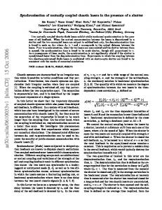
beams generated in the YAG crystal have radii 200 m. Radii are measured at 1/e2 of the maximum intensity of the Gaussian pro le. The coupling between the beams is determined by their nearest neighbor separation which can be shifted by adjusting the grating and the telescope lenses' positions. The pump beam separations and pro les are measured directly using a rotating slit method. The minimum value for nearest neighbor separation used was 0.64mm, for which there is no appreciable overlap of the pump beams and coupling is entirely due to the spatial overlap of the infrared laser elds. The couplings and detunings were chosen such that, in the absence of modulation, the lasers exhibit an instability caused by the resonance of the phase dynamics with the relaxation oscillations as described for example in [13]. The three infrared beams produced by the Nd:YAG laser are separated using a sequence of non-polarizing cube beam splitters and prisms. The intensity dynamics of the individual lasers are recorded simultaneously using fast photodiodes and a four channel digital oscilloscope. A scanning Fabry-Perot interferometer is utilized to ensure that the individual lasers have only a single longitudinal mode. Experimental measurements for the pump modulated case are displayed in Figure (2) for nearest neighbor separations of approximately 0.975 mm. Chaotic synchronization between the two outer lasers is clearly seen, whereas there is no apparent synchronization between outer and inner lasers. In the case of loss modulation they are displayed in Figure 3 for nearest neighbor separations of approximately 0.64 mm. Despite additional noise present in the loss modulated experimental set-up, chaotic synchronization between lasers 1 and 3 is readily apparent. Again, pairing intensities of lasers 1 and 2, as well as lasers 3 and 2 show little synchrony. It is interesting to note the harmonic relationships between the side lasers, 1 and 3, and the center beam, laser 2. The intensity of laser 2 oscillates at a rate approaching twice the frequency of the side beam oscillations. Fig 4 compares the power spectrums of the 4

individual beams. The dominant peak of the central beam approaches 150 KHz while the side beams display peaks at approximately 80 KHz. The sharp spike at 166 KHz is due to modulation at this frequency. The intensity time series dynamics of all three lasers was numerically estimated to be ve dimensional (Figure (5)), using a false nearest neighbors method [17], with 25000 time units considered. This result agrees with the dynamically invariant state labeled Amplitude antisynchronized in Table I, corresponding to a system with amplitude synchronization and equal left and right detunings present.

III. EQUATIONS OF MOTION The equations describing the time evolution of the slowly varying, complex electric eld amplitude Ei and real gain Gi of laser i in an array of three spatially coupled, pump modulated single mode Class B lasers are similar to those of the two laser system [15] and are as follows:

dE1 =  ?1 [(G ?  (T ))E ? E ] + i! E 1 2 1 1 dT c 1 1 dG1 =  ?1 (p (T ) ? G ? G jE j2) 1 1 1 1 f dT dE2 =  ?1 [(G ?  (T ))E ? (E + E )] + i! E 2 1 3 2 2 dT c 2 2 dG2 =  ?1 (p (T ) ? G ? G jE j2) 2 2 2 2 f dT dE3 =  ?1 [(G ?  (T ))E ? E ] + i! E 3 2 1 3 dT c 3 3 dG3 =  ?1 (p (T ) ? G ? G jE j2) 3 3 3 3 f dT

(1)

In these equations, c is the cavity round trip time, f is the uorescence time of the upper lasing level of the Nd3+ ion, and pi (T) = p0i + p1i cos( T ), i(T) = 0i + 1i cos( T ), and !i are the modulated pump parameters, modulated losses, and detunings (from a common cavity mode), respectively, of laser i. It is assumed that NOT both the pump and the 5

loss are modulated at the same time. In the Nd:YAG lasers considered in the experiments, the round trip time of light in the cavity c is 0:40 ? 0:50 ns, while the decay time of the upper lasing level f is  240s. is the modulation depth of the pump beams. is the modulation frequency and is chosen to be near the relaxation frequency. The lasers are coupled linearly to one another with strength ij , assumed to be small. For laser beams of Gaussian intensity pro le and 1=e2 beam radius w0 the coupling strength, as determined from overlap integral of the two electric elds i and j is de ned as

!

2 ij  exp ? (di 2?wd2 j ) : 0

(2)

The coupling strength is normalized such that ij = 1 if di ? dj = 0. As the coupling between lasers 1 and 3 is assumed negligible, only nearest-neighbor coupling is considered in 1. In the analysis which follows we only consider the case of loss modulation, i. e. p11 = p12 = p13 = 0, but note that the analysis is equally valid in the case of pump modulation [18]. We rst let Ei = Xiei where Xi is the amplitude and i the phase of laser i and rescale time, expressed in units of the round-trip time of light around the cavity c. We subsequently introduce L = 2 ? 1 and R = 2 ? 3 (and similarly for
L and
R ), so that we may rewrite equations 1 as the following system of ordinary dierential equations de ned on R8, i

dX1 = (F ?  (t))X ? X cos( ) 1 1 1 2 L dt dF1 = (A ? F ? F X 2 ) 1 1 1 dt dX2 = (F ?  (t))X ? (X cos( ) + X cos( )) 2 2 2 1 L 3 R dt dF2 = (A ? F ? F X 2 ) 2 2 2 dt dX3 = (F ?  (t))X ? X cos( ) 3 3 3 2 R dt 6

(3)

dF3 = (A ? F ? F X 2 ) 3 3 3 dt dL =
+ (( X2 + X1 ) sin( ) + X3 sin( )) L L R dt X1 X2 X2 dR =
+ (( X3 + X2 ) sin( ) + X1 sin( )) R R L dt X2 X3 X2 The issue of synchronization between the two outer lasers may be addressed by introducing the sum and dierence of these lasers and assuming that all three lasers are equally detuned, i. e.
L =
R = 0. Then, X13+ = 12 (X1 + X3), X13? = 21 (X1 ? X3), F13+ = 12 (F1 + F3), F13? = 21 (F1 ? F3). and synchronization between the two outer lasers occurs when X13? = F13? = 0. The transformed system is equivariant under the action of the following symmetries,

 (X+; F+; X2; F2 ; X?; F?; L ; R) = (X+; F+; X2; F2 ; ?X?; ?F?; R ; L) corresponding to interchanging the two outer lasers,

(X+; F+; X2; F2; X?; F?; L; R ) = (X+; F+; X2; F2; X?; F?; ?L ; ?R ) corresponding to conjugating the phases of the electric elds of all three lasers. There is also a parameter symmetry involving the coupling parameter  that takes (; L ; R) ! (?; L + ; R + ) which adds  onto the phase of the middle laser whilst reversing the sign of . It is interesting to note that all three lasers are phase synchronized when  is negative, corresponding to L = R = 0. However, only the two outer lasers are phase synchronized when  is positive and this is the physically relevant situation since  is assumed positive in some sense. Owing to these symmetries, the dynamically invariant subspaces illustrated in Table I exist. Notice in particular the ve dimensional subspace labeled Amplitude antisynchronized, corresponding to the case where the  symmetry has been broken, via equal detuning of 7

the two outer beams from a common cavity mode. The dimensionality of the experimental system as calculated using the false nearest neighbors method gives good agreement with this state and gives emphasis to our assumptions about the parameter regimes considered. Note that although there are several invariant subspaces where the phases of all three lasers are locked, there are NO invariant subspaces forced by symmetry such that the all amplitude and gains are equal, X+ = X2 and F+ = F2 . We may examine this using two approaches; rstly by examining the set of such points in the phase space and showing that it is not invariant (cf [19]) and secondly by reducing the system of three lasers to one of two lasers with unequal coupling. To this end, we de ne the manifold

M12 = f(X1; F1; X2; F2 ; X3; F3; L; R ) : X1 = X2 ; F1 = F2 & R = 0 or g corresponding to perfect (anti)synchronization between lasers 1 and 2 in terms of the original variables.

A. Non-invariance of M12 We demonstrate that if  6= 0, any non-zero trajectory can only be in M12 instantaneously, by assuming that X1 and X2 are non-zero and examining the evolution of the dierence x? = 21 (X1 ? X2 ) and sum x+ = 12 (X1 + X2). Note that

dx? = F1 + F2 x + F1 ? F2 x ? (t)x + x cos  + 1 X cos  : ? ? L R dt 2 ? 2 + 2 3 If the system state lies on M12 this means that x? = 0 and F1 = F2 ; so the trajectory at this point will have dx? = 1 X cos( ) R dt 2 3 Thus the trajectory must leave M12 unless  = 0, X3 = 0 and/or R = 2 + k, k 2 Z. We eliminate the rst possibility by assumption. If X3 = 0 then we note that 8

dX3 = ?X cos( ) (4) 2 R dt and so this will be non-zero as long as R 6= 2 + k for some k 2 Z, but from our de nition of M12, R = 0 or , so any trajectory satisfying (4) will not be contained in M12 . For the same reason we rule out the case R = 2 + k and this implies that a trajectory can only

be in M12 for an instant in time. As a result, M12 is ONLY an invariant subspace for the ordinary dierential equation if = 0 and the only trajectories that remain within M12 for all time have X1 = X2 = X3 = 0.

B. Reduction to a system of two lasers with unequal coupling If we assume that we lie on one of the amplitude synchronized subspaces, where X? = F? = 0, i. e. X1 = X3 and F1 = F3 , then the system (3) simpli es to a two laser system with unequal coupling between the two lasers.

dX1 = (F ? (t))X ? X cos() 1 1 2 dt dF1 = (A ? F ? F X 2) 1 1 1 dt dX2 = (F ? (t))X ? 2X cos() 2 2 1 dt dF2 = (A ? F ? F X 2) 2 2 2 dt d =  (X X ?1 + 2X X ?1) sin() 2 1 1 2 dt

(5)

Introducing sum and dierence variables in this case gives us the transformed system,

dX+ = X (F ? (t)) + F X ?  cos()(3X + X )) + + ? ? + ? dt dF+ = (A ? F (1 + X 2 + X 2 ) ? 2F X X ) + ? ? + + ? dt dX? = X (F ? (t)) + F X +  cos()(3X + X ) ? + ? + ? + dt dF? = ? (F (1 + X 2 + X 2 ) + 2F X X ) ? + ? + + ? dt 1 0 2 + 2X X + X2 ) 3( X + ? C B d =  B 32 + ?2 CA sin() @ dt (X+ ? X?) 9

(6)

If we assume that the two lasers X1 and X2 are synchronized then we nd that,

dX? =  cos()X + dt dF? = 0 dt d = 3 sin() dt

(7)

assuming that  6= 0, X+ 6= 0, then we see that X? = 0 for at most an instant in time. Since if cos() = 0 then  = 2 + k for some k 2 Z and so

d = 3 dt

(8)

which is nonzero and therefore  moves away from 2 (mod ). Consequently dXdt? moves away from 0 and so X? also moves from 0. Therefore synchronization is not achieved in the asymmetric two laser setup and thus not achieved in the original three laser system.

IV. NUMERICAL RESULTS We carried out numerical simulations independently in both the loss modulation situation as well as modulation of the pump excitation. We concentrate on the loss modulated situation due to numerical considerations, but note that our results remain valid in the case of pump modulation [18].

A. Loss Modulated Case For the loss modulated case, the simulations were performed using both Bulirsch-Stoer and Runge-Kutta integrators. Due to numerical considerations we were forced to consider more moderate values of the stiness parameter , which was of the order 0.01 and 0.001. The parameter regimes considered were also altered in order that the dierence in was taken into account. In both the cases = 0.01 and = 0.001 we saw similar results, and although the experiments were carried out with  10?6, the use of longer resonators would give a value of the stiness parameter somewhat closer to that considered numerically. We 10

carried out simulations for many values of the pump coecient and various modulation strengths for the loss. As in the model for a two laser system, in the case 0 <  1, the system undergoes a period doubling cascade to chaos as the strength of loss modulation is increased. Typically we see that for small values of the coupling parameter , there is no amplitude synchronization and the amplitude behavior of all three lasers appears to be independent, although with Antiphase synchronization between adjacent lasers. As the coupling strength is increased, a period of on-o intermittent type behavior [20], is observed in the amplitude uctuations of the two outer lasers. During this period there are times when the two outer lasers appear to be synchronized in both amplitude and phase, before bursts away from amplitude synchronization, whilst remaining completely phase (anti)synchronized. Then as the coupling strength is increased still further, there is no more bursting away from synchrony and the two outer lasers remain amplitude synchronized for all time after an initial transient phase. For the particular case where all losses are modulated equally at the rate, 0.9 + 0.2 cos ( 0.045 t ), the pump parameters were equal to 1.2 for each laser and
L =
R = 0, the behavior of a typical trajectory is as follows. Upon varying the strength of coupling , we see that there exists a critical value c  0:003125 such that for values of  < c, trajectories evolve on to the Phase Antisynchronized state. For values of  > c trajectories evolve on to the Amplitude antisynchronized state. This transition at c is strongly suggestive of a blowout bifurcation, as was the case in a system of two lasers [14]. A blowout bifurcation occurs when a normal Lyapunov exponent governing the exponential rate of change transverse to a submanifold of the total phase space passes through 0. In the case where there is more than one transverse Lyapunov exponent we need consider only the largest or normal Lyapunov exponent. If the normal exponent is negative, then on average nearby trajectories are attracted onto the submanifold and the attractor within the subspace is an attractor for the full system. If the exponent is positive then on average 11

trajectories close to the submanifold are repelled away from it. We have numerically computed the Lyapunov exponents of (3) by integrating the variational equations and examine the change that occurs in the exponents upon varying the coupling strength . These are illustrated in the case of no detunings in Fig 6. For this system, the blowout bifurcation does not occur at an isolated parameter value because the bifurcation parameter  varies the dynamics tangentially within the Antisynchronized subspace as well as those in a transverse direction from it; it is not a normal parameter for the dynamics [21,22]. Because of this (and apparent fragility of the chaotic attractors) we do not expect the Lyapunov exponents to vary smoothly or even continuously with the parameter. Hence we observe a blurred blowout [22]. The tangential variation of the dynamics is clearly indicated in gures 6 and 7, where windows of stability arise as the coupling strength  is increased. These windows of stability correspond to all Lyapunov exponents of system 3 being negative. In particular there is a window of stability shortly after the bifurcation point. In order to examine the branching behavior at blowout, we have simulated the behavior of typical trajectories that are not in any invariant subspace. Starting at c, there appears to exist a chaotic attractor A within the Antisynchronized subspace, since after an initial transient phase (which may be prolonged for some initial conditions), all trajectories eventually appear to converge to the Antisynchronized subspace. Reducing  towards c we nd regions of region of on-o intermittent type behavior, typical for a supercritical blowout. After the blowout, we no longer observe any attractors in the Antisynchronized subspace, but there is a new branch of attractors in the Phase antisynchronized subspace are created at the bifurcation. Just after c these attractors are apparently on-o intermittent and close to the antisynchronized subspace. The average position of the trajectory moves away as 12

 ! 0. This is a strong indicator that the blowout is of supercritical, soft or non-hysteretic type [16]. We also performed simulations of three loss modulated lasers in situations where the detunings were equal, i. e.
L =
R =
. We calculated the Lyapunov spectrum in this case and saw similar results to that of the purely symmetric case, with the main dierence being a bifurcation from the Amplitude antisynchronized subspace, rather than the Antisynchronized subspace. Again the blowout appears to be soft with an extended period of on-o intermittent behavior. For the particular case with parameters identical to those considered above and a value of the detuning,
= 0.001, the Lyapunov spectrum upon varying  is illustrated in gure 7. Again a blurred blowout is evident, and the normal Lyapunov exponent passes through zero at c  0:003175.

B. Pump Modulation The numerical simulations in the case of modulation of the pump excitation were carried out using a Runge-Kutta integrator with a variable timestep. Frequency of the depth of modulation was chosen so that the dynamics of the system was in a region of chaotic behavior and in this case was chosen to be 100.53 kHz (in the case of loss modulation it was 139.62 kHz). As in the case of loss modulation, excellent agreement between the experimental results and the numerical simulations are seen. A high degree of synchronization between the two outer lasers and no apparent synchronization between outer and inner laser. The transient behavior displayed similar characteristics when compared to the loss modulated simulations, such as bursts away from synchronization over short time scales, before settling on to the synchronized subspace after longer periods of time. Some of the numerical simulations we performed are illustrated in gure 8. The bi13

furcation analysis is not performed here, since the simulations indicate similar bifurcation behavior to that of the loss modulated case, as would be expected [18].

V. DISCUSSION Concluding this work, the synchronization of three Class B Nd:YAG lasers, coupled in a straight line linear array, is investigated experimentally, analytically and numerically. We investigate the separate cases of pump modulation and loss modulation both experimentally and numerically. In the experiments, a high degree of synchronization is observed between the two outer lasers of the array, whilst no synchronization is observed between outer and inner lasers. This is in good agreement with the theory, which demonstrates this lack of synchronization between outer and inner laser. In the case of loss modulation we see numerically how the loss of synchronization between the two outer lasers is lost in both the fully symmetric case and in the case with equal left and right detunings, via an apparent supercritical blowout bifurcation. This is achieved by varying the strength of coupling between the three lasers. For the experimental system, noise and symmetry breaking are both inherent, but even with quite high levels of noise, we have demonstrated a good degree of synchronization particularly in the loss modulated case. In the numerical simulations, noise and symmetry breaking have similar eects; in the region of on-o intermittency, it is unlikely that there will be a noticeable change if the perturbations are small. Low levels of noise and imperfections can result in bubbling type eects [24], which can resemble on-o intermittency in numerical simulations. Consequently, the eect of bubbling on systems such as ours is similar to the eects of on-o intermittency, namely bursts away from a synchronized state. Such bubbling persists up to a point known as a bubbling transition [25] (see also the related riddling bifurcation [26]). This situation arises when an orbit embedded in a symmetric chaotic attractor loses its transverse stability. A more detailed description of this situation may be found in [27]. 14

It is interesting to see the harmonic relationships between the central and the outer beams. Particularly for the loss modulated case with small nearest neighbor separations, the central beam appeared to be at a rate approaching twice that of the two outer beams. We conjecture that this surprising phenomenon may be caused by the central beam communicating a greater quantity of information than the two outer beams. One area of future research is to investigate these dynamics and examine the eect of parameter variation on the harmonic relationship. Although we have shown that there will be no synchronization between the outer and inner lasers in a three laser array, the question of generalized synchronization [28] arises. As we have shown, assuming that the two outer lasers are synchronized allows us to simplify the model to a system of two lasers with unequal coupling between the two lasers. This does not immediately fall into the category of generalized synchronization, since there is feedback from the "response" system into the "driving" system. However, it may still be possible to make similar conclusions to those of generalized synchronization in the case where the feedback from the one system is small compared to the input from the other. Numerical simulations of the model suggests that for small symmetry breaking perturbations of the amplitude synchronized state, an instability should arise in the phase-locking of the three lasers as predicted analytically and numerically in a system of two lasers coupled in a linear straight line array [19]. Another interesting area of future experimental work would be to heterodyne the outer beams, examine the beat frequencies over time to investigate the phase-locking instability. Such an instability may have an important bearing on maximizing power output and coherence in larger arrays of coupled lasers. JT and PA gratefully acknowledge the support of the EPSRC via grant GR/K77365. JT, KSTJ, DJD, GDV, RR and SZ gratefully acknowledge support from the Oce of Naval Research. It is a pleasure to also thank the nancial support from Georgia Institute of Technology and China Scholarship Council (S.Z.). Finally we should like to thank Steve Strogatz 15

and Henry Abarbanel for a helpful discussion concerning generalized synchronization.

16

REFERENCES [1] L. M. Pecora and T. L. Carroll, Phys. Rev. Lett. 64, 821 (1990). [2] L. M. Pecora and T. L. Carroll, Phys. Rev. A 44, 2374 (1991). [3] K. M. Cuomo and A. V. Oppenheim, Phys. Rev. Lett. 71, 65 (1993). [4] L. Kocarev and U. Parilz, Phys. Rev. Lett. 74, 5028 (1995). [5] G. D. VanWiggeren and R. Roy, Science, 279, 1198 (1998). [6] G. D. VanWiggeren and R. Roy, Chaotic Communication Using Time-Delayed Optical Systems, Preprint, submitted to Int. J. Bif. Chaos [7] A. V. Gaponov-Grekhov, M. I. Rabinovich and I. M. Starobinets, Pis'ma v Zh. Eksp. Teor. Fiz. 39, 561 (1984). [8] V. S. Afraimovich, N. N. Verichev and M. I. Rabinovich, Izvest. Vyss. Uch. Zavedenii, Radio zika 29, 1050 (1986). [9] S. K. Han, C. Kurrer and Y. Kuramoto, Phys. Rev. Lett. 75, 3190 (1995). [10] H. G. Winful and L. Rahman, Phys Rev. Lett. 65, 1575 (1990). [11] L. Fabiny, P. Colet, R. Roy, D. Lenstra, Phys. Rev. A 47, 4287 (1993). [12] R. Roy and K. S. Thornburg, Jr., Phys. Rev. Lett 75, 3190 (1995). [13] K. S. Thornburg, Jr., M. Moller, R. Roy, T. W. Carr, R.-D. Li, T. Erneux, Phys. Rev. E 55, 3865 (1997). [14] P. Ashwin, J. R. Terry, K. S. Thornburg, Jr. and R. Roy, To appear Phys. Rev. E. 1998 [15] R. Roy and K. S. Thornburg, Jr., Phys. Rev. Lett. 72, 2009 (1994). [16] E. Ott and J. C. Sommerer, Phys. Lett. A 188, 39 (1994). [17] H. D. I. Abarbanel, Analysis of Observed Chaotic Data, Springer (1996). 17

[18] J. R. Tredicce, N. B. Abraham, G. P. Puccioni, and F. T. Arecchi, Opt. Commun. 55, 131 (1985). [19] J. R. Terry, Detuning and Symmetry breaking in a system of coupled chaotic lasers. Preprint. [20] N. Platt, E. A. Spiegel and C. Tresser, Phys. Rev. Lett. 70 (1993) 279 [21] P. Ashwin, J. Buescu, and I. N. Stewart, Nonlinearity 9, 703 (1996). [22] P. Ashwin, E. Covas, and R. Tavakol, Technical Report No. 98/3, Dept of Maths and Stats, University of Surrey (1998). [23] P. Colet and R. Roy, Opt. Lett. 19, 2056 (1994). [24] P. Ashwin, J. Buescu, and I. Stewart, Phys. Lett. A 193, 126 (1994). [25] S. C. Venkataramani, B. R. Hunt, E. Ott, D. J. Gauthier and J. C. Bienfang, Phys. Rev. Lett. 77, 5361 (1996). [26] Yu. L. Maistrenko, V. L. Maistrenko, A. Popovich and E. Mosekilde, Phys. Rev. E. 57, 2713 (1998). [27] Y.-C. Lai, C. Grebogi, J. A. Yorke and S. C. Venkataramani, Phys. Rev. Lett. 77, 55 (1996). [28] N. F. Rulkov, M. M. Sushchik, L. S. Tsimring and H. D. I. Abarbanel, Phys. Rev. E. 51, 980 (1995).

18

TABLES Symmetry Z2 ()  Z2 ()00 Z2()  Z2() Z2() Z2()00 Z2()

Representative point (X+ ; F+ ; X2 ; F2 ; 0; 0; 0; 0) (X+ ; F+ ; X2 ; F2 ; 0; 0; ; ) (X+ ; F+ ; X2 ; F2 ; 0; 0; ; ?) (X+ ; F+ ; X2 ; F2 ; X? ; F? ; 0; 0) (X+ ; F+ ; X2 ; F2 ; X? ; F? ; ; )

Dim. 4 4 5 6 6

Name Synchronized Antisynchronized Amplitude antisynchronized Phase synchronized Phase antisynchronized

TABLE I. Dynamically invariant subspaces in Eqs. 3. A list of symmetry forced invariant subspaces of the equations for a system of three linearly coupled lasers. We have listed only those states which contained an attractor in the numerical simulations. Note that other states exist but are not seen as attracting for the system.

19

FIGURES

AOM b

AOM

a

FIG. 1. Experimental system for generating three laterally coupled lasers in a Nd:YAG crystal and observing the synchronization of chaotic laser intensities. A diractive optic is used to split the Argon laser into three beams with almost equal intensities. The three beams are made parallel by a telescope; changing the magni cation of the telescope changes the separation d between each laser. An Acousto-Optic Modulator (AOM) is placed in position (a) in the case of loss modulation and in position (b), in the case of pump modulation. The Nd:YAG crystal is coated for high re ectivity (HR) on one side and antire ection coated (AR) on the other. The output coupler (OC) is 2% transmissive; both mirrors are at. A CCD camera is used to measure the far- eld intensity pattern of the array, while the three photodetectors PD1, PD2, and PD3 simultaneously measure each lasers' intensity dynamics, which are subsequently recorded on a digital sampling oscilloscope (DSO).

20

Intensity of Laser 2

Intensity of Laser 1

40 30 20 10 0

0

500

1000

1500

2000

50 40 30 20 10

0

10

20

30

50

Intensity of Laser 3

Intensity of Laser 2

Intensity of Laser 1

40 30 20 10

0

500

1000

1500

2000

40 30 20 10 0

0

10

20

30

40

Intensity of Laser 2

Intensity of Laser 3

Intensity of Laser 1

30 20 10 0

0

500

1000 Time (µs)

1500

2000

50 40 30 20 10

0

10

20

30

Intensity of Laser 3

FIG. 2. Experimental measurements of the relative intensities of three coupled lasers for pump beam separations d = 0.975 mm and modulation depth p1i = 0.20 (for i=1,2,3). A high degree of intensity synchronization is seen only between lasers 1 and 3.

21

Laser 1 Intensity Time Series

Laser 1 Intensity vs Laser 2 Intensity

250

200 180

Laser 2 Intensity

Laser 1 Intensity

200 150 100 50 0 1200

160 140 120 100 80

1400

1600 Time (µs)

60

1800

0

Laser 2 Intensity Time Series

50

100 150 Laser 1 Intensity

200

250

Laser 1 Intensity vs Laser 3 Intensity

200

200

160

Laser 3 Intensity

Laser 2 Intensity

180

140 120 100

150

100

50

80 60 1200

1400

1600 Time (µs)

0

1800

0

Laser 3 Intensity Time Series

50

100 150 Laser 1 Intensity

200

250

Laser 3 Intensity vs Laser 2 Intensity

200

200

150

Laser 2 Intensity

Laser 3 Intensity

180

100

50

160 140 120 100 80

0 1200

1400

1600 Time (µs)

60

1800

0

50

100 150 Laser 3 Intensity

200

FIG. 3. Experimental measurements of the relative intensities of three coupled lasers with loss modulation. Here the nearest neighbor separation d = 0.64 mm. Once again, a high degree of intensity synchronization is seen only between lasers 1 and 3.

22

Power Spectrum of Beam 1

6

Power (arbitrary units)

10

4

10

2

10

0

10

50

100

150

200 250 300 Frequency (KHz)

350

400

450

500

350

400

450

500

350

400

450

500

Power Spectrum of Beam 2

6

Power (arbitrary units)

10

4

10

2

10

0

10

50

100

150

200 250 300 Frequency (KHz) Power Spectrum of Beam 3

6

Power (arbitrary units)

10

4

10

2

10

0

10

50

100

150

200 250 300 Frequency (KHz)

FIG. 4. Power spectrum of three linearly coupled lasers, in the case of loss modulation at a rate of 166KHz. Here the nearest neighbor separations are again 0.64mm. Notice the peak in the central beam close to 150KHz which is not present in the two outer beams. However, the side beams display a peak at approximately 80KHz of a greater intensity than the corresponding peak in the central beam . The peak in all beams at 166KHz corresponds to modulation at this rate.

23

Dimension of Loss Modulated Intensity Time Series

Percentage of False Nearest Neighbors

100

80 Laser 1 Laser 2 Laser 3

60

40

20

0 0

2

4

6

8

10

Dimension

FIG. 5. Using the false nearest neighbors method, we numerically estimate the dimensionality of the experimental system, using measured time series of the intensity uctuations. The 1% mark suggests that the system is ve dimensional, giving good agreement between the experiments and the dimensionality of the model.

24

0.015

0.005

λ_ ι

Λ1 λ1

−0.005

−0.015

−0.025 0.001

0.002

0.003

κ

0.004

0.005

FIG. 6. Lyapunov exponent diagram in the case of modulated loss. The parameter values for the lasers were assumed identical and were 0i = 0.9, 1i = 0.2, pi = 1.2 (for i=1,2,3). We assumed the detunings of the lasers were such that
L =
R = 0. We have labelled the largest tangential Lyapunov exponent 1 . Notice that this is positive for most values of the coupling strength . The non-normality of  is apparent through the windows of stability that arise when varying . These correspond to the periods where 1 is negative. The blowout occurs when the normal Lyapunov exponent, 1 passes through 0. In this case this occurs for   0.003125

25

0.015

0.005

Λ1 λ1

λ_ι

−0.005

−0.015

−0.025

−0.035 0.001

0.003

κ

0.005

0.007

FIG. 7. Lyapunov exponent diagram in the case of modulated loss. Here the detunings were assumed equal with
L =
R = 0.001 and the exponents were plotted upon varying the strength of coupling . The parameter values for the lasers were assumed identical and were once again 0i = 0.9, 1i = 0.2, pi = 1.2 (for i=1,2,3). We have labelled the largest tangential Lyapunov exponent 1 and the normal Lyapunov exponent 1 . Similar behavior to the case of no left and right detuning is seen. However, the point of blowout is altered, in this case   0.003175

26

8 Intensity of Laser 2

Intensity of Laser 1

4

2

0 1000

2000

6 4 2 0

3000

0

2

4

Intensity of Laser 1

4 Intensity of Laser 3

Intensity of Laser 2

8 6 4 2 0 1000

2000

2

0

3000

0

2

4

Intensity of Laser 1

8 Intensity of Laser 2

Intensity of Laser 3

4

2

0 1000

2000

3000

Time (µs)

6 4 2 0

0

2

4

Intensity of Laser 3

FIG. 8. Numerical simulated three laser model with pump modulation. The modulation rate was again chosen to be near the relxation oscillation frequency of the lasers so as to induce chaotic

uctuations in the intensities.

27