Progress in Computational Fluid Dynamics, Vol. x, No. x, 200x
1
Synthetic turbulent inflow conditions based on a vortex method for large-eddy simulation Sofiane Benhamadouche* EDF R&D Dept. MFTT, 06 Quai Watier, 78401 Chatou Cedex, France E-mail:
[email protected] *Corresponding author
Nicolas Jarrin and Yacine Addad UMIST, MAME Dept. Thermo-Fluids div., Manchster M60 1QD, UK E-mail:
[email protected] E-mail:
[email protected]
Dominique Laurence EDF R&D Dept. MFTT, 06 Quai Watier, 78401 Chatou Cedex, France E-mail:
[email protected] Abstract: The generation of ‘synthetic turbulence’ for inflow conditions in Large Eddy Simulation is investigated. The method is based on a 2D vortex method for the lateral components of the fluctuating velocity and a 1D Langevin equation for the streamwise velocity component, mimicking a Restress transport model. Channel flow at Reτ = 395 and pipe flow at Reτ = 360 are used to test the ‘synthetic turbulence’ alone in the 2D inlet plane, then LES computations are run with these inlet conditions. Finally, the method is applied to a backward facing step with and without heat transfer. Keywords: large-eddy simulation; synthetic turbulence; inflow boundary conditions; channel; pipe and back-step flow. Reference to this paper should be made as follows: Benhamadouche, S., Jarrin, N., Addad, Y. and Laurence, D. (xxxx) ‘Synthetic turbulent inflow conditions based on a vortex method for large-eddy simulation’, Progress in Computational Fluid Dynamics, Vol. x, No. x, pp.xxx–xxx. Biographical notes: S. Benhamadouche graduated from ENPC Paris in 2000, obtained his DEA in numerical analysis in 2000 and Mphil in 2001 at UMIST and continued with a PhD on unstructured finite volumes for LES, while also developing the code_Saturne CFD software at EDF R&D, and lecturing at ENPC. N. Jarrin graduated in 2003 from Ecole Nationale des Ponts et Chaussées, Paris (ENPC), then obtained his MSc at U. of Manchester (UMIST) in 2004, where he is continuing research on synthetic turbulence generation through a PhD. Y. Addad graduated from U. Oran, obtained his MSc at UMIST in 2000, then a PhD in 2005 on LES with unstructured grids. D. Laurence is a Professor of CFD at U. of Manchester (UMIST) since 1999 and research engineer at EDF R&D where he has also developed CFD software and turbulence models since 1980. Prior Manchester, he lectured fluid mechanics at ENPC for 15 years.
1
Introduction
Large Eddy Simulation (L.E.S.) is becoming widely used in some industrial applications (Mahesh et al., 2001; Benhamadouche et al., 2003; Benhamadouche and Laurence, 2003). In many cases as with bluff body
Copyright © 200x Inderscience Enterprises Ltd.
separation, free shear layers and periodic obstacles, the problem of inlet conditions is reduced by the presence of a strong turbulence generation process inside the domain. To tackle a wider range of industrial cases via L.E.S., there is a need to develop unsteady inflow conditions with more realistic physical properties.
2
S. Benhamadouche, N. Jarrin, Y. Addad and D. Laurence
During the last decade, several attempts to create inlet fluctuations have been made (Balaras et al., 2000; Kondo et al., 1997; Lund, 1998). The most widely used accurate method consists in conducting a preliminary computation of turbulent flow field, using L.E.S., such as boundary layer flows (Koutmos and Mavridis, 1997), then to use the results of this computation as inlet conditions. This precursor simulation method is successful; however it entails a large computational load (both for data storage and CPU time). The other popular approach uses a mean velocity profile and a level of turbulent kinetic energy (or a profile when available). With these two data, random noise perturbations (based for example on a gaussian distribution) are added to the velocity components to obtain the desired statistical quantities (mean velocity and turbulent energy). This approach was adopted by Addad et al. (2002) in a L.E.S. of a forward–backward facing step and Benhamadouche et al. (2003) in an L.E.S. with heat transfer in a T-junction. The results in both cases were satisfactory. The method, however, is known to be less suited for cases where inflow conditions play a major role in the development of boundary layers. Recently, Sergent (2002) developed a new method to generate fluctuations that, unlike the random noise, contains some spatial correlations. The approach is based on generating random vortices in the inlet flow plane (normal to the streamwise velocity) for the wall-normal components, which gives a spatial correlation, and on the generation of the streamwise component using a Langevin equation, which provides a temporal correlation, as well as with the two cross-stream components. In the present work, this method has been further developed and adapted to the in-house EDF code Code_Saturne (Archambeau et al., 2004). The method is also extended to pipe flows with some minor modifications. After some 2D and 3D tests with channel and pipe flows, the vortex method is used on a backstep flow with and without heat transfer and compared to the more widely used methods: precursor channel flow and a random noise method (Lund, 1998).
2
Numerical methods
2.1 Vortex method A short description of the vortex method is given in this section; more details can be found in Sergent (2002). U = (u, v, w) is the velocity vector, u, v and w are respectively the streamwise, the wall normal and the spanwise components. The method is based on a Lagrangian approach of Navier-Stokes equations. The centres of the vortices are transported and the vorticity is given a certain distribution. In the following, V = (v, w) , ω is the vorticity (the rotational of V ) and x is a 2D position vector. The vorticity generated by the vortex i at a point x is given by
ωi ( x) = Γiξσ ( x − xi ) i
where xi is the centre of the vortex, σi its diameter (in the following a characteristic length of the support of the shape function), Γi its intensity and ξσ i a shape function. Only an improved gaussian form found in Sergent (2002) is tested in this paper. x x 1 1 − 2σ i2 − 2σ i2 . − 2 1 ξσ i ( x) = e e 2π σ i 2 2
2
If n is the number of vortices, the vorticity is: n
ω ( x) = ∑ Γiξσ ( x − xi ). i
i =1
Then, the components (v,w) are obtained by using a Biot and Savart kernel V ( x) = −
1 2π
n
∑ Γ K σ ( x) i =1
i
i
with, x
2
x
2
⊥ − − x− y −1 2σ i 2 2σ i 2 x K σ i ( x) = ξ y y e e ( )d (1 ) . ∧ = − σi 2 2π ∫∫ x − y 2 x
One needs to specify the parameters that have been previously introduced. The most important parameter is certainly the circulation Γi, because it is through this parameter that one will be able to control the intensity of the fluctuations. One can find in Sergent (2002), a formula giving Γi as a function of the vorticity or the turbulent kinetic energy. As turbulent kinetic energy is more likely to be available (for example from a R.A.N.S. calculation), one focuses on this method. The formula is obtained by calculating the rms fluctuations of the velocity (by integrating the velocity formula over the inlet plane, assuming that the plane is finite) and by identifying it with a given profile of turbulent kinetic energy. The circulation is estimated by: Γi ≈ 4
π Sk ( xi )
3n [ 2 ln(3) − 3ln(2) ]
where S is the 2D inlet surface and k the turbulent kinetic energy. At the first time step, the vortex positions are given randomly in the 2D plane. The vortices are then given a random rotation sense. A characteristic time (the turbulent time scale τ = k/ε) is defined for each vortex. If the lifetime of the vortex exceeds this characteristic time, then the vortex is destroyed and a new one is generated randomly in the inlet plane. Note that the initial time for each vortex is determined randomly. The diameter σi of the vortices has also to be set. One can use a turbulent length scale approach (l = k3/2/ε) or a constant value. In the simulations surveyed,
Synthetic turbulent inflow conditions based on a vortex method for large-eddy simulation it is taken constant. Other tests will be made in the future by introducing the Taylor scale and some limiters based on the Kolmogorov scale. Then, the vortices are attributed a random walk in the inflow plane to develop fluctuations in time. Finally, appropriate vortex method techniques in 2D are used to specify boundary conditions (periodic boundary conditions, solid-wall and symmetry conditions). This consists in introducing ghost vortices so that the velocity at the wall, which is the sum of the velocity because of the real vortices and the ghost vortices, is zero. The way the ghost vortices are generated is explained in Sergent (2002). An improvement for the wall conditions is introduced in the present work, so that the method can cope with all shapes of walls. The method is explained in Figure 1. For each point M where the velocity has to be computed, one takes its orthogonal projection on the wall (point P on the Figure). Then for each vortex, a ghost vortex is generated taking its symmetric related to the point P. For periodic boundary conditions, the domain is shared in two parts and ghost vortices are generated with respect to the periodicity. Thus, the velocity field is the same at the corresponding periodic boundaries. Figure 1
Generation of ghost vortices, wall conditions (left), periodic conditions (right)
2.2 Langevin equation for the streamwise component To generate the streamwise fluctuations, Langevin equation is used, which is slightly different from the one introduced by Sergent (2002). The simplest Langevin equation for a random variable ui′ is: dui ' = −
ui′ dt + (c0ε )0.5 dWi (t ) T
where Wi is a Wiener process and T, c0 and ε are the constants. One estimates dui′u ′j / dt and identifies the different terms with the help of the Reynolds Stress Equations of the LRR model (Launder et al., 1975). One then obtains the values of T, c0 and ε. The method used by Sergent (2002) was based on the assumption that the three velocity fluctuations were satisfying a Langevin equation. In our approach, it is preferred to neglect some terms then to suppose that 1 c du ' dW (t ) 2 ∂u = − 1 u '+ c2 − 1 v '+ (c0ε ) 2 dt 2T dt 3 ∂y
with T=
k
ε
, c0 =
14 , c1 = 1.8 and c2 = 0.6. 15
3
2.3 Numerical procedure for L.E.S The flow is assumed incompressible and Newtonian, and the density is only function of the temperature. The turbulent viscosity µt is given by the standard Smagorinsky model:
µt = (Cs ∆) 2 2 Sij Sij where Sij is the filtered strain-rate tensor and ∆ the length scale of the filter. In the framework of a finite volume approach using hexahedral cells, one may consider ∆ = 2Ω1/3, where Ω is the volume of the cell. The Smagorinsky constant Cs is set to 0.065 (this is a common value for channel flow simulation at moderate Reynolds numbers) or computed dynamically by using a dynamic model based on Germano’s identity. Regarding near-wall modelling, a power law wall function is used and the turbulent viscosity is damped with a Van Driest damping function. More details on L.E.S. in Code_Saturne can be found in Benhamadouche and Laurence (2003) and Benhamadouche et al. (2002). In the collocated finite volume approach used in Code_Saturne, all variables are located at the centres of gravity of the cells. The momentum equations are solved uncoupled by considering an explicit mass flux. Velocity and pressure coupling is insured by a prediction/ correction method with a SIMPLEC algorithm (Ferziger and Perić, 1999). The Poisson equation is solved with a conjugate gradient method with a diagonal preconditioning. The collocated discretisation requires a Rhie and Chow (1983) interpolation in the correction step to avoid oscillatory solutions with Cartesian meshes. For L.E.S. calculations, second order schemes are used in space (fully centred scheme for the velocity components, centred scheme with a slope test for the temperature) and time (Crank-Nicolson with a linearised convection). A second order Adams-Bashforth time advancing scheme is used for the mass flow and the part of the diffusion involving the transposed velocity gradient, to keep the velocity components uncoupled. A reconstruction technique is also used to compute the gradients at the non-orthogonal faces (Archambeau et al., 2004).
3
2D inlet plane tests
3.1 Channel flow Reτ = 395 This section is related to the validation of the vortex method approach as implemented in Code_Saturne for the 2D inlet plane in a fully developed channel flow. This configuration was already treated by Sergent (2002). The 2D domain is a 2δ × 2δ square. Analytical functions deduced from the channel flow statistics are used to scale the inlet fluctuations. As the mean profile is imposed for u, the plots are only given for rms quantities. Sergent (2002) studied the sensitivity of the method to different parameters. It was found to be stable towards time iteration and converges as the number of vortices increases.
4
S. Benhamadouche, N. Jarrin, Y. Addad and D. Laurence
The size of the vortices (parameter σi) appeared to have a non-negligible influence on the position of the peak of the fluctuations; the bigger the vortices, the further away from the wall the peak is. For the next calculation, reasonable values of σi and n are imposed (σi = 0.1 and n = 100). Figure 2 shows the coherent structures in the wall region, the tangential velocity field looks like a turbulent one. Figure 3 shows 2nd order rms profiles compared to DNS data from Kim et al. (1987). The same conclusion as in Sergent (2002) can be drawn from these results. The rms fluctuations of the velocity components are well represented, and energy levels at the centre of the channel are in good agreement with the experiment. One can notice that the profiles of v′ and w′ are similar to the 2/3k profile of the DNS. This is because of the fact that the circulation of our vortices is based on the k profile. One way to improve these profiles is to use, if available (if one uses a Reynolds Stress Model), v′ and w′ profiles to compute the recirculation. This has been recently tested and gives satisfactory results. The correlation u ′v′ (representative of the shear stress) is also represented. Its shape comes actually from the shape of ∂u / ∂y , which is imposed in the Langevin equation. It may be improved by incorporating turbulent transport processes in the Langevin equation (transporting the structures by themselves). Figure 2
as pipes are more encountered in industrial cases. As a reference, one uses the D.N.S. simulations of Eggels et al. (1993). Figure 4 shows the ‘synthetic’ structures that, although generated in a second, have an L.E.S. ‘look’. One can notice the efficiency of our boundary conditions where the velocity vanishes perfectly. In Figure 5, the rms values v ′2 and w′2 are again well qualitatively reproduced. One can notice the same behaviour as for the channel flow case. The u ′v ′ profile’s shape comes from the shape of ∂u / ∂y , which is imposed in the Langevin equation. The shape of v ' and w′ profiles comes from the profile of 2/3k on which the circulation is based. Figure 3
rms profiles (2D channel flow)
Figure 4
Velocity field (vortex method, pipe flow)
Velocity field (vortex method, channel flow)
3.2 Pipe Flow Reτ = 360 The method has been extended to pipe flows with the appropriate modifications for wall boundary conditions,
Synthetic turbulent inflow conditions based on a vortex method for large-eddy simulation Figure 5
4
rms profiles (2D pipe flow)
L.E.S. tests
4.1 Channel flow Reτ=395 A proper channel flow L.E.S. with Reτ = 395 is now computed (statistics shown now correspond to the L.E.S.) using the inlet conditions generated by the vortex/Langevin method. The computational domain is 30δ × 2δ × πδ, so that the length of the domain is sufficient to study the development of the fluctuations generated by our method at the inlet. The number of nodes is 149 × 68 × 25. The maximum Courant number during the simulation is 2. As can be seen in Figures 6 and 7, rms profiles have an appropriate behaviour from around x/δ = 12 onwards. Figure 6
rms profiles at different streamwise positions for the 3D channel flow at Reτ = 395
Figure 7
rms profiles ( u′2 and u′v′ ) for the 3D channel flow at Reτ = 395
The turbulence generated by the vortex/Langevin method is acceptable still closer to the inlet (after x = 2δ it starts to redevelop). Sergent (2002) chose to counter the initial decay by introducing a control plane to calibrate the inlet kinetic energy, amplifying the level at the inlet to recover the desired level in the control plane. This type of solution cannot be easily implemented in an industrial context. Moreover, the low levels of v ′2 and w′2 are a common feature of L.E.S. calculations, where a large part of the turbulence spectrum lies in the subgrid-scales. The D.N.S. results are approached only when the mesh is significantly refined.
4.2 Pipe flow Reτ = 360 The pipe flow is tested with Reτ = 360 D.N.S. simulations of Eggels et al. (1993). The length of computational domain is 30R in the streamwise direction, where R is the pipe radius so that the length of the domain is sufficient to study the development of the fluctuations generated by our method at the inlet. The number of cells is around 290,000. The maximum Courant number during the simulation is 2. Figure 8 shows rms profiles at different locations. One can observe that the results are quite satisfactory. The turbulence develops rapidly from the inlet plane and has very realistic rms profiles from x = 10R. Like in the channel flow test case, the fluctuations are really acceptable close to the inlet plane. This is a promising result for industrial cases, which often use inlet boundary conditions for pipes. Figure 8
On the other hand, purely random fluctuations imposed at inlet or Langevin equation imposed on the three velocity components decayed rapidly, and the turbulence did not even recover before the end of the computational domain.
5
rms profiles at different streamwise positions for the 3D pipe flow at Reτ = 360
6
S. Benhamadouche, N. Jarrin, Y. Addad and D. Laurence
4.3 Backstep flow Re=5100 The reference case is taken from Le and Moin (1992). The case is isothermal and the Reynolds number, based on the step height h and the mean inlet free stream velocity, is Reh = 5100. The height of the upstream section is 5h. The mesh contains 150,000 cells. The standard Smagorinsky subgrid scale model is used with a constant equal to 0.065. The statistics are now integrated over time and in the homogeneous direction of the flow (the spanwise direction). In addition to the vortex/Langevin method, a computation with a precursor L.E.S. channel flow and one with the Random Fluctuation Inflow Generation Method (RFIGM) found in Lund (1998) are performed. One can observe in Figures 9–11 (only the random calculation is represented to make the figure clearer) that the mean and rms quantity u′v′ step are well predicted with the vortex method. It gives almost the same results as the one that uses the precursor calculation. The random fluctuations give an over-estimation of the recirculation region (the purely random fluctuations without any coherence in time as in the present method give a much delayed reattachment). Figure 12 gives the predicted friction coefficient compared to DNS data. One can see that both LES, with the vortex method or the precursor channel calculation, gives satisfactory results. Table 1 summarises the predicted recirculation lengths and confirms our statement. Figure 9
Figure 11 u′v′ profile at four downstream positions (backstep flow, Reh = 5 100)
Figure 12 Friction coefficient profile (backstep flow, Reh = 5 100)
u profile at four downstream positions (backstep flow, Reh = 5 100)
Table 1
Recirc. length (x h)
Recirculation length D.N.S.
Preliminary L.E.S.
Random
Vortex
6.18
5.76
7.47
6.65
4.4 Backstep flow with heat transfer
Figure 10 v profile at four downstream positions (backstep flow, Reh = 5 100)
The case is taken from Avancha and Pletcher (2002). The step and the upstream section heights are respectively h and 2h. The Reynolds number based on h and the upstream centreline velocity is 5540. The bottom wall downstream of the step is applied with a uniform wall heat flux (1 kW/m²). The Prandtl number is equal to 0.71. The molecular viscosity and the conductivity are variable and given by a power-law: µ / µ 0 = (T / T0 ) Pr, λ / λ0 = (T / T0 ) Pr . The mesh contains only 150,000 cells. The dynamic model based on Germano’s identity has been used, in which the dynamic Smagorinsky constant is averaged in time and space (in the homogeneous direction). Figure 13 shows the streamlines obtained with the mean average velocity vector. The recirculation zone is well captured with a recirculation length equal to 6.26h (the isothermal experiment of Kasagi and Matsunaga (1995) gives 6.51h, and Avancha and Pletcher (2002) calculation gives 6.1h). The secondary
Synthetic turbulent inflow conditions based on a vortex method for large-eddy simulation recirculation is also visible. The Wall temperature is plotted in Figure 14. The same behaviour, as the one observed by Avancha and Pletcher (2002) is obtained. A peak is observed around x/h = 1 reaching 480 K. The flow is stagnant in this region, and heat transfer is mainly because of conduction phenomena. Away from this region, the temperature decreases owing to convection. Further downstream, a linear increase of the temperature is observed. This is because of the development of a thermal boundary layer after the reattachment zone. Figure 13 Mean-flow streamlines (backstep flow Re = 5 540)
Figure 14 Wall temperature downstream the step (backstep flow, Re = 5 540)
5
Conclusions
The vortex/Langevin method has been implemented in EDF in-house industrial code, Code_Saturne. After some improvements of the method concerning the treatment of boundary conditions and some physical parameters (the diameter of the vortices and their life-time), the method has been extended to cylindrical geometries and gave very satisfactory results either in 2D or in 3D for the pipe flow. With the vortex method, the flow becomes fully developed after a certain length and gives satisfactory levels of turbulence, whereas this is not the case with any random generation method. Moreover, two back step flows, with and without heat transfer, have been tested. The results are again far better than with a random method and comparable to those obtained with the precursor channel flow L.E.S. method. The method is expected to be of much industrial interest, avoiding costly precursor simulations and data storage. Moreover, these results are encouraging for future
7
R.A.N.S./L.E.S. coupling, i.e., that would enable a local L.E.S. embedded in a global R.A.N.S industrial simulation.
References Addad, Y., Laurence, D., Talotte, C. and Jacob, M.C. (2002) ‘Large eddy simulation of a forward-backward facing step for acoustic source identification’, 5th Int. Symposium on Engineering Turbulence Modelling and Experiments, Elsevier. Archambeau, F. Méchitoua, N. and Sakiz, M. (2004) ‘Code_saturne: a finite volume code for the computation of turbulent incompressible flows – industrial applications’, Int. J. on Finite Volumes, Web based journal, only available electronically, Febrary 2004. Avancha, R.V.R. and Pletcher, R.H. (2002) ‘Large eddy simulation of the turbulent flow past a backward-facing step with heat transfer and property variations’, Int. Journal of Heat and Fluid Flow, Vol. 23, pp.601–614. Balaras, N., Li. E. and Piomelli, U. (2000) ‘Inflow conditions for Large-eddy simulations of mixing layers’, Phys. Of Fluids, Vol. 12, No. 4, pp.935–938. Benhamadouche, S. and Laurence, D. (2003) ‘LES, coarse LES, and transient RANS comparisons on the flow across tube bundle’, Int. J. Heat and Fluid Flow, Vol. 4, pp.470–479. Benhamadouche, S., Mahesh, K. and Constantinescu, G. (2002) ‘Collocated finite volume schemes for L.E.S. on unstructured meshes’, CTR, Proceeding of the 2002 Summer Program Stanford University, NASA and CTR, pp.143–154. Benhamadouche, S., Sakiz, M., Péniguel, C. and Stéphan, J.M. (2003) ‘Presentation of new methodology of chained computations using instationary 3D approaches for the determination of thermal fatigue in a T-junction of a PWR nuclear plant’, 17th International Conference on Structural Mechanics in Reactor Technology (SmiRT17), August, Prague, pp.17–22. Eggels, J.G.M., Unger, F., Weiss, M.H., Westerweel, J., Adrian, R.J., Friedrich, R. and Nieuwstadt, F.T.M. (1993) ‘Fully developed turbulent pipe flow: a comparison between direct numerical simulation and experiment’, J. Fluid Mech., (1994), Vol. 268, pp.175–209. Ferziger, J.H. and Períc, M. (1999) Computational Methods for Fluid Dynamics, 2nd ed., Springer. Kasagi, N. and Matsunaga, A. (1995) ‘Three-dimensional particle-tracking Velocimetry measurement of turbulence statistics and energy budget in a backward facing step flow’, Int. J. Heat Fluid Flow, Vol. 16, No. 6, pp.477–485. Kim, J., Moin, J.K.P. and Moser R. (1987) ‘Turbulence statistics in fully developed channel flow at low Reynolds number’, J. Fluid Mech., Vol. 177, pp.133–166. Kondo, K.S., Murakami, S. and Mochida, A. (1997) ‘Generation of velocity fluctuations for inflow boundary condition for LES’, J. Wind Eng. and Ind. Aero., Vols. 67–68, pp.51–64. Koutmos, P. and Mavridis, C. (1997) ‘A computational investigation of unsteady separated flows’, Int. J. Heat and Fluid Flow, Vol. 18, pp.297–306. Launder, B.E., Reece, G.J. and Rodi, W. (1975) ‘Progress in the development of a Reynolds-stress turbulence closure’, Journal of Fluid Mechanics, Vol. 68, pp.537–566. Le, H. and Moin, P. (1992) ‘Direct numerical simulation of turbulent flow over a backward-facing step’, Stanford Univ., Center for Turbulence Research, Annual Research Briefs, pp.161–173.
8
S. Benhamadouche, N. Jarrin, Y. Addad and D. Laurence
Lund, T.S. (1998) ‘Generation of turbulent inflow data for spatially-developing boundary layer simulations’, Journal of Computational Physics, Vol. 140, pp.233–258. Mahesh, K., Constantinescu, G., Apte, S., Iaccarino, G. and Moin, P. (2001) ‘Large eddy simulation of gas turbine combustors’, Annual Research Briefs, Center for Turbulence Research, NASA Ames/Stanford Univ., pp.3–19.
Rhie, C.M. and Chow W.L. (1983) ‘A numerical study of a turbulent flow past an isolated airfoil with trailing edge separation’, AIAA Journal, Vol. 21, No. 11, pp.1525–1532. Sergent, M.E. (2002) Vers une Méthodologie de Couplage Entre la Simulation des Grandes Echelles et les Modèles Statistiques, Phd Thesis, Ecole Central de Lyon.