and Physics
cess
Atmospheric Measurement Techniques
Open Access
Biogeosciences
Open Access
Atmos. Meas. Tech., 6, 2169–2179, 2013 www.atmos-meas-tech.net/6/2169/2013/ doi:10.5194/amt-6-2169-2013 © Author(s) 2013. CC Attribution 3.0 License.
of the Past
J. Danzer1,2 , B. Scherllin-Pirscher1,2 , and U. Foelsche1,2 1 Wegener
Center for Climate and Global Change (WEGC), University of Graz, Graz, Austria for Geophysics, Astrophysics, and Meteorology/Institute of Physics (IGAM/IP), University of Graz, Graz, Austria
Earth System Dynamics
Correspondence to: J. Danzer (
[email protected])
Received: 14 December 2012 – Published in Atmos. Meas. Tech. Discuss.: 20 February 2013 Revised: 22 July 2013 – Accepted: 23 July 2013 – Published: 29 August 2013
Open Access
Geoscientific
bending angle data, by using the bending angle bias characInstrumentation teristics of a solar cycle as a correction factor. After the cliMethods and matological ionospheric correction the bias of the simulated Data Systems data improved significantly, not only in the bending angle but also in the retrieved temperature profiles.
1
Geoscientific Model Development Introduction and motivation
Open Access
The radio occultation (RO) method (Melbourne et al., 1994; Kursinski et al., 1997; Hajj et al., 2002) is an active satelHydrology and lite to satellite limb sounding technique. Measurements are System performed when a globalEarth positioning system (GPS) satellite transmits an electromagnetic signal, which is recorded Sciences at a low earth orbit (LEO) satellite. The path of the transmitted electromagnetic signal changes when passing through the ionosphere and neutral atmosphere. Consequently the received total terrestrial phase delay consists of a neutral Ocean atmospheric phase delay and anScience ionospheric phase delay. However, it is possible to remove the ionospheric contribution to first order by applying an ionospheric correction (e.g., Spilker, 1980; Vorobev and Krasilnikova, 1994; Ladreiter and Kirchengast, 1996; Syndergaard, 2000; Sokolovskiy et al., 2009) in order to obtain phase delay or bending angle Solid Earth higher order profiles of the neutral atmosphere. Nevertheless, ionospheric errors remain. The received signal’s phase delay enables it to retrieve near-vertical profiles of atmospheric parameters, with highest accuracy in the upper troposphere and lower stratosphere (UTLS). It provides information about bending anThe Cryosphere gle and radio refractive index of the earth’s atmosphere. The atmospheric parameters are used for research areas such Open Access Open Access Open Access
Published by Copernicus Publications on behalf of the European Geosciences Union.
Open Access
Abstract. Radio occultation (RO) sensing is used to probe the earth’s atmosphere in order to obtain information about its physical properties. With a main interest in the parameters of the neutral atmosphere, there is the need to perform a correction of the ionospheric contribution to the bending angle. Since this correction is an approximation to first order, there exists an ionospheric residual, which can be expected to be larger when the ionization is high (day versus night, high versus low solar activity). The ionospheric residual systematically affects the accuracy of the atmospheric parameters at low altitudes, at high altitudes (above 25–30 km) it even is an important error source. In climate applications this could lead to a time dependent bias which induces wrong trends in atmospheric parameters at high altitudes. The first goal of our work was to study and characterize this systematic residual error. In a second step we developed a simple correction method, based purely on observational data, to reduce this residual for large ensembles of RO profiles. In order to tackle this problem, we analyzed the bending angle bias of CHAMP and COSMIC RO data from 2001–2011. We could observe that the nighttime bending angle bias stays constant over the whole period of 11 yr, while the daytime bias increases from low to high solar activity. As a result, the difference between nighttime and daytime bias increases from about −0.05 µrad to −0.4 µrad. This behavior paves the way to correct the solar cycle dependent bias of daytime RO profiles. In order to test the newly developed correction method we performed a simulation study, which allowed to separate the influence of the ionosphere and the neutral atmosphere. Also in the simulated data we observed a similar increase in the bias in times from low to high solar activity. In this simulation we performed the climatological ionospheric correction of the
Open Access
2 Institute
Open Access
Systematic residual ionospheric errors in radio occultation data and a potential way to minimize them Climate
M
2170
J. Danzer et al.: RO residual ionospheric errors
as numerical weather prediction, atmospheric research, and climate studies. If the main interest is in the characteristics of the neutral atmosphere, there is a need to study the ionospheric residual, which systematically affects the atmospheric parameters, more thoroughly (e.g., Kursinski et al., 1997; Gobiet and Kirchengast, 2004; Mannucci et al., 2011). GPS satellites transmit electromagnetic signals on two carrier frequencies in the L-band (f1 = 1575.42 MHz and f2 = 1227.60 MHz). In RO measurements the primary observables are the phase delays of those two frequencies. From the phase delays bending angle profiles can be derived, which are related to refractive index (n) profiles via an inverse Abel transform (Fjeldbo et al., 1971). Using the relation N = (n − 1) × 106 , the refractivity N is defined, which can be expressed as a function of height z. In the first order the refractivity can be written as (Smith and Weintraub, 1953; Kursinski et al., 1997) N(z) = 77.6
e(z) Ne (z) p(z) − 4.03 × 10⁷ 2 + 1.4W (z), + 3.73 × 10⁵ 2 T (z) T (z) fk
(1)
with p being the atmospheric pressure [hPa], T the temperature [K], e is the partial pressure of water vapor [hPa], Ne is the electron density [electrons per m3 ], fk is the transmitter frequency with k = (1, 2) [Hz], and W is the mass of condensed water in the atmosphere [g per m3 ]. The four contributions are usually referred to as dry atmosphere, moist atmosphere, ionosphere, and atmospheric scattering from liquid water. The liquid water term is very small and generally negligible. The ionospheric contribution is given to first order and will be corrected at bending angle level. If also the moist contribution is neglected it yields dry atmospheric parameters. Combining the refractivity equation with the equation of state and the hydrostatic equation leads to atmospheric parameters such as dry density, dry pressure, and dry temperature. In general the ionospheric refractivity is described by the Appelton–Hartree formula, see e.g., Budden (1985): " # Bpar Ne Ne IO Nk ≈ −C 2 − K + .... × 106 , (2) fk fk3 where the index k denotes again the transmitter signal (1, 2) and C is the constant of Eq. (1) (C = 40.3 m3 s−2 ). The value of the constant of the second order term is K = 1.13 × 10⁻¹² m3 T−1 s−3 and Bpar is the absolute value of the earth’s magnetic field parallel to the wave propagation [T]. In the analysis of RO data, terms higher than the second order of the ionospheric refractivity (NkIO ) are generally neglected (Hardy et al., 1994; Melbourne et al., 1994), resulting in a second order approximation (Bassiri and Hajj, 1993). The usual approach is to perform a first order ionospheric correction, as discussed below, but there are also attempts for a reduction of the ionospheric residual by taking the second order term into account (e.g., Kedar et al., 2003; Petrie et al., 2011; Vergados and Pagiatakis, 2011). A disadvantage of the Atmos. Meas. Tech., 6, 2169–2179, 2013
second order approximation is that it is model dependent and requires further information, such as, the electron density in the vicinity of the ray path or the geomagnetic field. The refractive properties of the atmosphere (combining neutral atmospheric and ionospheric refractivity) lead to delays of the wave’s phase. Hence the optical path Lk of an electromagnetic wave (k = 1, 2) is defined as Z
Z n ds =
Lk = Sk
1+
NkIO + N NA ds, 106
(3)
Sk
where the integral is along the ray path Sk . Equation (3) can be rewritten as an integral over the ionospheric refractivity NkIO and neutral atmospheric refractivity N NA . While the neutral atmosphere is not a dispersive medium, the ionosphere is, and hence influences the two carrier frequencies in a different way. Due to this dispersive nature the frequencies f1 and f2 experience different phase delays and result in unequal optical paths L1 and L2 . However, a linear combination of the two signals leads to a correction term to first order (e.g., Spilker, 1980): LC (t) =
f12 L1 (t) − f22 L2 (t) f12 − f22
,
(4)
where LC (t) is the ionosphere corrected optical path [m], t is time [s] and L1,2 are the measured optical paths [m]. Equation (4) is the so-called traditional linear correction of phase delays, which contains two important simplifications. First, it neglects higher order terms, and second, it assumes that the two signals are traveling along the same paths, which is not fulfilled due to the dispersive nature of the ionosphere. This suggests an ionospheric residual (“dispersion” residual) especially during daytime, and times of high solar activity (Syndergaard, 2000). On the other hand, the advantage of the correction is that it does not exploit spherical symmetry, which is highly violated due to the variable ionosphere. It is also possible to write an ionospheric correction as a correction of bending angles α (Vorobev and Krasilnikova, 1994). This correction is not limited to a spherically symmetric ionosphere and it has the further advantage that it does not assume identical ray paths. It is applied at same impact parameters a: αC (a) =
f12 α1 (a) − f22 α2 (a) f12 − f22
,
(5)
with αC being the ionosphere corrected bending angle and α1,2 being the bending angles of the signals. Nonetheless, Eqs. (4) and (5) are still approximations, which neglect higher order terms and do not address small scale structures of the ionosphere. Vorobev and Krasilnikova (1994) performed a 1D simulation study of the ionosphere, providing an estimate for the residual error of Eq. (5). This error depends on the vertical electron concentration and its www.atmos-meas-tech.net/6/2169/2013/
J. Danzer et al.: RO residual ionospheric errors gradient and increases when the ionospheric lower boundary goes down. This captures exactly the difference of daytime to nighttime ionospheric conditions, where the electron density increases and the ionospheric boundaries expand during daytime. The ionospheric residual systematically affects the accuracy of the data at low as well as at high altitudes, increasing with altitude (see Sect. 4.2). The error is carried through the retrieval of the atmospheric parameters. This leads to the conclusion that residual ionospheric errors in the RO data must be studied more thoroughly. Research related to that has been performed by Rocken et al. (2008, 2009) and Schreiner et al. (2011). Their studies showed that the residual error is smallest in bending angle data and that it increases through the retrieval chain. At 60 km altitude they found daytime bending angle errors of about −0.02 µrad in 2007 (solar minimum) and of about −0.1 µrad in 2002 (solar maximum). For the bending angle the residual ionospheric error during daytime at 20 km altitude is about 0.003 %, increasing to about 0.015 % at 30 km altitude. While it amounts to 0.010 % (20 km) and 0.045 % (30 km) in refractivity, it is up to 0.045 % (0.1 K) at 20 km altitude and 0.2 % (0.5 K) at 30 km altitude in temperature (Schreiner et al., 2011). Extending this work we focused on residuals caused by the change of ionization from day and night and from low to high solar activity. Therefore we studied systematic residual errors for a period of 11 yr (approximately one solar cycle) with the aim of providing an estimate of its time dependent magnitude (Sect. 3.1). Furthermore we performed a model study with simulated data, where we separately analyzed the influence of the ionosphere and neutral atmosphere (Sect. 3.2). In a second step we applied a climatological ionospheric correction (Sect. 4) which reduces the systematic residual ionospheric error. In our approach we averaged over many RO profiles within a latitude zone and studied their residual error for a solar cycle. This delivers a correction factor dependent on solar radiation, which is applied at bending angle level. The advantage is that it is a simple, model independent approach, which only uses observational RO data for the correction. The goal is not to reduce the residual error for a single profile, but to correct the ionospheric residual of large ensembles of RO profiles, which are used for climatological studies.
2 2.1
Data sets and method Satellite data
In order to detect the residual ionospheric error, we investigated the bending angle bias (see Sect. 2.3) over a time period from 2001 to 2011, using CHAMP (CHAllenging Minisatellite Payload) and Formosat-3/COSMIC (Constellation Observing System for Meteorology, Ionosphere and Climate) RO data, comparing WEGC Occultation Processing System version 5.4 (OPSv5.4) (Steiner et al., 2009; Pirscher, www.atmos-meas-tech.net/6/2169/2013/
2171 2010) and UCAR (University Corporation for Atmospheric Research) data processing (Kuo et al., 2004; Ho et al., 2009). CHAMP data have been available from May 2001 to September 2008 and COSMIC data were used from August 2006 to September 2011. The UCAR/CDAAC (COSMIC Data Analysis and Archive Center) retrieval (version 2010.2640) starts with raw GPS amplitude and phase measurements as well as raw GPS and LEO orbit tracking data. The WEGC OPSv5.4 retrieval starts with excess phase profiles and precise orbit information, provided by UCAR/CDAAC. 2.2
Simulated data
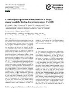
With the EGOPS software (End-to-End Generic Occultation Performance and Processing System) version 5.5 (Fritzer et al., 2009) we performed an end-to-end simulation study similar to Foelsche et al. (2008). We simulated daytime events (12:00 LT) and nighttime events (02:00 LT) for the years 2001 to 2011 via ray tracing through ionospheric and neutral atmospheric fields. We simulated the receiver height at an altitude of 800 km. In general, the orbit altitude of the GPS receiver plays a role for the magnitude of the ionospheric residual, as published by Mannucci et al. (2011). They showed that spacecrafts at higher altitudes show less residual ionospheric errors than spacecrafts at lower altitudes, comparing COSMIC orbit heights (∼ 780 km) to CHAMP (∼ 400 km). Our simulated receiver height is comparable with the COSMIC height. Hence, it shows less residual ionospheric errors due to partial cancellations of the ionospheric bending than, for example, the CHAMP satellite. The resulting phase data were used as input for standard RO retrieval of atmospheric parameters from bending angle to dry temperature. Since we focused on the separation of ionospheric errors we did not superimpose observational errors. We performed two different studies. In the first study we always employed the same atmosphere, using operational analysis fields provided by ECMWF (European Centre for Medium-Range Weather Forecasts) for all simulations, and only varied the ionosphere for each profile. The ECMWF field used in this analysis is from 1 January 2007 with T42L91 resolution. The horizontal resolution T42 corresponds to the resolution of RO data (∼ 300 km), with data available at 91 vertical levels (L91). The ionosphere was simulated with the NeUoG model (with Ne being the electron density and UoG meaning University of Graz Leitinger et al., 1995, 1997), which is driven by the F10.7 index as an indicator for the solar activity. The F10.7 index is based on the solar radio flux at a wavelength of 10.7 cm. We downloaded daily F10.7 data from the website of the National Oceanic and Atmospheric Administration, NOAA (http://www.ngdc. noaa.gov/, 2012) and calculated monthly mean values as a representative for typical solar activity, see Fig. 1. The NeUoG model provides a global 3-D electron density distribution depending on local time, season, and solar activity. The magnetic field term according to Eq. (2) is not included Atmos. Meas. Tech., 6, 2169–2179, 2013
ssion Paper
2172
J. Danzer et al.: RO residual ionospheric errors | Discussion Paper
1000
600 4
200 0 20 0
Discussion Paper
400
2 4
|
Height [km]
800
NeUoG Electron density [1011 /m3 ]
6
2
10
0
Latitude [°]
10
20
18 16 14 12 10 8 6 4 2 0
UT: 0200, Month: January, F10.7 = 140 sfu, Lon = 0.0
Fig. 1. Monthly mean solar radio flux (F10.7 index) for the years
Discussion Paper
1000
|
−22 Wm −1 Hz −1 ). for the years 2001 to 2011 (1sfu = Fig. 1. Monthly mean (F10.7 index) 2001 to 2011solar (1 sfuradio = 10flux 0−22 Wm−1 Hz−1 ).
NeUoG Electron density [1011 /m3 ]
18 16 14 12 10 8 6 4 2 0
Height [km]
Furthermore we simulated occultation events based on past realistic atmospheric fields, where the electromagnetic signal gets occulted only by the neutral atmosphere, i.e., the Atmos. Meas. Tech., 6, 2169–2179, 2013
|
in the simulations. A recent study by Liu et al. (2013) inves800 tigated to which order the ionospheric refractive index needs 2 to be considered. They compared a modified version of the 4 600 NeUoG model which included the geomagnetic term to the 6 8 10 old version without the field term (1st order approximation). 14 12 16 400 16 Their results showed no essential 12 23 effects on the bending an10 14 8 gle residuals to whether the magnetic field term is included 200 4 6 or not. 2 As an example, Fig. 2 shows typical day and night iono0 0 20 10 0 10 20 spheric conditions simulated with NeUoG. The plots show Latitude [°] the electron density distribution Ne as a function of latitude UT: 1200, Month: January, F10.7 = 140 sfu, Lon = 0.0 and height. In this particular example, the solar activity is characterized by F10.7 = 140 sfu, for January at longitude 0◦ . Fig. 2. Electron density distribution in January for F10.7 = 140 sfu As expected, the ionization level in Fig. 2 is clearly increased as a function of latitude and height, at 0◦ longitude. The top panel shows the distribution at nighttime (02:00 LT), the bottom panel during daytime (bottom panel) compared Fig. to the2. nighttime Electron density distribution in January for F10.7 = 140sfu as a function of lat shows the distribution at daytime (12:00 LT), where the electron (top panel); furthermore, there is a dependance◦ of the ionat 0 longitude. The top panelvalues shows theto distribution at night3 .time (02:00 LT), t density reaches of up 18.0 × 10¹¹ electrons/m ization on the latitude and altitude. At night there is a maxishows the distribution at day time (12:00 LT), where the electron density reaches mum around 3◦ N (top panel), while during the day there 11 are 3 18.0 ×of 10400 electrons/m . ◦ ◦ two maxima around 10 S and 18 N, at an altitude km 24simulation. We analyzed ionospheric part was ignored in that (bottom panel), illustrating the equatorial anomaly (the maxthe following questions: imum of Ne is not located at the equator, but within ±20◦ latitude of the magnetic equator). 1. How big is the contribution of the neutral atmosphere In our simulations we focused on the latitude band 20◦ S in the altitude domain where the ionospheric residual is to 20◦ N and simulated events taking place in all Januaries determined? from 2001 to 2011 at latitudes 0◦ , 5◦ S, 5◦ N, 10◦ S, 10◦ N 2. Does this contribution of the neutral atmosphere vary and at longitudes 0◦ , 60◦ E, 60◦ W, 120◦ E, 120◦ W, 180◦ E. during a solar cycle? This leads to altogether 60 simulated occultation events per year and 660 events for a period of 11 yr. This is not a repreFor that study we simulated two profiles per month (one sentative statistics, but sufficient to study the two main quesday and one night profile) for the years 2001–2009 at lontions: gitude and latitude 0◦ , which altogether makes 216 profiles. In order to study the contribution of the neutral atmosphere, 1. What are the bias characteristics of the ionosphere alone we used the ECMWF analysis field of the first day of each in the years 2001 to 2011? month at 00:00 UTC and 12:00 UTC, respectively. 2. Does, as a first test, a climatological ionospheric correc2.3 Determination of the ionospheric residual tion work on the simulated data? The residual ionospheric error was studied by analyzing the bending angle bias. At WEGC the bias is obtained by comparing the ionosphere corrected bending angle profile α www.atmos-meas-tech.net/6/2169/2013/
J. Danzer et al.: RO residual ionospheric errors
2173
with the co-located MSIS (Mass Spectrometer and Incoherent Scatter Radar) bending angle profile between 65 km and 80 km impact height (which is defined as the impact parameter minus the local radius of curvature). l 1X (αRO − αMSIS )i , bias = l i=1
(6)
where i = 1 corresponds to the first altitude level above 65 km and l is the last level below 80 km. The MSIS climatology provides atmospheric profiles depending on latitude, longitude, day of year, and universal time (or local solar time), including also dependencies on solar activity (represented by the solar radio flux F10.7 and the magnetic index Ap ) (Hedin , 1991). For our applications as a reference climatology it was modeled as a function of month, impact height, latitude, and longitude with fixed local time 0 h and fixed solar activity of F10.7 = 150 sfu and Ap = 4, so that it shows no diurnal variations and no solar variations. The reference climatology acts as a shift of the bending angle to a value around zero and will in later studies of bending angle bias differences (see Fig. 4) cancel out. We studied the daytime and nighttime bias for three different latitude zones: 60◦ S to 20◦ S, 20◦ S to 20◦ N, and 20◦ N to 60◦ N. As nighttime events we regarded RO events taking place from 02:00 to 06:00 in the morning, for the daytime bias we considered occultation events between 11:00 and 15:00, local time (LT). The time frames for the nighttime and daytime events have been chosen to allow comparisons with results by Rocken et al. (2008, 2009); Schreiner et al. (2011) who picked the same time frames. At UCAR the bending angle bias is calculated in a similar way, but in the altitude range of 60 km to 80 km. As a reference climatology they use the NCAR (National Center for Atmospheric Research) climatology (Randel et al., 2002). Hence, the absolute bias values are different for WEGC and UCAR data. We calculated the median bias of all profiles which pass quality control, within three months for CHAMP data, and within one month for COSMIC data. This leads to about 600 events (CHAMP) and about 4000 events (COSMIC), per latitude zone and daytime or nighttime event frame. CHAMP is a single satellite which performs only setting events, i.e., the satellite scans the atmosphere from top to bottom. However, COSMIC is a six satellite constellation, which measures setting as well as rising events (scanning of the atmosphere from bottom to top), leading to considerably more COSMIC RO profiles compared to CHAMP. Therefore we averaged CHAMP data over three months and took the central month as a representative for this time period, e.g., the median bias over the period March-April-May represents April.
www.atmos-meas-tech.net/6/2169/2013/
3
Results and discussion of the ionospheric residual
3.1
Satellite data results
In Fig. 3 we show the daytime (11:00–15:00 LT) and nighttime (02:00–06:00 LT) bending angle bias for 10 yr (WEGC) and 11 yr (UCAR), for three latitude zones (see Sect. 2.3). Until July 2006 we used CHAMP data for the analysis, afterwards we continued with COSMIC data, since the number of RO profiles is higher. The combination of CHAMP and COSMIC data is feasible, since the bias characteristics of both data sets are extremely similar (see Foelsche et al., 2011, and an explicit discussion below). In this 10 to 11 yr time frame the solar cycle has a maximum in the years 2001 and 2002, and a minimum in the years 2007–2009 (see Fig. 1). The negative sign of the bias is consistent with the assumption of an ionospheric origin (Sokolovskiy et al., 2009). The time series in Fig. 3 illustrates three main effects: 1. The negative bending angle bias is larger during daytime than during nighttime (diurnal cycle). 2. The daytime bending angle bias increases with solar activity, while the nighttime bias remains nearly constant (solar cycle). 3. Within a year the daytime and nighttime bending angle biases show maxima in the summer months in WEGC data (seasonal cycle). The diurnal cycle can be explained by the increase of ionization from night to day. Also the second effect reflects the change of ionization, caused by the solar cycle. Indeed we find that in the years of high solar activity the daytime bending angle bias increases in all three latitude zones. In the solar minimum years Fig. 3 shows that the WEGC as well as the UCAR bending angle data sets approach a more or less constant value. Furthermore the WEGC data sets show a seasonal dependance, reflected in the yearly peaks of the daytime and nighttime bending angle bias. The seasonal maxima depend on the latitude zone. In the extratropics maxima occur in summer: in the Northern Hemisphere in June and July (top panel of Fig. 3) and in the Southern Hemisphere in December and January (bottom panel of Fig. 3). Only the tropical zone (central panel of Fig. 3) shows no definite maxima. Finally, in the comparison of the WEGC and UCAR processed data sets we observe that the absolute bias values differ from each other. This is due to the different altitude ranges and the different reference climatologies, which are used in the calculation of the bending angle biases (see Sect. 2.3). Nevertheless, the difference between daytime and nighttime bending angle bias should be the same (1Bias = Day Bias − Night Bias) for the two data sets, if it correctly reflects the changing solar activity. This is confirmed by the results shown in Fig. 4, by comparing WEGC data (green line) and UCAR processed data (blue line). The two data sets display a very similar temporal evolution. This characteristic Atmos. Meas. Tech., 6, 2169–2179, 2013
20 20°°NN--60 60°°NN
0.0 0.0
20 20°°SS--20 20°°NN
Night, UCAR Night,UCAR UCAR Day, Day, UCAR
∆∆Bias, Bias,WEGC, WEGC, ∆∆Bias, Bias,UCAR UCAR
2020°°SS--2020°°NN
0.0 0.0
-0.4 -0.4 -0.6 -0.6
Night, WEGC Night,WEGC WEGC Day, Day, WEGC
60 60°°SS--20 20°°SS
Night, UCAR Night,UCAR UCAR Day, Day, UCAR
0.0 0.0
-0.2 -0.2
-0.4 -0.4
0.4 0.4 0.2 0.2
2 1 1 5 7 3 9 8 0 6 4 2200001 2200002 2200003 2200004 2200005 2200006 2200007 2200008 2200009 2200110 2021011
∆∆Bias, Bias,WEGC, WEGC, ∆∆Bias, Bias,UCAR UCAR
6060°°SS--2020°°SS
0.0 0.0
-0.2 -0.2
-0.4 -0.4 -0.6 -0.6 011 022 033 04 055 06 077 08 099 10 111 22000 22000 22000 220004 22000 220006 22000 220008 22000 220010 20201
bias bias characteristics characteristics over over about about one one solar solar cycle cycle for for WEGC WEGC and and UCAR UCAR bending bending angle angle data. data. From From top top canbottom be foundwe in allshow three latitude zones.the Furthermore, the bias to data from latitude zones to bottom we show data from the latitude zones difference in ◦all a constant value ◦◦ ◦◦zones approaches ◦ ◦◦ ◦◦ in ◦N,three 20 N to SS to 20 N, and SS to S. 20 Nwhich to 60 60could N, 20 20 tothat 20◦the N,seasonal and 60 60cycle toin20 20 2007, indicate Fig. S. 3
bending bending angle angle bias bias for for three three latitude latitude zones, zones, comcomparing paring WEGC WEGC (green (green line) line) and and UCAR UCAR(blue (blueline) line) 2010. Weangle find thatdata the data of thelatitude two satellites are in bending (same zone as in bending angle data (same latitude zone asgood in agreement in the overlapping period from August 2006 to Fig. 3). Fig. 3). 2008. Confirming the results of Foelsche et al. September
for WEGC data is due to the reference climatology used. The 25 similar behavior of two data sets obtained with different pro-25 cessing methods strengthens the conclusion that the observed bias difference between day and night is indeed caused by solar activity. This bending angle bias difference will therefore be used as a solar cycle dependent correction factor for the bending angle data (see Sect. 4.1). In Fig. 5 we discuss the potential impact of mixing CHAMP and COSMIC satellite data (processed at WEGC) in a 10 yr bending angle bias time series in the latitude zone 20◦ S to 20◦ N. The top plot of Fig. 5 shows again the daytime and nighttime bending angle bias characteristics, while the bottom plot shows the bending angle bias difference 1 Bias. In contrast to the previous plots we now compare the complete available WEGC data sets of CHAMP and COSMIC. CHAMP data are available from May 2001 to September 2008 and COSMIC data from August 2006 to December Atmos. Meas. Tech., 6, 2169–2179, 2013
(2011) we find very similar bias results for the two satellites. Small deviations have to be expected, since we computed monthly averages for COSMIC data, while we calculated three month averages for CHAMP, due to the smaller number of profiles – which also explains the higher variability in the CHAMP record. Finally, we conclude that Figs. 3 and 4 clearly demonstrate that despite of the ionospheric correction, which has been applied to the bending angle data (see Eq. 5), an ionospheric residual exists, which results in a negative bending angle bias. Our results are consistent with Vorobev and Krasilnikova (1994). They studied the error of the atmospheric refractive angle under different ionospheric conditions, investigating the influence of the height and thickness of ionospheric layers. They found that the atmospheric refractive recovery error (i) increases with decreasing height of the electron concentration maximum, and (ii) increases with www.atmos-meas-tech.net/6/2169/2013/
||
Fig. 4. Difference between daytime and nighttime bending angle bias for three latitude zones, comparing WEGC (green line) and UCAR (blue line) bending angle data (same latitude zone as in Fig. 4. Fig. 3). Fig. 4. Difference Difference between between day day and and night night time time
Discussion Paper Paper Discussion
Fig. 3. Nighttime and daytime bending angle bias characteristics over about one solar cycle for WEGC and UCAR bending angle data. From top to bottom we show data from the latitude zones ◦ N, 20◦ S Fig. 20◦ N 3. to to 20◦and N, andday 60◦ Stime to 20◦bending S. Fig. 3.60Night Night time time and day time bending angle angle
||
-0.6 -0.6 011 022 033 04 055 06 077 08 099 10 111 22000 22000 22000 220004 22000 220006 22000 220008 22000 220010 22001
Discussion Paper Paper Discussion
2 1 1 5 7 3 9 8 0 6 4 2200001 2200002 2200003 2200004 2200005 2200006 2200007 2200008 2200009 2200110 2200111
||
Bias [[µµrad] rad] Bias
0.2 0.2
2 1 1 5 7 3 9 8 0 6 4 2200001 2200002 2200003 2200004 2200005 2200006 2200007 2200008 2200009 2200110 2021011
-0.2 -0.2
-0.4 -0.4
0.2 0.2
0.4 0.4
Bias [[µµrad] rad] ∆∆Bias
Bias [[µµrad] rad] Bias
Night, WEGC Night,WEGC WEGC Day, Day, WEGC
-0.2 -0.2
0.4 0.4
-0.6 -0.6
2 1 1 5 7 3 9 8 0 6 4 2200001 2200002 2200003 2200004 2200005 2200006 2200007 2200008 2200009 2200110 2200111
0.0 0.0
-0.6 -0.6
0.0 0.0
Discussion Paper Paper Discussion
0.2 0.2
2020°°NN--6060°°NN
-0.4 -0.4
-0.4 -0.4
0.4 0.4
0.2 0.2
∆∆Bias, Bias,WEGC, WEGC, ∆∆Bias, Bias,UCAR UCAR
-0.2 -0.2
-0.2 -0.2
-0.6 -0.6
0.4 0.4
Bias [[µµrad] rad] ∆∆Bias
Night, UCAR Night,UCAR UCAR Day, Day, UCAR
Bias [[µµrad] rad] ∆∆Bias
0.2 0.2
Night, WEGC Night,WEGC WEGC Day, Day, WEGC
||
Bias [[µµrad]
0.4 0.4
J. Danzer et al.: RO residual ionospheric errors
Discussion Paper Paper Discussion
2174
20°S - 20°N
0.4
Night, CHAMP Day, CHAMP Night, COSMIC Day, COSMIC
-0.0
0.0
-0.3
-0.4
∆Bias [µrad]
2
200
3
200
4
200
∆Bias, CHAMP ∆Bias, COSMIC
5
200
6
200
7
200
8
200
9
200
0
201
0.2
1 201
20°S - 20°N
0.0 -0.2 -0.4
0.0
2 1 1 5 7 3 9 8 0 6 4 200 200 200 200 200 200 200 200 200 201 201
-0.2 -0.4 -0.6
Discussion Paper
0.2
1
200
Mean Value Night Profiles Mean Value Day Profiles
|
0.4
-0.4
∆Bias [µrad]
-0.6
-0.2
Discussion Paper
-0.2
-0.1
2175
|
Bias [µrad]
0.2
Bias [µrad]
0.1
Discussion Paper
J. Danzer et al.: RO residual ionospheric errors
NeUoG, Mean Value WEGC, 20°S - 20°N Neutral Atmosphere 2 1 1 5 7 3 9 8 0 6 4 200 200 200 200 200 200 200 200 200 201 201
|
Fig. 6. Top panel: mean daytime (orange line) and nighttime (blue line) bending angle bias of the simulated profiles. Bottom panel: mean bending angle bias difference (1 Bias) of the simulated pro-0.6 1 dayline), timethe(orange and satellite night time angle b 2 5 7 3 8 Fig.9 6. 0Top 1panel: mean 6 4 files (red WEGC line) processed data(blue (greenline) line) bending and 200 200 200 200 200 200 200 200 200 201 201 simulated profiles. Bottom panel: mean bending angle difference of the simulat the neutral atmosphere simulation timebias series at latitude(∆Bias) and longi(red line), processed satellite tude 0◦ (magenta line). data (green line) and the neutral atmosphere simul Fig. 5. Comparison of CHAMP and COSMIC bending anglethe biasWEGC ◦ at latitude time series based on WEGC processing. The series top panel shows and longitude 0 (magenta line). CHAMP and COSMIC daytime and nighttime bias characteristics, 27 the bottom panel displays the bias difference 1 Bias in the latitude moreon orWEGC less constant during a solar cycle (blue line), while ◦ N. CHAMP COSMIC bending angle bias time series based processzone 20◦ Sand and 20
Discussion Paper
arison of the daytime bending angle bias shows a response to the modanel shows CHAMP and COSMIC day time and night time bias characteristics, the bottom ifying solar radiation (orange line). The negative nighttime ◦ ◦ the bias difference ∆Bias in the latitude zone 20 S and 20 N.
3.2
Simulation results
In Fig. 6 we show the mean bending angle bias for simulated profiles in the tropical band. At each latitude (0◦ , 5◦ S, 5◦ N, 10◦ S, 10◦ N) we simulated profiles at longitudes 0◦ , 60◦ E, 60◦ W, 120◦ E, 120◦ W, 180◦ E. We studied the daytime (12:00 LT) and nighttime (02:00 LT) bending angle bias for the years 2001 to 2011. Thereby we always used the same ECMWF atmosphere field for all profiles and varied only the solar activity according to Fig. 1. The top panel of Fig. 6 shows the results of the mean daytime and nighttime bending angle bias characteristics. For each data point we averaged over 30 profiles. Also in the simulated case we can observe that the nighttime bias stays www.atmos-meas-tech.net/6/2169/2013/
bias fluctuates around a mean value of about −0.1 µrad, while the daytime bias changes from about −0.27 µrad to about −0.15 µrad from high to low solar activity. Following the same approach as for observational data in Fig. 4, we show in the bottom panel of Fig. 6 the bending angle bias difference between day and night (1 Bias, red line). For comparison, we show the WEGC processed observational data in the same latitude zone (20◦ S to 20◦ N, green line). One can see that the mean value of the simulated data nicely fits the observational bending angle bias difference. We do not expect full coincidence between the absolute values of the bending angle bias difference of observational and simulated data, but it is encouraging to see that the simulated results show a similar behavior: the stable nighttime bias and the solar cycle dependent daytime bias could be confirmed in the model simulation. Finally, the bottom panel of Fig. 6 also contains the simulation results of the neutral atmosphere (magenta line) at latitude and longitude 0◦ (see Sect. 2.2), using ECMWF operational analysis fields from the years 2001 to 2009. We
|
increasingly thick ionospheric layers. Our analysis confirmed their results by showing that the 26residual bias depends on the diurnal, solar and seasonal cycles. In the next subsection we address the ionospheric residual for simulated data.
Atmos. Meas. Tech., 6, 2169–2179, 2013
Discussion Paper
J. Danzer et al.: RO residual ionospheric errors 0.2
angle level, as follows:
0.0
αC0 i,SL = αCi,SL − (1BiasSL − 1BiasNeutSL ),
0.2
where αC is the original bending angle, after standard first order ionospheric correction (see Eq. 5), αC0 is the new bending angle after the additional climatological ionospheric correction, 1Bias is the bending angle difference between day and night, and 1BiasNeut is the small contribution of the neutral atmosphere in the altitude range where the bias is determined, which should not be corrected. The subscript i indicates that the bending angles αC and αC0 are vectors depending on the impact height. The subscript L denotes the latitude zone in which the occultation event takes place. Finally, the subscript S stands for the point in time of the solar cycle. Hence, we subtract a correction factor from a daytime bending angle profile, which magnitude depends on the phase of the solar cycle and the latitude zone in which the occultation event takes place. Furthermore we subtract the small neutral atmospheric contribution from the correction factor. A first test of this approach is presented in the next section.
NeUoG: Lat 0°, Lon 0° - - Corrected Bending Angle
0.6
2 1 1 5 7 3 9 8 0 6 4 200 200 200 200 200 200 200 200 200 201 201
0.2
Discussion Paper
0.4
0.8
(7)
|
∆Bias [µrad]
2176
|
∆Bias [µrad]
0.2 0.4
NeUoG: Lat 5°S, Lon 0° - - Corrected Bending Angle
0.6
2 1 1 5 7 3 9 8 0 6 4 200 200 200 200 200 200 200 200 200 201 201
4.2
Model results on the reduction of the systematic residual ionospheric error |
0.8
Discussion Paper
0.0
Discussion Paper
Fig. 7. Bending angle bias difference (1Bias) between day and As the next step we used the simulated profiles to perform night for latitude 0◦ (top panel) and 5◦ S (bottom panel) for the a first test of the newly introduced climatological ionospheric month January from 2001–2011. The solid blue lines show the ◦ Bending angle bias angle difference (∆Bias)for between and night for latitude 0correction. (top panel) Weand tested the performance of the correction over bending bias difference originalday bending angle data sets, ttom panel) the for dashed the month January from 2001 to 2011. The solid blue lines show the bending a solar cycle on two different geographic locations (at latigreen lines show the data after climatological iono◦ S, both at longitude 0◦ ). ias difference for original bending angle data sets, the dashed green lines show data5after spheric correction. tudethe 0◦ and
ogical ionospheric correction.
|
The correction factor we used is the mean bending angle bias difference (1 Bias) of all simulated profiles (red line of bottom panel of Fig. 6). From this mean bending angle bias difference we subtracted the contribution of the neutral atmosphere (1BiasNeut ). Since we used the same ECMWF analysis field (1 January 2007) for every profile simulated with ionosphere, in our special case we always subtracted the same neutral atmospheric contribution (1BiasNeut ) from our bending angle bias difference (1 BiasSL ). For this particular day 1BiasNeut amounts to 1.8 × 10⁻⁸ rad. The next step is to correct the daytime bending angle αC with this mean bending angle bias difference according to Eq. (7), i.e., the whole profile is shifted by the same correction factor. As explained in Sect. 4.1, the magnitude of the correction factor depends on the latitude zone and the phase of the solar cycle. This leads to a larger correction factor in times of high solar activity and a smaller factor in times of low solar activity. Figure 7 illustrates the daytime to nighttime bending angle bias difference before (blue solid lines) and after (green dashed lines) the climatological ionospheric correction. The top plot shows the bias difference for the latitude 0◦ , the bottom plot for 5◦ S. As expected, the 0◦ and 5◦ S bending angle profiles show a smaller daytime to nighttime bending angle bias difference after the correction (see dashed lines of Fig. 7). There is still a dependance of the bias difference on the solar radiation, but the residual is clearly reduced.
28 simulated the pure effect of the neutral atmosphere without ionosphere, because we wanted to provide an estimate of the contribution of the neutral atmosphere to the bending angle bias between 65 and 80 km. Furthermore we wanted to study if this contribution shows a dependance on the solar cycle. We observed that the contribution of the neutral atmosphere stays stable during a solar cycle, resulting in a 1 Bias that fluctuates around a mean value of −0.006 µrad. At least in the ECMWF analysis fields, the contribution of the neutral atmosphere is small and almost constant.
4 4.1
Climatological ionospheric correction A simple bending angle correction factor
Now we want to introduce an idea for a simple correction of the ionospheric residual, which has been identified in Sect. 3. Based on the results of Sect. 3 we identify the difference between daytime and nighttime bias as a good indicator for the ionospheric residual. Since the residual depends on latitude and on the phase of the solar cycle, we propose a correction of the daytime profiles, which is applied at bending Atmos. Meas. Tech., 6, 2169–2179, 2013
www.atmos-meas-tech.net/6/2169/2013/
Discussion Paper
35January - Diff to ECMWF Temp 35January - Diff to ECMWF Temp
The temperature plots (top row) show the typical behavior of low latitude profiles with a pronounced tropopause and stratopause and the influence of ionospheric errors at high altitudes. The ionospheric residual is clearly reduced after the climatological ionospheric correction (right panel), which becomes even more evident when looking at the difference plots (bottom row). These plots illustrate how the temperature errors increase with altitude and solar activity, resulting in a fan like distribution, with maximum spread at high altitudes. As an example, January 2002 has the highest F10.7 value (226.8 sfu), see Fig. 1, and shows a maximum difference of about −3.9 K at 35 km altitude. For a solar minimum year on the other hand, as e.g., 2008 (F10.7 = 75.3 sfu), the temperature bias reduces to a value of −1.4 K. Studying the corrected data sets, we find that the temperature profile of January 2002 shows a difference of about −1.0 K at 35 km altitude, while for 2008 it amounts to 0.4 K. As a result of the correction the spread of the fan is clearly reduced and even more important, it is centered around zero with maximum absolute deviations of less than about 1.0 K.
Discussion Paper
80 January - Temperature 80 January - Temperature 70 70 2001 C 60 2002 60 2001, 2002, C 2003 2003, C 50 2004 50 2004, C 2005 2005, C 2006 C 40 2007 40 2006, 2007, C 2008 2008, C 30 2009 30 2009, C 2010 2010, C 20 2011 20 2011, C ECMWF Temp ECMWF Temp 10 10 180 200 220 240 260 280 180 200 220 240 260 280 T [K] T [K]
2177
|
Altitude [km]
J. Danzer et al.: RO residual ionospheric errors
|
Altitude [km]
25 20 15
2001 2002 2003 2004 2005 2006 2007 2008 2009 2010 2011
30 25 20 15
2001, C 2002, C 2003, C 2004, C 2005, C 2006, C 2007, C 2008, C 2009, C 2010, C 2011, C
5
Summary, conclusions, and outlook
|
10 4 3 2 1 0 1 2 3 10 4 3 2 1 0 1 2 3 ∆ T [K] ∆ T [K]
Discussion Paper
30
Discussion Paper
For the study of neutral atmospheric parameters based on ra-
dio occultation (RO) data it is important to correct for the Fig. 8. Top panels: dry temperature versus altitude for January procontribution of the ionosphere. The commonly applied linfiles from 2001–2011, before (left) and after (right) climatological ear ionospheric correction is based on the fact that the ionoionospheric correction of bending angles. Bottom panels: dry temp panels: dry temperature versus toaltitude for January profiles to 2011, before medium. A combination of the two perature difference relative the ECMWF temperature up to 35from km, 2001 sphere is a dispersive again before (left) and after (right) correction. All profiles generated fter (right) climatological ionospheric correction of bending angles. Bottom panels: dry GPS frequencies leads to an ionospheric correction to first latitude and longitude 0◦ . temperature up to 35km, again before order.(left) Sinceand thisafter correction is an approximation, there exists differenceatrelative to the ECMWF
ection. All profiles generated at latitude and longitude 0◦ .
|
an ionospheric residual, depending on the change of the solar activity. This residual results in a systematic ionospheric error, which affects the accuracy of the atmospheric parameters, also at low altitudes. We studied this systematic ionospheric residual by analyzing the bending angle bias characteristics of CHAMP and COSMIC RO data from the years 2001 to 2011. We confirmed that the nighttime bending angle bias stayed constant over the whole period of 11 yr, while the daytime bias increases from low to high solar activity. As a result, the difference between nighttime and daytime bias increases from about −0.05 µrad to about −0.4 µrad. Thus the average daytime bending angles under solar maximum conditions are approximately 0.35 µrad smaller than during low solar activity. When studying short-term atmospheric trends over an unfavorable time interval (i.e., from low to high solar activity or vice versa) the residual ionospheric error could lead to a trend, which could wrongly be interpreted as an anthropogenically induced atmospheric trend. Since absolute bending angle values decrease exponentially with altitude, the importance of this residual error increases with altitude. Ringer and Healy (2008) studied projected bending angle trends based on a climate model run. At an impact altitude of 26 km, e.g., they report a positive trend of about 4 µrad per
Next we studied if this reduction of the bending angle 29 bias also results in a bias reduction of the derived parameter dry temperature. The results for 0◦ and 5◦ S are very similar, Fig. 8 shows those for 0◦ as a representative example. We cut the profiles below 10 km altitude, since here the difference between dry and physical temperature becomes important, which is not the focus of this study. In Fig. 8 we show the daytime (12:00 LT) January dry temperature profiles for the years 2001–2011. Besides being an important parameter for climate research, temperature profiles are of special interest, since they illustrate how the ionospheric error amplifies through the retrieval (Schreiner et al., 2011). The top row shows dry temperature profiles up to 80 km altitude and the “true” ECMWF temperature profile (dashed red line), which has been used as input for the simulation. The bottom row of the figure displays the temperature difference of each profile to this ECMWF profile, in the altitude range up to 35 km, where RO profiles are frequently used for climatological studies. The left panels of Fig. 8 show the original temperature profiles, while the right panels show the results after the climatological ionospheric correction, marked with a capital C. www.atmos-meas-tech.net/6/2169/2013/
Atmos. Meas. Tech., 6, 2169–2179, 2013
2178 decade. The trend decreases to about 1.2 µrad per decade, at an impact height of 30 km, see Fig. 1 in Ringer and Healy (2008). Depending on the altitude considered, the residual ionospheric error could therefore range from a few percent up to an important fraction of a short-term bending angle trend. As the next step we simulated RO profiles at tropical latitudes. The goal was, on the one hand, to study separately the influence of the ionosphere and the neutral atmosphere. On the other hand, we wanted to test a first approach to reduce the ionospheric residual and the systematic error in the atmospheric parameters. First of all, our analysis showed that the contribution of the neutral atmosphere at the altitude where the bending angle bias was determined (65 km to 80 km) is small and almost constant with time. Second, by investigating retrieved dry temperature profiles, we studied the influence of the ionosphere on neutral atmosphere RO data. As expected, the influence increases with solar activity and altitude. As an example, the simulated January profiles at a latitude and longitude of 0◦ show a maximum bias of −3.9 K (2002, high solar activity) and a minimum bias of −1.4 K (2008, low solar activity) at 35 km altitude. In this simulation we also tried to reduce the ionospheric residual of the simulated profiles. The principle idea was to use the bending angle bias characteristics of a solar cycle (11 yr) and to correct the daytime bending angle by this factor, depending on the latitude and the phase of the solar cycle. Discussing the same example as before, we found that the climatological ionospheric correction reduces the error spread at 35 km altitude from 2.5 K to 1.7 K, while the maximum absolute errors stay below about 1.0 K. These results confirm, that the proposed approach of correcting the daytime bending angle profiles by a solar activity dependent factor, works in principle. We note that an unknown, but apparently time constant, nighttime bias will remain in the corrected data. For a detailed formulation of the climatological ionospheric correction, which can be applied to observational data, it will be important to include multi-satellite RO results from the currently evolving solar maximum, since results from the last maximum are only based on RO data with comparatively high noise level from a single-satellite mission (CHAMP). In a first step, the correction of observational satellite data, will be based on COSMIC RO data only, and no mixing of satellite data will take place. However, when we include different satellites we will regard their orbit altitudes as a further factor in our correction (Mannucci et al., 2011). Furthermore, a fine tuning of the applied correction will comprise a detailed study of the local time dependance of the ionospheric residual and an optimized formulation of the geographic dependance, where we will also consider if magnetic coordinates are better suited than geographic coordinates. Another aspect, which has to be considered, is the contribution of the neutral atmosphere to the bending angle above 65 km altitude, where the bending angle bias is operationally determined in our retrieval. We have to make sure that we Atmos. Meas. Tech., 6, 2169–2179, 2013
J. Danzer et al.: RO residual ionospheric errors do not remove an apparent ionospheric bias, which is indeed a real contribution of the neutral upper atmosphere – which also shows changes caused by the solar cycle. Our preliminary analysis based on ECMWF data indicated that this effect is small and almost constant with time, but further work is needed to confirm these results. A simple approach to minimize this potential problem could be to increase the minimum altitude of the range, where the bending angle bias is determined (e.g., from currently 65 km to 70 km), which would significantly reduce any contribution from the neutral atmosphere. Finally, we want to emphasize that the goal of the proposed correction is not to improve individual profiles, but to reduce the small ionospheric residual in large ensembles of RO data for climate applications. A further advantage of the new approach is that it is model independent, based purely on observational RO data. Acknowledgements. We are grateful to the UCAR/CDAAC and WEGC GPS RO operational team members for their contributions in OPS system development and operations. Furthermore we thank ECMWF for providing analysis data. Our work was funded by the Austrian Science Fund (FWF) under grant P22293-N21 (BENCHCLIM project). Finally we thank G. Kirchengast (WEGC) for fruitful discussions and M. Schw¨arz (WEGC) for his technical support. Edited by: S. Buehler
References Bassiri, S. and Hajj, G. A.: Higher-order ionospheric effects on the GPS observables and means of modeling them, Manuscr. Geod., 18, 280–289, 1993. Budden, K. W.: The Propagation of Radio Waves, Cambridge University Press, Cambridge, New York, 1985. Fjeldbo, G., Kliore, A. J., and Eshleman, V. R.: The neutral atmosphere of Venus as studied with the Mariner V radio occultation experiments, Astron. J., 76, 2, 123–140, doi:10.1086/111096, 1971. Foelsche, U., Kirchengast, G., Steiner, A. K., Kornblueh, L., Manzini, E., and Bengtsson, L.: An observing system simulation experiment for climate monitoring with GNSS radio occultation data: setup and testbed study, J. Geophys. Res., 113, D11108, doi:10.1029/2007JD009231, 2008. Foelsche, U., Scherllin-Pirscher, B., Ladst¨adter, F., Steiner, A. K., and Kirchengast, G.: Refractivity and temperature climate records from multiple radio occultation satellites consistent within 0.05 %, Atmos. Meas. Tech., 4, 2007–2018, doi:10.5194/amt-4-2007-2011, 2011. Fritzer, J., Kirchengast, G., and Pock, M.: End-to-End Generic Occultation Performance Simulation and Processing System Version 5.5 (EGOPS5.5) Software User Manual, University of Graz, Austria, WEGC and IGAM, WEGC–EGOPS–2009–TR01, version 1, 2009. Gobiet, A. and Kirchengast, G.: Advancements of GNSS radio occultation retrieval in the upper stratosphere for opti-
www.atmos-meas-tech.net/6/2169/2013/
J. Danzer et al.: RO residual ionospheric errors mal climate monitoring utility, J. Geophys. Res., 109, D24110, doi:10.1029/2004JD005117, 2004. Hajj, G. A., Kursinski, E. R., Romans, L. J., Bertiger, W. I., and Leroy, S. S.: A technical description of atmospheric sounding by GPS occultation, J. Atmos. Solar-Terr. Phys., 64, 451–469, doi:10.1016/S1364-6826(01)00114-6, 2002. Hardy, K. R., Hajj, G. A., and Kursinski, E. R.: Accuracies of atmospheric profiles obtained from GPS occultations, Int. J. Satell. Commun., 12, 463–473, doi:10.1002/sat.4600120508, 1994. Hedin, A. E.: Extension of the MSIS thermosphere model into the middle and lower atmosphere, J. Geophys. Res. 96, A2, 1159– 1172, doi:10.1029/90JA02125, 1991. Ho, S.-P., Kirchengast, G., Leroy, S., Wickert, J., Mannucci, A. J., Steiner, A. K., Hunt, D., Schreiner, W., Sokolovskiy, S., Ao, C., Borsche, M., von Engeln, A., Foelsche, U., Heise, S., Iijima, B., Kuo, Y.-H., Kursinski, E. R., Pirscher, B., Ringer, M., Rocken, C., and Schmidt, T.: Estimating the uncertainty of using GPS radio occultation data for climate monitoring: intercomparison of CHAMP refractivity climate records from 2002 to 2006 from different data centers, J. Geophys. Res., 114, D23107, doi:10.1029/2009JD011969, 2009. Kedar, S., Hajj, G. A., Wilson, B. D., and Heflin, M. B.: The effect of the second order GPS ionospheric correction on receiver positions, Geophys. Res. Lett., 30, 1829, doi:10.1029/2003GL017639, 2003. Kuo, Y. H., Wee, T. K., Sokolovskiy, S., Rocken, C., Schreiner, W., Hunt, D., and Anthes, R. A.: Inversion and error estimation of GPS radio occultation data, J. Meteor. Soc. Jpn., 82, 507–531, 2004. Kursinski, E. R., Hajj, G. A., Schofield, J. T., Linfield, R. T., and Hardy, K. R.: Observing Earth’s atmosphere with radio occultation measurements using the Global Positioning System, J. Geophys. Res., 102, 23429–23465, 1997. Ladreiter, H. P. and Kirchengast, G.: GPS/GLONASS sensing of the neutral atmosphere: model-independent correction of ionospheric influences, Radio Sci., 31, 877–891, doi:10.1029/96RS01094, 1996. Leitinger, R. and Kirchengast, G.: Easy to use global and regional models – a report on approaches used in Graz, Acta Geod. Geophys. Hung., 32, 329–342, 1997. Leitinger, R., Titheridge, J. E., Kirchengast, G., and Rothleitner, W.: A “simple” global empirical model for the F layer of the ionosphere, University Graz, Wiss. Bericht 1/1995IMG, 1995. Liu, C. L., Kirchengast, G, Zhang, K. F. , Norman, R., Li, Y., Zhang, S. C., Carter, B., Fritzer, J., Schwaerz, M., Choy, S. L., Wu, S. Q. , and Tan, Z. X.: Characterisation of Residual Ionospheric Errors Using GNSS RO, revised manuscript Adv. Space Res., 52, 821–836, 2013. Mannucci, A. J., Ao, C. O., Pi, X., and Iijima, B. A.: The impact of large scale ionospheric structure on radio occultation retrievals, Atmos. Meas. Tech., 4, 2837–2850, doi:10.5194/amt-42837-2011, 2011. Melbourne, W. G., Davis, E. S, Duncan, C. B., Hajj, G. A., Hardy, K. R., Kursinski, E. R., Meehan, T. K., Young, L. E., and Yunck, T. P.: The application of spaceborne GPS to atmospheric limb sounding and global change monitoring, JPL Publ., 94, 147 pp., 1994.
www.atmos-meas-tech.net/6/2169/2013/
2179 Petrie, E. J., Hern´andez-Pajares, M., Spalla, P., Moore, P., and King, M. A.: A review of higher order ionospheric refraction effects on dual frequency GPS, Surv. Geophys., 32, 197–253, 2011. Pirscher, B.: Multi-satellite climatologies of fundamental atmospheric variables from radio occultation and their validation, Ph.D. thesis, Wegener Center Verlag Graz, Austria, ISBN 9783-9502940-3-3, Sci. Rep. 33-2010, 2010. Randel, W., Chanin, M. L., and Michaut, C.: SPARC intercomparison of middle atmosphere climatologies, SPARC, WCRP 96, WMO/TD No. 1142; SPARC Report No. 3, 2002. Ringer, M. A. and Healy, S. B.: Monitoring twenty-first century climate using GPS radio occultation bending angles, Geophys. Res. Lett., 35, 5, 2008. Rocken, C., Schreiner, B., Sokolovskiy, S., Hunt, D., and Syndergaard, S.: Formosat-3/COSMIC, The Ionosphere as Signal and Noise, Space Weather Workshop, Boulder, CO, USA, 2008. Rocken, C., Schreiner, W., Sokolovskiy, S., and Hunt, D.: Ionospheric errors in COSMIC radio occultation data, paper presented at the 89th American Meteorological Society Annual Meeting, Phoenix, AZ, USA, 2009. Schreiner, B., Sokolovskiy, S., Hunt, D., Ho, B., and Kuo, B.: Use of GNSS Radio Occultation data for Climate Applications, presentation at the World Climate Research Programme (WCRP) workshop, Denver, CO, USA, 2011. Smith, E. and Weintraub, S.: The constants in the equation for atmospheric refractive index at radio frequencies, Proc. IRE, 41, 1035–1037, 1953. Steiner, A. K., Kirchengast, G., Lackner, B. C., Pirscher, B., Borsche, M., and Foelsche, U.: Atmospheric temperature change detection with GPS radio occultation 1995 to 2008, Geophys. Res. Lett., 36, L18702, doi:10.1029/2009GL039777, 2009. Sokolovskiy, S., Schreiner, W., Rocken, C., and Hunt, D.: Optimal noise filtering for the ionospheric correction of GPS radio occultation signals, J. Atmos. Ocean. Tech., 26, 1398–1403, doi:10.1175/2009JTECHA1192.1, 2009. Spilker, J. J.: Signal structure and performance characteristics, in: Global Positioning System, edited by: Janiczek, P. M., papers published in Navigation, 1, Institute of Navigation, Washington, DC, USA, Berlin, New York, 29–54, 1980. Syndergaard, S.: On the ionosphere calibration in GPS radio occultation measurements, Radio Sci., 35, 865–883, 2000. Vergados, P. and Pagiatakis, S.: Latitudinal, solar, and vertical variability of higher-order ionospheric effects on atmospheric parameter retrievals from radio occultation measurements, J. Geophys. Res., 116, A09312, doi:10.1029/2011JA016573, 2011. Vorob’ev, V. V. and Krasil’nikova, T. G.: Estimation of the accuracy of the atmospheric refractive index recovery from Doppler shift measurements at frequencies used in the NAVSTAR system, Izv. Atmos. Ocean. Phys., 29, 602–609, 1994.
Atmos. Meas. Tech., 6, 2169–2179, 2013