THOMAS BANCHOFF AND FRANK FARRIS. For a compact oriented ... been developed and generalized in papers of Webster [Wl], [W2], and employed as a ...
PACIFIC JOURNAL OF MATHEMATICS Vol. 161, No. 1, 1993
TANGENTIAL AND NORMAL EULER NUMBERS, COMPLEX POINTS, AND SINGULARITIES OF PROJECTIONS FOR ORIENTED SURFACES IN FOUR-SPACE THOMAS BANCHOFF AND FRANK FARRIS For a compact oriented smooth surface immersed in Euclidean four-space (thought of as complex two-space), the sum of the tangential and normal Euler numbers is equal to the algebraic number of points where the tangent plane is a complex line. This follows from the construction of an explicit homology between the zero-chains of complex points and the zero-chains of singular points of projections to lines and hyperplanes representing the tangential and normal Euler classes.
1. Introduction. For a compact two-dimensional surface smoothly immersed in Euclidean four-dimensional space R4 , also thought of as complex two-dimensional space C 2 , the sum of the Euler number of M and the Euler number of its normal bundle is the negative of the algebraic number of (isolated) complex points where its tangent plane is the graph of a complex linear function. Our aim in this article is to present a geometric proof of this theorem. This theorem, already implicit in the fundamental paper of Chern and Spanier [C-S], has been developed and generalized in papers of Webster [Wl], [W2], and employed as a lemma in a number of other investigations, for example the work of Hoffman and Osserman [H-O] and Fiedler [F]. These papers rely on a variety of abstract techniques from algebraic topology and differential geometry, and it is frequently not easy to see the underlying geometric content of the theorem. In this paper, we present a concrete proof of the theorem for oriented surfaces, by interpreting the Euler numbers as singularities of projections in order to obtain 0-chains representing the Poincare duals of the tangential and normal Euler classes, and by using the Gauss map of the surface to exhibit an explicit homology between these chains and the 0-chain of (indexed) complex points. Consider briefly the Euler numbers involved in the theorem. The (tangential) Euler number of M is the most well-known topological invariant of an oriented surface, characterized by a theorem of Heinz;
2
THOMAS BANCHOFF AND FRANK FARRIS
Hopf as the algebraic sum of the zeros of a field of vectors tangent to M . In terms of singularities of projections, the Euler number is the number of maxima plus the number of minima minus the number of ordinary saddle points for a generic real-valued function on the surface, i.e. a projection of the surface into a line. Similarly the normal Euler number of an immersion of a surface into R4 can be defined as the algebraic sum of the zeros of a field of vectors normal to M. If at each point of M, we construct a normal vector field by taking the normal component of the fixed unit vector v, then this normal vector field is zero precisely at the points of M where v is contained in the tangent plane, so the projection into the three-dimensional hyperplane perpendicular to v has a singularity at p . Thus in terms of singularities of projections, we may express the normal Euler number as the algebraic number of singularities of a projection of M into a hyperplane. What is the relationship between these two Euler numbers? It is surprising that the sum of the tangential and the normal Euler numbers has anything to do with the algebraic number of points at which the tangent plane to M is a complex line, but that is precisely the content of the theorem. To help to understand this relationship, we turn to the Gauss map of the immersion. If X: M2 —• R4 is a smooth immersion of an oriented two-dimensional manifold into Euclidean four-space, then translating the tangent plane of M2 to the origin induces a map, GX, from M2 to (7(2, 4), the Grassmann manifold of oriented two-planes in four-space, also called the Grassmannian. We will show that the three terms in the theorem count the algebraic number of intersections of the image of the Gauss map of M with certain surfaces in the Grassmannian. We will show that these surfaces form the boundary of a three-dimensional chain in (7(2, 4), and the intersection of this chain with the Gauss map of the surface provides an explicit homology among the 0-chains that represent the three terms in the equation. We begin with an expanded discussion of the Euler numbers in question, interpreting them for curves and surfaces in Euclidean twoand three-dimensional space to indicate the geometric nature of the approach we take to prove the theorem. We then present a detailed tour of the Grassmann manifold (7(2, 4). With this background, we present several examples illustrating the various concepts, leading up to our proof of the theorem. 2. Euler numbers and singularities of projections. In general, the concept of a characteristic class of a vector bundle is quite abstract;
TANGENTIAL AND NORM EULER NUMBERS AND COMPLEX POINTS
3
the most common approaches are axiomatic, covering the most general situation [M-S]. But in the case of a submanifold immersed in a Euclidean space, these abstract concepts can be viewed concretely in terms of the singularities of projections into lower-dimensional subspaces. (See [C] and [B-McC] for examples of this approach.) 2A. A simple closed curve. Our most elementary example is a smooth embedding of the circle as a simple closed curve in the Euclidean plane with a finite number of inflection points. Associated with any unit vector v is the height function obtained by projecting the curve into the line along v. The critical points of this height function are the points where the vector tangent to the curve is perpendicular to v. For almost any v, this height function has finitely many critical points on the curve, an even number of them, alternately maxima and minima as we proceed around the circle. (If this is not true for a particular v, we may rotate the curve slightly and obtain a curve that does have the property with respect to v.) We can interpret these properties by using the Gauss map GX of the embedding X, which sends each point of the (counterclockwise oriented) circle to the unit tangent vector to the curve at the point, translated to the origin. Thus the Gauss map GX goes from the circle to the circle. If we project, for instance, to the line along the second standard basis vector β2, then the critical points are the points with unit tangent vector ± e i . We can index a critical point by - 1 if the Gauss map crosses from below the ei-axis to above and + 1 if it crosses from above to below. The points with their Gauss image in the upper semi-circle form a collection of curves on the original circle, each one beginning with a - 1 critical point and ending with a critical point indexed + 1 . This collection of arcs on the circle provides an explicit homology between the positive and negative points. Next suppose we consider another direction, v, on the unit circle. As in the case of β2, we may index the points where the tangent vector is perpendicular to v to obtain another 0-chain. We claim that this 0chain is homologous to the one obtained for β2. To obtain an explicit homology, we consider an arc of vectors v(ί) on the unit circle going from v(0) = β2 to v(l) = v. As t changes from 0 to 1, the critical points for the projection to v(ί) trace out a collection of curves on the original circle. As we pass a vector parallel to the tangent line at an inflection point of the curve, two critical points will coalesce into one, or a pair of critical points will arise spontaneously from a single point. In any case, the critical points at the beginning together with
THOMAS BANCHOFF AND FRANK FARRIS
FIGURE
la
FIGURE
FIGURE
lc
FIGURE Id
lb
those at the end form the boundary of a collection of oriented curves; these arcs traced on the circle exhibit an explicit homology between the two sets of critical points. (See Figures la, lb, lc, and Id.) In this rather elementary example, we see that the signs of the critical points sum to zero for almost any projection to a line along a unit vector, and that the 0-chains corresponding to projections to two diίFerent directions are homologous by an explicit homology obtained from the Gauss mapping. The same results are true for a curve immersed in the plane, or for that matter in n-dimensional space R" . 2B. The Euler number of a compact surface in R 3 . For a more complicated example, consider a generic immersion of an oriented smooth surface without boundary into Euclidean three-space
TANGENTIAL AND NORM EULER NUMBERS AND COMPLEX POINTS 2
3
5
X: M -* R . As above, we wish to show how to determine its (tangential) Euler number by using the Gauss map GX which sends each point p of M to the oriented plane through the origin parallel to the tangent plane to the surface of the point. Following the usual practice, we identify an oriented plane with the unit normal perpendicular to the oriented tangent plane to X(M) at X(p), so the image of GX 3 lies on the unit sphere in R . The direction of the unit normal is chosen such that the orientation of the tangent plane followed by the 3 unit normal gives the orientation of all of R . To calculate the tangential Euler number, we consider the zeros of a tangential vector field, for example the field that assigns to p the projection to the third coordinate vector e3 into the tangent plane at X(p). This vector field is zero exactly when the projection to the line of e$ is singular, that is, when the tangent plane at X{p) is perpendicular to e$. This happens when the image of the Gauss map at p is either e3 or - e 3 , the north or south pole of the unit sphere S2. We assume that for the surface X(M), each point p in the preimage of ±β3 under GX will have a disc neighborhood on which the Gauss map is one-to-one. (If this is not true, then we may rotate the surface slightly in almost any direction and this property will hold.) Following Gauss's original definition, we assign the index 1 to p if the Gauss map in a neighborhood of p is orientation-preserving and - 1 if it is orientation-reversing. The plus sign identifies the points which are maxima or minima of the projection of the surface to the third coordinate axis, and the minus sign identifies the ordinary saddle points. The nature of the critical points can be determined by expressing the surface in the neighborhood of a critical point as the graph of a function (x,y9 fix, y)). Then the index of the critical point is 1 or - 1 depending on the algebraic sign of the Hessian fxxfyy - f2y. The sum of the indices of these points is called the (tangential) Euler number of M. More formally, this indexed set of critical points is defined to be the Poincare dual of the tangential Euler class of M. To see that the Euler number and the Euler class are well-defined, we choose another unit vector v and consider the 0-chain of indexed critical points for the projection of the surface to the line along v. For most directions v, the minor arc v(ί) of unit vectors on the sphere from v(0) = β3 to v(l) = v will meet the image of the Gauss map of the surface "transversely" so that as we move from v(0) to v(l), the indexed critical points of the projection to v(ί) trace curves on M, with a finite number of exceptional positions where a maximum
6
THOMAS BANCHOFF AND FRANK FARRIS
or minimum coalesces with a saddle, or where a saddle and a local extremum arise instantaneously. In any case, the 0-chain at the end minus the 0-chain at the beginning is the boundary of an explicitly constructed oriented 1-chain, so these 0-chains represent the same 0dimensional homology class, the tangential Euler class, and the sum of their indices is a well-defined integer, the (tangential) Euler number, denoted by χ(M). A similar argument shows that these same results are true for a surface immersed in ^-dimensional space, although the nature of the Gauss map is more complicated in higher dimensions (see below). The process used in this example illustrates the kind of argument we will use in the proof of the theorem. 2C. The normal Euler number of an immersed surface in R 4 . For an immersion X: M —• R 4 , a theorem of Whitney [Wh] states that the sum of the indices of the zeros of any generic normal vector field will be independent of the field used to define it, and this common value is defined to be the normal Euler number of the immersion. As in the case of the tangential Euler number, we may approach the normal Euler number in terms of singularities of projections. One way to obtain a normal vector field on an immersed surface is to start with a fixed unit vector v and consider the projection Np\ of v into the normal space t o M a t p . The zeros of this vector field will occur precisely at the points p where the vector v lies in the tangent space at p, and for almost all v, there will be a finite number of such singular points p. If we project down v into the three-dimensional subspace perpendicular to v, then the zeros of Np\ are characterized by the fact that the image of the tangent space at X(p) has dimension less than two. In the generic situation, this will happen only at a finite number of points, and the rank at each of these singular points is one. In three-dimensional space, we can recognize such singularities by the fact that the image of the surface has a "pinch point" or "Whitney umbrella point", where the image of the tangent plane to the surface in R 4 is just a line in R 3 . It is possible to assign to each of these pinch points an index 1 or - 1 to obtain a 0-chain Z(v). For almost any other unit vector w, all but a finite number of points on the arc y(t) from v(0) = v tov(l) = w will have generic pinch points as their singularities, and the pinch points of \(t) will trace out a collection of arcs on M. At the singular positions, two pinch points coalesce and disappear or two new pinch points arise instantaneously. This collection of arcs gives an explicit homology between the 0-chains for v(0)
TANGENTIAL AND NORM EULER NUMBERS AND COMPLEX POINTS
7
and v(l), so the homology class of the 0-chain Z(v) is independent of the direction v used to define it. This integral homology class is called the normal Euler class, and the sum of the indices of the pinch points will be a well-defined number, n(X), the normal Euler number of the immersion. Although the tangential Euler number can be determined using any immersion whatsoever, the normal Euler number depends on the im4 4 4 mersion into R . In particular, if F: R —• R is reflection in any hyperplane, then n(FoX) = -n(X). We will use this fact in our later constructions. We also mention a theorem of Whitney [ Wh] which we will not use in the proof but which will play a role in the analysis of the examples: If X is a smooth embedding of an orientable surface into R 4 , with no self-intersection points, then n(X) — 0. In the case that X is an immersion with a finite number of transverse intersections, then n(X) is given by the algebraic number of intersection points. In particular, if there is only one such self-intersection point, then n(X) = ±2. 2D. Elementary examples. A surface immersed in X: M2 -» R 3 is automatically immersed in R 4 , and the projection into the hyperplane R 3 is just X itself so it has no singularities. Thus the normal Euler number is 0, even though the tangential Euler number will not be zero for any orientable surface other than the torus. Thus in general χ{M)φn{X). To measure the difference between the tangential and normal Euler numbers, we appeal to the "complex points" of X(M) in R 3 thought of as a hyperplane in C 2 . A complex line is the graph of a complex linear mapping, z = x + yi-+w = (a + bi)z + (c + dϊ) = (a + bi)(x + yί) + (c + di) = (ax - by + c) + (bx + ay + d)ί. In real coordinates, this graph is given by (A: , y, ax - by + c, bx + ay + d). The only plane in R 3 that can be represented in this way must have bx+ay+d = 0 for all x, y so a = b — d = 0. Thus the only complex lines in R 3 are the horizontal planes (JC , y, c, 0). We already know that the tangential Euler number of M can be expressed as the sum of indices associated to the points where the tangent plane is horizontal, perpendicular to e^, and in the case of an immersion to R 3 , these are exactly the complex points, where the tangent plane is a complex line. We shall see that this relationship holds even when an immersion of M into R 4 is not contained in a hyperplane. To see when the tangent plane at a point is a complex line, it is convenient to use the properties of a linear transformation of R 4
8
THOMAS BANCHOFF AND FRANK FARRIS 2
known as the / homomorphism. Multiplication by / in C sends the vector (x + yί, u + vi) to (—y + xi, -v + uί). This motivates the definition J(x, y, u, v) = (—y, x, — υ , u). We observe that if a two-dimensional plane through the origin is given by the graph of a linear function (x, y, mx + ny, px + qy), then this plane will be preserved under the action of / if and only if
J(x, y, mx + ny, px + qy) = (-y, x, -px - qy, mx + ny) satisfies the same linear equations, namely — px — qy = m(—y) + nx and mx + ny = p(—y) + qx for all x and y. This will happen only when n — —p and m = q , so the mapping is (x, y, mx + ny, —nx + my). This map corresponds in complex notation to the graph of the complex linear function z —• z(m - nί). Another important example of an orientable surface in 4-space is the flat torus T2, obtained by mapping the point (s, t) in the square domain ( 0 < s < 2 π , 0 < t < 2π) to the point X(s, t) = (cos(.s), sin(s), cos(^), sin(ί)). The plane through the origin parallel to the tangent plane at a point X(s, t) is given by linear combinations of the partial derivative vectors Xs(s, t) = (-sin(s), cos^), 0, 0) and Xt(s, t) = (0, 0, -sin(ί), cos(0). But then JXs(s, t) = (-cos(s), - s i n ^ ) , 0, 0), which is perpendicular to both Xs(s 9 t) 2x\άXt(s, t), so the tangent plane is not preserved under the homomorphism / at any point of the flat torus. It follows that there are no complex points on this surface. On the other hand, the Euler number χ(T2) is zero and so is the normal Euler number, by Whitney's theorem. 2E. An abstract approach to the theorem. We consider briefly how the complex structure of R 4 = C 2 is involved in relating the normal and tangential Euler classes. Following an argument of Webster [W2], we compute the normal Euler number of an immersion of a surface M by finding the algebraic number of zeros of a particular normal vector field. We start with a constant vector v. By taking the tangential part of v at each point p, we obtain a tangential vector field Tp{y) along M. We then move this vector by the linear transformation / to get JTp(y)9 and then take the normal part of the result to obtain Np(J(Tp(y))). This normal vector field will have a zero when either Tp(y) = 0, or when Tp(y) Φ 0 and J(Tp(y)) is also a tangent vector. But the homomorphism / has a special property, namely, that if the image of one non-zero vector of a plane lies in the plane, so does the image of every vector in the plane. Thus the set of zeros of the normal vector field Np(J(Tp(y))) consists exactly of the zeros of Tp(y)
TANGENTIAL AND NORM EULER NUMBERS AND COMPLEX POINTS
9
together with the complex points of the immersion. It follows then that a set of points used to count the normal Euler class is identical with a union of the set of complex points and a set used to count the tangential Euler class. Formalizing this as a proof of the theorem amounts to finding the correct way to assign indices to these points. To see that this may be non-trivial, observe that composing the maps in the other order and counting the zeros of Tp(J(Np(γ))) switches the complex points to the other side of the equation. How do we account for this difference in indexing? Rather than address this difficulty directly, we present a very different proof, where the geometric content is more apparent. A difficulty with the argument given above is that while the zeros of the vector fields Tp (v) and Np (v) are exactly the singularities of projections of a vector v into the tangent planes or normal planes of an immersed surface, it is not so easy to interpret the geometric meaning of the zeros of the vector fields N JT (Ύ) and TPJNP(\). To find a proof of the theorem which relates to singularities of projections, we turn to the Gauss map of the immersion and therefore, first, to a Grassmannian manifold. P
P
3. The Grassmannian manifold of oriented two-planes in Euclidean
four-space. For an immersion X of an oriented two-dimensional surface in R 4 , the Gauss map takes a point of the surface to the oriented plane through the origin which is parallel to the tangent plane at X(p). The image of this map then is the set of oriented two-planes in R 4 , which we call (7(2, 4) or simply G when there is no danger of confusion. In this section, we coordinatize G, and analyze the structure 4 2 it inherits through an identification R = C . We then examine some structures associated with the proof to follow. 3A. Plύcker coordinates. In R 4 with oriented basis given by ei, ^2 > ©3 , β4, we can completely determine an oriented plane by giving the (algebraic) areas of the projections of a unit square in that plane into the six coordinate planes. If the edges of the unit square are given by the ordered pair of perpendicular unit vectors c\ ei +C2*i+c$*5+C4t4 and d\*\ + dι*i + d&$ + d^, then the projection of this square to the 1-2-ρlane is the parallelogram with edges c\^\-\-Cj^i and d\e\ + ^ 2 This has algebraic area C\dι - Cιd\, which we define to be the 12-Plϋcker coordinate p\2. Similarly we find the six Plϋcker coordinates Pij .
10
THOMAS BANCHOFF AND FRANK FARRIS
In terms of exterior algebra, we may write the 2-plane as
The Plucker coordinates are independent of the choice of basis used to define them—any other oriented pair of perpendicular unit vectors gives the same six coordinates pij . The set of two-planes in four-space is not six-dimensional since there are some relations among these Plucker coordinates. Since we started with an orthonormal basis for the plane, by direct calculation we may show that Σpfj = 1. This expresses an extension of the Pythagorean theorem, saying that the square of the area of a parallelogram is the sum of the squares of the areas of its projections to the six coordinate planes. This makes it possible to obtain the Plucker coordinates of an oriented two-plane by taking the wedge product of any pair of oriented basis vectors and then dividing by the square root of the sum of the squares of the six components. We will use this in our later computations concerning the tangent spaces of surfaces in R4. Similarly we may show by direct calculation that 2pnP34+2p?>\P24+ 2p\4Pi3 = 0. This relation is somewhat less intuitive geometrically. In terms of exterior algebra, this relation follows immediately from the fact that if the 2-form ω represents a plane, then the exterior power ω Λ ω must be 0. (Some readers may recall that a 2-vector can fail to be decomposable, as in the case of the dual of a symplectic form.) As in [C-S], we will reorganize the six coefficients which determine a two-plane in R 4 in such a way that it becomes possible to view G{2, 4) as the product of two 2-spheres. Just as the locus 2xy = 0 in the plane can be rotated to the hyperbola x2 - y2 = 0, we may rotate (modulo a factor of the square root of 2) in three 2-planes in 6-space to obtain new coordinates 01 = /?12+/?34,
dl =/?23+Pl4,
^3 = P31 + P24 ,
b\ =Pl2 -P34>
b2 =P21 - P l 4 >
#3 = Pll
~ P24-
The two algebraic conditions on the Plucker coordinates then imply that a2 + a\ + a2 = 1 = b\ + b\ + b2. Thus the vectors a = (a\, a2, a^) and b = (b\, b2, #3) are unit vectors in three-space, and the product of two two-dimensional spheres is therefore in one-to-one correspondence with G(2, 4). We call these the sphere parameters for a plane in G{2, 4), and from here on, we
TANGENTIAL AND NORM EULER NUMBERS AND COMPLEX POINTS
11
will identify a plane with its sphere parameters. For reasons explained below, it will be convenient to think of the a\- and b\-axes as the polar axes of the spheres, so when we refer to the equators of these spheres we mean the great circles in the #2-^3- and b2-bi~planes. 4 By the orthogonal complement of an oriented plane ω in R , we mean the plane of all vectors orthogonal to the given plane, suitably oriented so that the exterior product of an oriented orthonormal basis of ω with an oriented orthonormal basis of its orthogonal comple4 ment gives the standard orientation on R . As in [OS], we will use the easily-proved fact that if (a, b) are the sphere coordinates of a plane, then (a, —b) are the sphere coordinates of its orthogonal complement. We also note here that if (a, b) represents a given oriented twoplane, then (-a, —b) represents the same plane with the opposite orientation. If we reflect an oriented plane through the hyperplane β4 = 0, then the new oriented 2-plane has sphere coordinates (b, a ) . 3B. Complex structures. The usual identification of R 4 with C 2 leads to the complex structure homomorphism / mentioned earlier, which corresponds to scalar multiplication by i. Formally, / is identified by the property J2 = —/, where / represents the identity transformation. Other complex structures, corresponding to other identifications of R 4 with C 2 , are in one-to-one correspondence with the various possible choices of a homomorphism with this property. We will mostly be satisfied with one complex structure map, given in coordinates by £4 >
and
We note that this complex structure map is compatible with the Euclidean structure on R 4 , in that {X, Y) = {JX, JY) for vectors X and Y, where {X, Y) stands for the ordinary inner product. It is easy to verify that J induces a well-defined map from G(2, 4) to itself; if ω = X AY then Jω = JX Λ JY is independent of the choice of X and Y. A simple computation in sphere coordinates shows that if ω = (a, b) in sphere coordinates, then the sphere coordinates of Jω are {{a\, —a-i, - # 3 ) , (b\, bι, 63)). Thus the action of J on G(2, 4), is a rotation of π radians about the αi-axis in the first factor while the second factor is fixed. This enables us to identify the complex lines of C2, or equivalently, the complex planes in G(2, 4) as the planes invariant under
12
/.
THOMAS BANCHOFF AND FRANK FARRIS
The set of complex planes, C, consists of two spheres C =
The sphere with a\ = 1 corresponds to the complex planes oriented by a wedge product of the form XΛJX , while the planes parametrized by the other sphere have the opposite orientation. Note that rotating the first factor sphere about any of its other axes 4 corresponds to the action of a different complex structure on R . Since this is not crucial for our results, we merely mention here that the first factor sphere can be identified with the unit pure quaternions in a natural way: for each pure unit quaternion, q, there is a com4 plex structure on R corresponding to multiplication by q. For the standard complex structure we use q — i. There is another family of complex structures on R 4 corresponding to rotations of the second factor sphere. The simplest one is given in coordinates by Ke{ = e 2 ,
Ke2 = -e\,
Ke3 = - e 4 ,
Ke4 = e 3 .
It rotates in the same direction / does in the plane ei Λ e 2 while rotating the opposite way from / in the plane e3 Λ e 4 . This complex structure map acts on G{2, 4) in sphere parameters by fixing the first factor sphere while rotating the other about the b\axis through π radians. Other complex structure maps correspond to rotating the second factor sphere about its various axes. We state without proof that these complex structures are the only ones compatible with the Euclidean structure of R 4 , in the sense defined above. (In the sense of Gromov [G], the complex structures in the component connected to / are those tamed by the standard symplectic form.) 3C. Subsets related to projections. When we compute the normal or tangential Euler number of a surface in R 4 , we can choose any normal or tangential vector field to do so. Now we once and for all choose the normal and tangential parts of the constant e 4 vector field to use in the computation. In this way the question of the vanishing of the normal or tangential vector field can be viewed in a simple way in terms of the image of the Gauss map of the surface. With this in mind, we identify the subsets of G(2, 4) in which e 4 has vanishing normal part or vanishing tangential part. Call N = {ω|e 4 is contained in ω} and T = {ω|e 4 ± ω}. Thus if TPM belongs to N, the normal part of e 4 is zero, while if it belongs to T, the tangential part is zero. To coordinatize both N and T with one computation, we compute the effect on 2-vectors of ^123, the orthogonal
TANGENTIAL AND NORM EULER NUMBERS AND COMPLEX POINTS
13
projection onto the 3-space perpendicular to β4. Pm(*, b) = pϊ2eι Λ e 2 + P2&2 Λ e 3 + /?3ie3 Λ ei = ((*i + *i)ei Λ e 2 + (a2 + b2)e2 Λ e 3 + (α 3 + 6 3 )e 3 Λ eO/2. Therefore T = {(a, a)} 5 the diagonal of the product, while N = {(a, - a ) } , the twisted diagonal. Thus the sets N and T are each diffeomorphic to the two-sphere. They do not intersect one another, but each intersects C, the set of complex planes, in two points. 4. Examples. We now present a set of examples to show the relationship of the Gauss map of surfaces to the sets N, T and C in the Grassmannian. 4A. An ordinary sphere. We construct a family of embeddings of the 2-sphere into R 4 , all congruent to the usual two-sphere in R 3 . X(u, v) = (cosw, sinucosv, sinu sinv, 0), where 0 < u e π and 0 < v < 2π. We tilt this sphere into R 4 by defining ,v) = (cosb cos u, sin u cosυ , sin u sin v , sin b cos u) where the parameter b represents the angle between the standard R 3 and the three-dimensional subspace in which the sphere lies; when b is 0, the sphere sits in the standard R 3 . The sphere coordinates of the tangent plane are then Xb A Xy = ((sin u sin(i; + b), cos u, sin u COS(Ϊ; + b)), (sin u ήn{υ
- b),
cos u, sin u COS(Ϊ; -
b))).
There are exactly two points where GX meets T, the two poles u = 0 and π. The index of each of these is 1, so we obtain tangential Euler number 2. There are exactly two complex points: u = π/2, υ = π/2 - 6, 3π/2 - £ and at each point, the sign of the intersection with C is 1, as can be computed using the techniques of 5D below. The theorem in this case gives the equation 2 + 0 = 2. 4B. A sphere that intersects itself in exactly one point. In this section, we will consider two immersions of the sphere, and one closely related embedding. Consider first the immersion of the sphere into R 4 defined over the domain 0 < u < 2π, - π / 2 < υ < π/2: X[μ, v) =
(COS(M) COS(I )
, - cos(w) sin(i ) cos(^), sin(w) COS(Ϊ ) , - sin(w) cos(ι ) sin(t )).
Here we are thinking of v as giving the latitude angle of the sphere and u as given the longitude. The only double points occur when cos(t ) =
14
THOMAS BANCHOFF AND FRANK FARRIS
FIGURE 2
0 i.e. at v = ±π/2, at the "poles" of the parametrization of the sphere, which are both mapped to the origin in R 4 . The immersion X is thus analogous to the "figure eight" immersion of the circle into the plane. We can now appeal to Whitney's theorem to calculate the normal Euler number by computing the index of the double point. Although the parametrization is singular at the poles, the surface has a welldefined tangent plane at each of these points. Near υ = π/2 the surface is approximately x — — y, z = — w while near υ = — π/2, the surface is approximated by the plane x = y, z = w . In terms of Plϋcker coordinates, the tangent plane at (0, π/2) is (ei — e2) Λ (©3 — β4) = -(eiΛe4)-(e2Λe3) + (eiΛe3) + (e2Λe4) while the tangent plane at (0, -π/2) is (e!+e2)Λ(e3+e 4 ) = (e 1 Λe 4 ) + (e2Λe3) + (e 1 Λe 3 )+(e 2 Λe 4 ). Taking the wedge product of these two two-vectors gives —4 times the four-vector β! Λ e 2 Λ e 3 Λ e 4 so we may give to this double point the index - 1 . By Whitney's theorem, the normal Euler number of this immersion will be - 2 . The projection into 3-sρace will have a pinch point when sin(v) = 0 and cos(w) = 0, so v = 0 and u = ± π / 2 . The images of these pinch points will be the points (0, 0, ± 1 ) . (See Figure 2.) A straightforward computation shows that the Gauss mapping in sphere coordinates is given by normalizing the following vectors: CL\ = 0 ,
b\— 2
2
a2 — cos (i>) - 2 sin (i>),
b2 = cos(2w)