TASK-BASED FMM FOR MULTICORE ARCHITECTURES EMMANUEL AGULLO⇤ , BÉRENGER BRAMAS⇤ , OLIVIER COULAUD⇤ , ERIC DARVE† , MATTHIAS MESSNER⇤ , AND TORU TAKAHASHI‡ Abstract. Fast Multipole Methods (FMM) are a fundamental operation for the simulation of many physical problems. The high performance design of such methods usually requires to carefully tune the algorithm for both the targeted physics and hardware. In this paper, we propose a new approach that achieves high performance across architectures. Our method consists of expressing the FMM algorithm as a task flow and employing a stateof-the-art runtime system, StarPU, to process the tasks on the different computing units. We carefully design the task flow, the mathematical operators, their implementations as well as scheduling schemes. Potentials and forces on 200 million particles are computed in 42.3 seconds on a homogeneous 160 cores SGI Altix UV 100 and good scalability is shown. Key words. Fast multipole methods, multicore architectures, shared memory paradigm, runtime system, pipeline AMS subject classifications. 78M16, 68W10
1. Introduction. Pair-wise particle interactions play an important role in many physical problems. Examples are astrophysical simulations, molecular dynamics, the boundary element method, radiosity in computer-graphics and dislocation dynamics. In the last decades numerous algorithms have been developed in order to reduce the quadratic complexity of a direct computation. The fast multipole method (FMM), first presented in [8], is probably the most prominent one. The fact that FMMs have linear complexity makes them candidates of first choice for processing large-scale simulations of physical problems [9]. Thus, the design of efficient FMM implementations is crucial for the high performance computing (HPC) community. In particular, different parallelization schemes have been proposed to exploit multicore architectures. In [5], the authors proposed a two-level approach using Posix thread (Pthread) at the coarser level and multithreaded BLAS routines at the finer level. Alternatively, [4, 3, 15] proposed OpenMP implementations based on the fork-join model. An omp parallel for pragma directive with static scheduling is used on loop of all cells on each level of the octree during the upward pass and downward pass of the algorithm. The authors in [4, 3] obtained a good scalability using thread affinity to increase cache access performance on adaptive FMM. They test their approach until 64 threads. Moreover, they exploit the internal parallelism inside a processor by using a full SIMD and SSE optimization of the different kernels. In [15] they use both MPI and OpenMP which allow them to focus on efficiency for a small number of threads. For intra node parallelism, they achieve 78% efficiency with 8 cores. In [16], a new approach based on a graph description of the FMM where nodes represent computation and edges dependencies is proposed. They use an algorithm to traverse the graph in a minimal time. Their implementation relies on POSIX threads and achieves 90% efficiency for a medium accuracy on 24 cores. The feasibility of a task-based approach has also been studied in [10] and assessed on a 16 cores machine. The increasing degree of parallelism of modern hardware architectures such as multicore chips involve rethinking the paradigm of parallelism by introducing at least less synchronizations. In this paper, we study the impact of the parallelization method on the performance of FMM on shared-memory multicore machines with uniform octree. For this purpose, we consider a 1 Inria,
Hiepacs Project, 350 cours de la Libération, 33400 Talence, France. Email:
[email protected] Engineering Department, Institute for Computational and Mathematical Engineering, Stanford University, Durand 209, 496 Lomita Mall, 94305-3030 Stanford, CA, USA. Email:
[email protected] 3 Department of Mechanical Science and Engineering, Nagoya University, Japan. Email:
[email protected] 2 Mechanical
1
consistent task-based formulation of FMM (Section 3) and we compare three parallelization paradigms which differ from each other only with respect to the expression of the dependencies between the different computational steps. The first paradigm may be viewed as a canonical fork-join expression of FMM where synchronizations are performed between successive levels of the octree for each type of task (Section 3.1). Exploiting the fact that far field and near field can be computed independently, we propose a second formulation enabling the interleaving of far field and near field tasks (Section 3.2). Finally we propose a so-called task flow paradigm where the dependencies are expressed at the level of the task such that computational progress is only limited by actual algorithmic dependencies (Section 3.3). Numerous software and technologies can be used to implement the different parallel paradigms we propose to study. We have chosen to implement the first two formulations with OpenMP directives and assess it with the highly tuned Intel OpenMP Runtime Library. The task flow paradigm has been implemented over the StarPU [2] runtime system. For all three approaches, we use the same blocking scheme (first described in Section 3.1) such that only the parallelization method impacts performance. In the task flow case, we furthermore have the opportunity to arrange the ordering of the tasks in order to exhibit more parallelism (Section 3.3.1), which we can then exploit with an appropriate scheduling strategy (Section 3.3.2). The rest of the paper is organized as follows. In Section 2, we briefly introduce the FMM algorithm in use, the StarPU task-based runtime system and the experimental environment. In Section 3, we propose a task-based formulation of FMM as well as three methods implementing different parallelization paradigms. We present related performance in Section 4 before concluding in Section 5. 2. Background. Pair-wise particle interactions can be modeled mathematically as fi =
N X
P (xi , yj ) wj
for i = 1, . . . , M.
(2.1)
j=1
Here, pairs of particles, denoted as sources and targets, are represented by their spatial position x, y 2 R3 . The interaction is governed by the kernel function P (x, y). The above summation can also be understood as matrix-vector product f = Pw, where P is a dense matrix of size M ⇥ N . Hence, if we assume M ⇠ N , the cost grows like O(N 2 ) which becomes prohibitive as M, N ! 1. This is why we use the fast multipole method (FMM) as a fast summation scheme. 2.1. The Chebyshev Fast Multipole Method. The FMM reduces the cost of computing such summations to O(N ). It is applicable if the kernel P (x, y) can be approximated accurately in the far-field (sources and targets are well separated). For asymptotically smooth kernels this is always the case and in the following we limit ourselves to kernels of that type. In the near-field (sources and targets are not well separated) the kernel needs to be used in its original form. As a matter of fact, the FMM consists of two major tasks. The first one, the separation of near- and far-field, is common to all FMM formulations. It is done by going through an octree (in R3 ) which represents the hierarchically partitioned computational domain. We refer to the nodes in the tree as clusters and the edges determine their children and parents, respectively. Adjacent cluster pairs form the near-field, not adjacent clusters the far-field. Due to the nestedness of the clusters in the tree, the far-field of a cluster is limited to the near-field of its parent. The second task, the low-rank approximation of the kernel, differs among different FMM formulations. Many are kernel specific, meaning, they require a distinct analytic treatment for each kernel. Our approach is adapted from [7] and can deal with all asymptotically smooth kernels. Examples for Laplace, Gauss and Stokes kernels and radial basis functions, etc. have been presented. It has also been extended to the oscillatory kernels in [12]. 2
In this paper we focus on the second task, the efficient approximation of the kernel in Eqn. (2.1). As representative kernels we choose P (x, y) =
1 |x
y|
and F (x, y) =
x y . |x y|3
(2.2)
The second kernel, also force kernel, can be written as the gradient of the potential F (x, y) = rx P (x, y). We use a Chebyshev interpolation scheme (see [7] for a detailed explanation and a full error analysis) to interpolate these kernels as P (x, y) ⇠ F (x, y) ⇠
` X
S` (x, x ¯m )
m=1 ` X
m=1
` X
P (¯ xm , y¯n )S` (y, y¯n )
and
n=1
rx S` (x, x ¯m )
` X
(2.3) P (¯ xm , y¯n )S` (y, y¯n )
n=1
with the interpolation polynomial ` 1
S` (x, x ¯) =
1 2X + Ti (x)Ti (¯ x). ` ` i=1
The interpolation points x ¯ and y¯ are given by the roots of the Chebyshev polynomial T` . Note that instead of interpolating the force kernel F we interpolate P and shift the gradient to the interpolation polynomial. In the following, we assume that the set of M targets x (respectively, N sources y) is located in a cluster X ⇢ R3 (respectively, Y ⇢ R3 ). Let us introduce the different FMM operators to understand the remainder of the paper. Far-field operators. If the clusters X and Y are well separated we can plug the above approximation of P (x, y) into Eqn. (2.1) and obtain fi =
` X
m=1
S` (xi , x ¯m )
` X
P (¯ xm , y¯n )
n=1
N X
S` (yj , y¯m ) wj
for i = 1, . . . , M,
(2.4)
j=1
which we split up in a three-stage fast summation scheme. 1. Particle-to-moment (P2M) or moment-to-moment (M2M) operator: equivalent source values are anterpolated at the Chebyshev points y¯n 2 Y by Wn =
N X
S` (yj , y¯m ) wj
for j = 1, . . . , N.
(2.5)
j=1
The anterpolation operator is the transpose of the interpolation operator. Both operations consist in interpolating data at the particle position using samples of the function at Chebyshev nodes. Therefore the same matrix entries S` (yj , y¯m ) are used for M2M and L2L (assuming yj = xi ), with a transposition in the L2L step. 2. Moment-to-local operator (M2L): target values are evaluated at the interpolation points x ¯m 2 X by Fm =
` X
P (¯ xm , y¯n ) Wn
n=1
3
for m = 1, . . . , `.
(2.6)
M2L
L2L
M2M
M2L
(a) Upward pass. The M2M operator translates (b) Downward pass. The M2L operator comequivalent sources of the child cells to equivalent putes the contribution from source cells in the farsources of their parent cluster. field. The far-field is restricted to the near-field of the parent cluster. The L2L operator translates the target values from the parent cell to its child cells.
Fig. 2.1: FMM tree traversal in 2d. Shown are the far-field operators (M2M, M2L and L2L) at levels above the leaf-level, not shown are P2M and L2P and the near-field operator P2P.
3. Local-to-local (L2L) or local-to-particle (L2P) operator: target values are interpolated at final points xi 2 X by fi ⇠
` X
S(xi , x ¯ m ) Fm
for i = 1, . . . , M.
(2.7)
m=1
Note, the P2M, M2M, M2L and L2L operators are the same for the kernel F (x, y), only the L2P operator differs. The M2M, M2L and L2L operators use intensively tensor operations. The code was optimized by using BLAS3 operations whenever possible in the M2M, L2L and M2L operators. The M2L operator is the most costly operator arising in the FMM algorithm. Our implementation actually improves precomputation and running times and also memory requirement, drastically. Technical aspects of the implementation and algorithmic optimizations of all these operators can be found in [11] and their order of application is sketched in Fig. 2.1. Near-field operator. If the clusters X and Y are not well separated (near-field) we have to evaluate Eqn. (2.1) directly. That corresponds to the particle-to-particle (P2P) operator. For the force evaluation we have to use F (x, y), we cannot apply the gradient trick. Note The near-field and the far-field are (nearly) independent. The only dependency exists between the far-field operator L2P and the near-field operator P2P. Both write on the target values f , L2P via Eqn. (2.7) and P2P via Eqn. (2.1). All other far-field operators (P2M, M2M, M2L and L2L) do not depend on the near-field operator. Multilevel scheme. In order to evaluate all interactions we repeat the above scheme for all clusters X with all clusters Y at the leaf level of the octree. We choose between the fast and the direct evaluation based on whether cluster pairs are well separated or not. Such an approach leads to a single-level fast summation scheme. Think of applying the above described three-stage 4
scheme recursively. Consider the M2L operator in Eqn. (2.6) to be a direct summation which needs to be accelerated (analog to Eqn. (2.1)). We apply the same three-stage scheme again and again until we reach the top of the octree. In the leaf level we have the P2M and L2P operators, in all other levels we have the M2M and L2L operators. Instead of anterpolating (respectively, interpolating) at particles we do it now at the interpolation points of the child clusters of X and Y. Octree structure. The octree data structure that we consider here is an octree with indirections that has been introduced in [6]. This structure allows efficient uniform computations while being able to represent highly unbalanced octrees with heights larger than 10. Remark The presented FMM formulation has two approximations: 1) the interpolation of the kernel functions which is determined by the interpolation order ` and 2) the low-rank approximation of the M2L operators is determined by the target accuracy ". Studies in [12, 11] have shown that the setting (`, ") = (Acc, 10 Acc ) results approximately in a relative point-wise L2 error of "L2 = 10 Acc . In the rest of the paper we use this convention to describe the accuracy Acc. 2.2. StarPU – A task-based runtime system. A runtime system is a software component that aims at supporting the execution of an algorithm written in a relatively high-level language. It hides the complexity of the architectures to the user by scheduling the tasks on all the computational units available on node and by managing the data transfers. Different runtime systems were designed, some of them also support accelerator-based platforms. Hereafter, we use StarPU [1] and we focus on using it on homogeneous platforms. The algorithm (FMM in our case) to be processed by StarPU needs to be described in a high-level view which is oblivious to the underneath platform. It is expressed as a so called taskflow consisting of a set of tasks with dependencies among them. A task-flow can conveniently be represented as a directed acyclic graph (DAG) where vertices represent individual tasks and edges dependencies among them. The multi-device (CPU, GPU, etc.) implementation of tasks, so called codelets, needs to be provided by the programmer. In other words, a runtime does not release us from writing code for each specific architecture. Note also that data on which tasks operate may need to be moved between the different computational units. StarPU ensures the coherency of these data. For that, data are registered to the runtime system, which is accessing them not through their memory address anymore but through an abstraction layer, so called handles, returned upon their registration. StarPU transparently guarantees that a codelet which needs to access a piece of data will be given a pointer to a valid data replicate. It will take care of data movements and therefore relieve programmers from the burden of explicit data transfers. It remains important to organize the order of execution of available tasks on the various processing units. This is taken over by the scheduler. The choices and the capacity of the scheduler is an important factor for the parallel performance and it can strongly depend on the algorithm to be parallelized. 3. Task-based Fast Multipole Method. As described in Sec. 2, the FMM uses an octree to represent the hierarchical subdivision of the computational domain. Nodes are cells (which contain data such as multipole or local expansions) and edges point to parent, respectively child cells as can be seen in Fig. 3.1a. The FMM operators operate on this data structure as the edges in Fig. 3.1b show. We briefly recall their functioning: P2P operates only on the leaf-level. P2M, M2M, L2L and L2P operate always on two levels, unlike the M2L which operates only on one level at a time. P2M and L2P operate on the particles and the leaf-level, M2M and L2L on all other levels and their parent, respectively child levels. The directed graph in Fig. 3.1b shows how the FMM algorithm is conventionally represented. However, that representation contains cycles and, thus, does not provide insight on the dependencies between the operators. For example it 5
root cell M2L M2L
M2M/L2L
M2M/L2L
leaf cells P2M/L2P
P2M/L2P
particles
(a) Tree view
(b) Operators
Fig. 3.1: Simplified FMM tree and far-field operators
cannot be perceived, whether P2M or L2P comes first, or whether the FMM is upward/downward or downward/upward algorithm. In order to get insight on that, we need to design a directed acyclic graph (DAG) as given in Fig. 3.2. We notice that the tree is traversed twice. A bottom up traversal executes P2M and M2M and a top down traversal executes M2L followed by L2L and L2P. P2P is usually associated to leaf cells and can be executed at any time except when the corresponding L2P is being executed.
L2P
L2P
L2P
L2P
L2L L2L
L2L
M2L M2L
M2L
M2M M2M
P2M
M2M
P2M
P2M
P2M
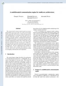
Fig. 3.2: Operators in mirrored tree view Work share distribution. In order to design efficient parallelization models it is indispensable to understand the distribution of the computational work among the operators at all levels of the tree. We analyze the breakdown of such based on an example with N = 20 · 106 particles uniformly distributed in the unit cube, an octree of height h = 7 and give results for an accuracy Acc = 7 (for the definition of Acc see the remark at the end of Sec. 2.1). Recall, the accuracy 6
does only influence the work share of the far-field computation (see Sec. 2.1). The work share of the near-field computation is not affected as long as the height of the tree coincides. Here, it is 0.78 TFlop (28.75 %) versus 2.71 TFlop (71.25 %) for the far-field, whose computational cost increases with respect to the accuracy. In Fig. 3.3 we study the percentage share of the overall number of required floating point operations for level-wise grouped operators (far-field: P2M, M2M, M2L, L2L, L2P and near-field: P2P). The directed edges indicate the dependencies between the operators. The far-field computation starts with the P2M at level 6 (the leaf level), once it is concluded the M2L at the leaf level and the M2M at level 5 are ready, and so on. The work share of the M2L is clearly predominant. Moreover, as we climb down the tree the work share, hence also the parallelism, increases. In fact, most of the work is done by the operators at the leaf level. The reason is that the number of cells between parent and child level behaves like 1/8 (because of the uniform particle distribution). Another important aspect is the work share between near-field and far-field. For the same example as above, but with Acc = 3 (instead of Acc = 7), the ratio between far-field and near-field changes from 28.75 % vs. 71.25 % to 4.50 % vs. 95.50 % (removing one level of the octree would yield a similar ratio). Examples with a large near-field and a small far-field work share are easier to parallelize than vice versa. For an efficient Far-field M2M 0.0002%
M2L 0.0042%
L2L 0.0002%
M2M 0.002%
M2L 0.070%
L2L 0.002%
M2M 0.016%
M2L 0.750%
L2L 0.016%
M2M 0.13%
M2L 6.88%
L2L 0.13%
P2M 0.89%
M2L 58.75%
L2P 3.60%
Near-field
P2P 28.75%
Fig. 3.3: The breakdown of the computational work (N = 20 · 106 and h = 7 and Acc = 7) shows dependencies between the FMM operators at different levels and their percentage share of the overall work (total work 2.71 · 1012 Flop with 71.25% far-field and 28.75% near-field). design of parallelization models of the FMM some aspects need to be taken into account. Let us recap them. • The near-field and far-field computations are (nearly) independent. • The far-field provides much parallelism at the bottom and little towards the top of the tree. • The near-field is easy to parallelize, the far-field is not. In the remainder of this section we exploit these aspects in a step-by-step fashion to obtain a highly efficient parallelization of the FMM algorithm. 3.1. Fork-join model. Naive Fork-join model. The most straightforward way of parallelizing the FMM is to force the algorithm to progress level by level and split the work at each level between the threads. Algorithm 1 shows such a level-wise progression. The high-level algorithm (function FMM in 7
Alg. 1) simply consists of a sequence of calls to the FMM operators at the different levels of the tree, without exhibiting any reference to an OpenMP statement. The parallelization is indeed only performed within the operators (shown for instance for the M2L operator - function M2L - in Alg. 1) using the simple and popular omp parallel for statement [13]. This statement performs an implicit barrier (all threads are joined) at the end of the loop to which it is applied, it is immediate to observe that the correctness of the execution is guaranteed. However, forcing three barriers at each level may induce a non negligible performance penalty. In the sequel, we refer to this scheme as the naive fork-join model. Algorithm 1: Naive Fork-join model for the FMM algorithm function FMM(tree, kernel) // Near-field P2P(tree.levels[tree.height-1]); // Far-field P2M(tree.levels[tree.height-1]); for l = tree.height-2 ! 2 do M2M(tree.levels[l]); for l = 2 ! tree.height-2 do M2L(tree.levels[l]); L2L(tree.levels[l]); M2L(tree.levels[tree.height-1]); L2P(tree.levels[tree.height-1]); // M2L implementation example function M2L(level) #pragma omp parallel for foreach cell cl in level.cells do M2L(cl.local, cl.far_field.multipole); // Implicit barrier from omp parallel
Fork-join model. Synchronization points may be alleviated in different manners. Although more complicated OpenMP codes are possible, we chose the following sequence of steps in order to improve the performance: perform all M2Ms (with a synchronization point between levels required by the algorithm), then all P2Ps and M2Ls (which provides the maximum concurrency and opportunities for load-balancing), and finally the L2Ls and L2Ps. The DAG does not require to complete all M2Ms before starting the M2Ls. However taking advantage of that property of the DAG, while avoiding the lack of concurrency at the top of the tree, requires a complex scheduling that concurrently executes the M2M with the M2L. We considered such optimization beyond the scope of a “reasonably simple” OpenMP algorithm. From experiments, we found that it is better to compute the P2P before the M2L because in many cases the P2P can be more nonuniform. Such algorithm is detailed in Alg. 2. There are now only two barriers per working level. Granularity. Up to now, each operator call operates only on a single cell. For example in the simple fork-join model, a P2P call evaluates the at most 26 near-field interactions of one cell at the leaf level. Or an M2M call computes the equivalent source values based on the source values 8
Algorithm 2: Fork-join model for the FMM algorithm function FMM(tree, kernel) #pragma omp parallel // Far-field Upward pass P2M(tree.levels[tree.height-1]); for l = tree.height-2 ! 2 do M2M(tree.levels[l]); // Near-field P2P_nowait(tree.levels[tree.height-1]); // Far-field Transfer pass for l = 2 ! tree.height-1 do M2L_nowait(tree.levels[l]); // Wait M2L and P2P to finish #pragma omp barrier; // Far-field Downward pass for l = 2 ! tree.height-2 do L2L(tree.levels[l]); L2P(tree.levels[tree.height-1]); // M2L implementation example function M2L_nowait(level) #pragma omp for nowait schedule(dynamic, Chunk_size) foreach cell cl in level.cells do M2L(cl.local, cl.far_field.multipole); // No barrier
of its 8 child cells and an M2L call computes at most 189 far-field interactions. This model has a negative impact on the overall performance due to the following aspects: • Large number of operator calls: there are at most 8l cells at level l, hence, the same number of operator calls. • Large number of dependencies: a cell has at most 189 far-field interactions and a leaf cell has at most 26 near-field interactions which must be made available to each operator call; • Small granularity of far-field operators: depends on number of particles in leaf cells and the accuracy Acc. In order to remedy these issues we introduce a parametrization of the granularity of these operator calls. The idea is presented in Fig. 3.4 and we refer to it hereafter as the blocked fork-join model. Instead of a tree where nodes represent cells (left figure) we move to a tree where nodes represent blocks of at most ng cells (right figure) and let each operator call operate on such a block of cells. Note that in the trivial case with ng = 1 the blocked fork-join model reduces to the simple one. We use the Morton ordering [14] for indexing cells within the octree and, hence, also for the assembly of blocks of cells. That is, why they tend to be grouped also locally and, hence, they very likely share common near and far-field interactions. Because of this increased data locality operator calls of larger granularity lead to a higher performance in their execution. However, as result of coarser granularity we get fewer operator calls which limits the concurrency. It is 9
Fig. 3.4: A tree with ng = 3 (one node in the tree groups three cells)
essential to find values for ng the granularity to find the optimal trade-off between performance and concurrency. In Alg. 3 we use parametrized operator calls with the omp parallel for statement exemplary for the near-field computation. It works analogously for the far-field and we can plug such into Alg. 2 in order to obtain a blocked fork-join model for the FMM algorithm. We do still have a barrier at each level. Algorithm 3: Blocked fork-join model for the P2P operator function P2P_nowait(level) #pragma omp for nowait foreach block of cells bl in level.blocks do P2P(bl.particles, bl.near_field.particles);
3.2. Interleaving near-field and far-field computations. In the previous models we studied sequential executions of parallel regions which is the usual way of parallelizing the FMM. We did not exploit the fact that the near-field and far-field computations are (nearly) independent. Here, we present a model that exploits this property by replacing the loop parallelization by a task parallelization strategy (see Alg. 4). We use the omp task model. In the following we describe why that allows us to interleave the computations of near and far field. We use the omp sections statement for splitting the FMM algorithm in two: the first section is concerned with the near-field computation and the second section with the far-field computation. All created threads enter the omp sections scope but only two move on to the two omp section scopes (one each). The remaining threads wait at the end of the omp sections scope. For the computation of near- and far-field we use the omp task statement (see Alg. 5 for the M2Ltask implementation). Now, the two active threads create tasks, deliver them to the OpenMP runtime which schedules them to the waiting threads which execute them concurrently. The omp taskwait barriers in the far-field section (see Alg. 5) can be partially hidden by the concurrent task insertion in the near-field section: imagine, there are not enough far-field task available due to a taskwait barrier, threads, instead of being idle till the end of that barrier, can proceed with available near-field tasks. Recall, that the near-field and far-field computation is only nearly independent, because both, P2P and L2P write indeed on the same values (see Sec. 2.1). We implement this reduction manually by introducing an omp single directive before calling the L2P in Alg. 4. Note that in Alg. 5, M2L tasks operate on blocks of cells and not on single cell. The reason is the following. Assume, ts is the time needed by the runtime system to create/schedule/destroy a task, te is the time to execute a task and nt the number of available threads. As long as nt ts > te 10
Algorithm 4: Interleaving near-field and the far-field computations function FMMtask(tree) #pragma omp parallel #pragma omp sections // Near-field #pragma omp section P2Ptask(tree.levels[tree.height-1]); // Far-field without L2P #pragma omp section P2Mtask(tree.levels[tree.height-1]); for l = tree.height-2 ! 2 do M2Mtask(tree.levels[l]); for l = 2 ! tree.height-1 do M2Ltask_notaskwait(tree.levels[l]); // Wait for M2L tasks to finish #pragma omp taskwait; for l = 2 ! tree.height-2 do L2Ltask(tree.levels[l]); // Reduction with L2P #pragma omp single L2Ptask(tree.levels[tree.height-1]);
Algorithm 5: Task model for the M2L and M2M operators function M2Ltask_notaskwait(level) foreach block of cells bl in level.blocks do #pragma omp task M2L(bl.local, bl.far_field.multipole); function M2Mtask(level) foreach block of cells bl in level.blocks do #pragma omp task M2M(bl.multipole, bl.children.multipole); #pragma omp taskwait;
is true, not sufficient work will be available for all threads. By increasing the granularity of tasks we increase te and as a consequence the overhead for the runtime system to handle the tasks becomes negligible. Preliminary studies (not reported here) have shown that Alg. 4 with tasks of too fine granularity does not scale. According to our knowledge of the OpenMP standard, this algorithm is the one of the most efficient, in terms of pipelining, which can be obtained using simple OpenMP statements. In fact, OpenMP does not provide a feature which allows to express dependencies between tasks or to give priorities to them even if such system can be developped by hand. 11
3.3. Task flow. At the beginning of Sec. 3 we created a directed acyclic graph (DAG, see Fig. 3.2) to express the dependencies between tasks which are represented by its nodes. In the following we turn that DAG into one where nodes represent tasks and edges carry the dependencies (see Fig. 3.5). This is the natural representation for runtime systems like StarPU M2L M2L
P2M M2L P2M
P2M
M2M
M2M
M2L
L2L
L2L
P2M
L2P
P2P
L2P
P2P
L2P
P2P
L2P
P2P
M2L M2L
Fig. 3.5: The task flow of the FMM algorithm given by a DAG where nodes represent tasks and edges dependencies (straight lines represent a writing operation from different tasks on the same memory). (Sec. 2.2), which model them internally. To create the dependencies, StarPU uses the order of insertion of the tasks and the kind of access mode they apply to the data. In StarPU the insertion of tasks is performed asynchronously in other words the computation and the tasks insertion are done in parallel. The main thread calls a method to insert a task into the runtime system which has a prototype like insertTasks(codelet, access_mode_1, handle_1, access_mode_2, handle_2, ...); The access modes can either be READ, WRITE or READ_WRITE. They express the access mode of data handles which are a key structure to enable the data management in StarPU. Data handles with READ access mode can be processed simultaneously. However, in order to obtain correct and defined results, data handles with WRITE access mode have to be processed one after another. Based on this concept the entire DAG and, thus, the insertion order of all tasks is defined. 3.3.1. Refining the task flow. Generally, when processing the DAG the following two aspects have to be considered. 1) A strict execution order requires one task to be processed after the other one. For example, one task depends on the result of the previous one. 2) A flexible execution order prohibits a simultaneous execution of tasks but does not prescribe which to process first. For instance, if two tasks want to write on the same memory simultaneously a race condition arises and no statement about the correctness of the result can be made. In the FMM DAG both types of execution orders occur. Strict ones are met for M2M tasks. Before processing the M2M tasks at level l those from level l 1 have to be completed. Flexible ones are met for L2L and M2L tasks. At a given level l it does not matter which of the two tasks is processed first. The same situation is met for P2P and L2P tasks. Both are writing on the same data. They add the near-, respectively far-field contribution to the target values (see Sec. 2.1). In the following we will show how the flexible execution order allows to refine and optimize the task flow. L2P before/after P2P. P2P tasks are independent from all other tasks except L2P tasks which come at the end of the far-field computation. As we mentioned above, in order to satisfy dependencies between them it does not matter which one we process first. We first insert L2P 12
and then P2P tasks. This puts P2P tasks at the very end of the task flow as shown in Fig. 3.6a and StarPU allows P2P tasks to be executed only once all L2P tasks are completed. Our objective is, however, to use P2P tasks to remedy concurrency bottlenecks during the far-fields computation. We can do so by inserting P2P before L2P tasks (see Alg. 6). Now L2P tasks start being executed once all other far-field and P2P tasks are completed. But P2P tasks are available all the time. The resulting task flow is presented in Fig. 3.6b. Algorithm 6: P2P before L2P foreach block of cells bl in leaflevel.blocks do insertTask(P2P, READ_WRITE, bl.particles, READ, bl.near_field.particles); foreach block of cells bl in leaflevel.blocks do insertTask(L2P, READ_WRITE, bl.particles, READ, bl.local);
In Fig. 3.6 we can see that inserting P2P before L2P tasks leads to a task flow with more tasks without predecessors which are available right away, thus, it provides more parallelism. Note, M2L
M2L
M2L
M2L
P2P L2P
P2M M2L P2M
M2M
L2L
M2M
L2L
L2P
P2P
P2M
L2P
P2P
P2M
L2P
P2P
P2M
L2P
P2P
P2M
L2L
L2P
M2L M2M
P2P P2P
P2M
M2L
P2M
M2M
M2L
M2L
M2L
M2L
M2L
(a) L2P before P2P
L2P L2L L2P
P2P
(b) P2P before L2P
Fig. 3.6: DAG generated by the two P2P and L2P tasks insertion algorithms. both, P2P and L2P tasks have READ_WRITE access on bl.particles, because both increment their target values f . This is the reduction after the independent execution of near- and far-field. M2L before/after L2L. The execution order of M2L and L2L tasks is important as it might induce barriers during the computation. L2L tasks at level l have READ access to cells at level l and READ_WRITE access to their child cells at level l + 1. M2L tasks at level l have READ and WRITE access on cells at level l. Hence, both, L2L tasks at level l 1 and M2L tasks at level l have WRITE access on cells of level l. Meaning that these tasks cannot be executed simultaneously but the order of their execution does not matter. There are two situations for far-field tasks to satisfy dependencies. First, M2M tasks at level l + 1 have to be completed before M2L tasks at level l can be executed. Secondly, M2L tasks at level l and L2L tasks l 1 have to be completed before L2L tasks at level l can be processed. We can choose to execute L2L tasks at level l 1 before we execute M2L tasks at level l. This choice is presented in Alg. 7 and the resulting task flow can be seen in Fig. 3.7a. It delays 13
the insertion of the M2L tasks of the leaf level which provide the most parallelism. The reason is that first the L2L tasks from the level above the leaf level have to be completed which means that all M2M and L2L and all M2L except the one from the leaf level have to be completed, too. Algorithm 7: L2L before M2L for l = tree.height-2 ! 2 do foreach block of cells bl in tree.levels[l].blocks do insertTask(M2M, WRITE, bl.multipole, READ, bl.children.multipole); for l = 2 ! tree.height-2 do foreach block of cells bl in tree.levels[l].blocks do insertTask(M2L, READ_WRITE, bl.local, READ, bl.far_field.multipole); foreach block of cells bl in tree.levels[l].blocks do insertTask(L2L, READ_WRITE, bl.children.local, READ, bl.local); foreach block of cells bl in tree.levels[tree.height-1].blocks do insertTask(M2L, READ_WRITE, bl.local, READ, bl.far_field.multipole);
The second choice is to execute first M2L tasks at level l and then L2L tasks at level l 1 and is presented in Alg. 8. In the resulting task flow in Fig. 3.7b can be seen that M2L tasks at level l become available just after M2M tasks at level l + 1 are concluded. In theory such order of execution might create a small lack of parallelism if all M2L tasks are concluded but L2L tasks not. However, in practice, the cost of L2L compared to M2L tasks is negligible. This approach releases quickly much parallelism and it is to choose over the previous one. Algorithm 8: M2L before L2L for l = tree.height-2 ! 2 do foreach block of cells bl in tree.levels[l].blocks do insertTask(m2m, WRITE, bl.multipole, READ, bl.children.multipole); foreach block of cells bl in tree.levels[2].blocks do insertTask(m2l, READ_WRITE, bl.local, READ, bl.far_field.multipole); for l = 2 ! tree.height-2 do foreach block of cells bl in tree.levels[l+1].blocks do insertTask(m2l, READ_WRITE, bl.local, READ, bl.far_field.multipole); foreach block of cells bl in tree.levels[l].blocks do insertTask(l2l, READ_WRITE, bl.children.local, READ, bl.local);
3.3.2. Scheduling strategies. Since the computation is split in tasks, it remains important to organize the order of execution of tasks among available processing units. This is done by the scheduler. Its choices and capabilities have a big impact on the performance of the parallel execution. Each task has a state which can be either blocked or ready. Blocked tasks need to wait until those it depends on are finished. Whereas, ready tasks have all their dependencies satisfied and can be executed right away. The scheduler is the system in charge of ready tasks, only. It manages their order of execution and their assignment to available processing units. The idea 14
P2P L2P
M2L
M2L
P2P
M2L L2P
M2L P2M M2L P2M
L2P
L2L
P2M
M2M
P2P
P2P P2M
M2M
P2P
L2P M2L
L2P
M2L
P2P
M2M
L2L
P2M
P2M
L2L
P2M
M2M
M2L
M2L
L2P L2L
P2M
L2P
M2L
M2L
M2L
L2P
P2P
(b) M2L before L2L
P2P
(a) L2L before M2L
Fig. 3.7: DAG generated by the tasks insertion of algorithm 6 followed by 7 or 8
is the following. Each scheduler owns one or more containers (list, queue, FIFO, etc.) which store ready tasks. The runtime system passes ready tasks to the scheduler by calling push. At the same time, pop releases tasks to available processing units (also workers). The scheduler specific implementation of these two methods push and pop is visible in the Figs. 3.8 and 3.9. Any scheduler in StarPU has to implement these two methods and is obligated to make sure that all tasks given to be schedule are also released, i.e. the containers are emptied. The number of ready tasks can be high, and scheduling has to be efficient, i.e., the time for scheduling a task must be negligible compared to the time required for it execution. Moreover, the scheduler needs to be able to deal with heterogeneous processing units, various kinds of tasks and potential data transfer between different processing units. Some scheduler allow the user to give hints to fill processing units and to make it doing correct choices. The scheduling strategy in such context is an ongoing research topic. Along with StarPU come several scheduler. One of them is the Eager scheduler which we compare with the Priority scheduler, which we developed specifically for the FMM algorithm. In the following we first briefly introduce the Eager scheduler and then in more details the Priority scheduler. Finally, we compare both schedulers. Eager scheduler. The Eager scheduler is described in StarPU [1]. Its behavior is based on the greedy algorithm. push consists in storing the newly ready tasks in a single container. When a worker calls pop Eager releases the head of the container. Such scheduling is very cheap since it reduces the scheduling time to a minimum, no choice needs to be made. On the other hand, there is no distinction between tasks and bad choices might be taken. For example, it does not allow the user to have any influence on the scheduling (as opposed to the Priority scheduler which we introduce later). In Fig. 3.8 we outline the mechanics of this scheduler. Priority scheduler. In the following, we present the MultiPrio scheduler we developed and show its efficiency to pipeline FMM tasks. To be able to control the task flow, we developed a scheduler that supports the assignment of priorities to tasks. These priorities lie in the range from 0 to MAX_PRIO: 0 denotes the highest and MAX_PRIO the lowest priority. The choice of the priority for a task may depend on its type and on the level in the octree it operates on. Such 15
User
StarPU Core
Eager (Scheduler)
Workers (PU) P
?
X
X
X
R
Insert a new task
R
Push ready task
C P U
Pop task
Task legend: ? : Unknown status X : Not ready R : Ready P : Currently processed F : Finished
C P U
F
Release dependencies
Fig. 3.8: The Eager scheduler
flexibility of assigning different priorities to different types of tasks lead to a much better pipeline of the task flow. In Fig. 3.9, we present the structure of the MultiPrio scheduler. As opposed User
StarPU Core
MultiPrio 2
R 0
?
2
0
X
Insert a new task
X
Workers (PU)
2
R
2
R
P
1
X
C P U
1
R
Push ready task
Pop task 0
R
C P U
F
Task legend: ? : Unknown status X : Not ready R : Ready P : Currently processed F : Finished
0
R
Priority
Release dependencies
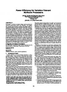
Fig. 3.9: Priority scheduler to the Eager scheduler, it has several containers to store tasks of a given priority each. With push, we add tasks which are ready to the container for the relative priority. Then, with pop we iterate through the containers storing the tasks and release those with the highest priority first and those with the lowest priority last. 4. Numerical Studies. In the previous section, we have presented how the FMM algorithm can be turned into a task flow which, as a consequence, can be executed by a runtime system. We constructed this scheme in a step-wise fashion. We started with the well known simple forkjoin parallelization model of the FMM. We introduced a blocking of cells in order to increase the granularity. We interleaved near- and far-field computations by using the task model from OpenMP and finally we presented the full task flow model. In this section we compare and validate all these models. We start by presenting the two examples we use for that and two homogeneous machines we use for the computations. Then we study various settings and identify the most efficient ones. Finally we study the parallel efficiency and compare the presented parallelization models in detail. In the whole study, we only assess the numerical step and we thus do not take into account the preliminary symbolic step (essentially consisting of the octree setting). 4.1. Experimental setup. We consider two different example geometries with different types of particle distribution, respectively. Cube (volume) Corresponds to random sampling particles in the unit cube as illustrated in Fig. 4.1a. Such distributions have approximately the same number of particles per leaf 16
cell. Also each cell has all its neighbors. Ellipsoid (surface) Corresponds to a sampling of particles on a the surface of the ellipsoid with a higher density at the extremities as illustrated in Fig. 4.1b. Such distributions lead to octrees where the ratio of the leaf cell with the most particles versus the one with the least particles might be 1. Also, an adaptive structure for the octree, introduced in section 2.1, needs to be used in order to achieve good performance .
(b) Ellipsoid (surface)
(a) Cube (volume)
Fig. 4.1: Particles distributions of the test cases. We consider two different homogeneous platforms for assessing our algorithms for the above examples. 4 deca-core Intel Xeon E7-4870 This platform is composed of four deca-core Intel Xeon E74870 processors running at 2.40 GHz (40 cores total). This machine is cache-coherent with Non Uniform Memory Access (ccNUMA), which means that each core can access the memory available on all sockets, with a higher latency if the accessed data is on another socket. Each socket has 256 MB of random access memory (RAM) and a 30 MB L3 cache. Each CPU core has its own L1 and L2 caches of size 32 KB and 256 KB, respectively. 20 octa-core Intel Xeon E7-8837 This machine is an SGI Altix UV 100. It is also a ccNUMA machine, composed of twenty octa-core Intel Xeon E7-8837 processors running at 2.67 GHz (160 cores total). Each socket has 32 GB of RAM and 24 MB of L3 cache. Each CPU core has its own L1 and L2 caches of size 32 KB and 256 KB, respectively. We use the Intel compiler (version 12.0.5.220) with the compilation flags -ip -O2. We have assessed different NUMA policies for the memory allocation. In the present study, we use a memory interleave policy as it achieved the highest performance. Memory is allocated using round robin on all memory nodes with the “numactl –interleave=all” option. We have also tuned the OpenMP environment. We have binded the threads to the CPU cores by setting the “OMP_PROC_BIND=true” environment variable and we have enabled an active waiting policy by setting the “OMP_WAIT_POLICY=ACTIVE” variable. The OpenMP codes rely on the Intel OpenMP Runtime Library embedded with the compiler. The task flow codes rely on 17
StarPU 1.0.0rc3. To assess the parallel efficiency, we present traces of execution of FMM computation. The color legend for the tasks is illustrated in Fig. 4.2, red (dark) stands for idle time, white stands for P2P tasks, light-gray for M2L tasks and gray tasks for all other tasks (P2M, M2M, L2L and L2P).
idle
P2P
M2L
other kernels
Fig. 4.2: Color legend for traces
4.2. Refining the settings. In order to come up with the optimal settings of our method here we perform numerical studies on the block size and we compare both presented schedulers. Based on these studies we choose the settings which lead to the most efficient computations in terms of pipelining the task flow and computational times. Block size. Obviously the optimal block size ng depends on the example and the machine we use for the computation. Too small values lead to too many tasks of too small granularity. Too large values lead to too few tasks and, hence, not all threads may have work. Our goal here is to find out if there exists a range of values for ng which lead to efficient computations independent of example and machine. In Fig. 4.3 we plot the achieved performance of different examples computed on both machines for a large range of ng . Interesting is the benchmark for the cube (volume) with N = 20 · 106 particles on the 20 octa-core Intel Xeon E7-8837. It is best performing for 250 < ng < 1 000. This is a rather small interval compared to the other benchmarks. The reason is that larger ng do not provide enough parallelism anymore. For N = 20 · 106 particles and h = 7 there are 86 = 262 144 cells at the leaf level. With 160 threads the block size cannot exceed ng < 86 /160 ⇠ 1 638 otherwise there will not be work for each thread. Particle distributions on surfaces, e.g., the ellipsoid (surface), represent the trickier case. The set of far-field interactions for the cube (volume) is complete, i.e. each cell has 63 33 = 189 cells in its far-field. This is not the case for the ellipsoid (surface), indeed it behaves more like 62 32 = 27. Moreover, the number of far-field interactions can change considerably. Thus, for particle distributions on a surface tasks of block size ng provide less work than it is the case for particle distributions in the volume. Moreover, if we fix the number of particles N and their bounding box the particle density is much higher in the case of a particle distribution on a surface. Thus, a higher octree needs to be constructed which leads to many more cells (in fact their number 8h for volume and 4h for surface distributions grows exponentially in h). Another issue in the case of a particle distribution on a surface is that the ratio of the leaf cell containing the most particles to the one containing the least particles may be 1. Hence, if we solely use ng to define the granularity of a task we actually end up having tasks (P2M, L2P and P2P) with vastly different numbers of particles. If we look at the studies for the 4 deca-core Intel Xeon E7-4870 machine in Fig. 4.3 we note that the achieved performance is almost the same for any ng in the studied interval, except for very small values ng < 500. This tells us that the N = 20 · 106 particles example provides enough parallelism on that machine, and that is why we do not study larger examples on it (see Tab. 4.1). This is different on the 20 octa-core Intel Xeon E7-8837 machine. The examples with N = 20·106 perform well for ng 2 [500, 2 500] for the cube (volume) and ng 2 [1 500, 5 500] for the ellipse (surface). Then the achieved performance breaks down and approaches the one obtained on the 4 deca-core Intel Xeon E7-4870 machine. We can indeed observe that for large block 18
sizes (ng = 10, 000 for the 20.106 particles cube, ng = 18, 000 for the 20.106 particles ellipsoid), using 160 CPU cores does not bring more performance than using 40 CPU cores. Of course, in practice, we select a much smaller block size to benefit from all 160 CPU cores (ng = 750 for the cube, ng = 3000 for the ellipsoid, see Fig. 4.4). The large examples, with 200 · 106 and 100 · 106 particles for cube (volume), respectively ellipsoid (surface) show a similar invariance on ng as seen for the smaller examples on the 4 deca-core Intel Xeon E7-4870 machine. In the remaining sections, the block size is tuned for the 4deca, cube, N = 20 · 106
4deca, ellipse, N = 20 · 106
20octa, cube, N = 20 · 106
20octa, ellipse, N = 20 · 106
20octa, cube, N = 200 · 106
20octa, ellipse, N = 100 · 106
Performance (GFlop/s)
300
200
100
0
0
0.2
0.4
0.6
0.8
1
1.2
1.4
1.6
Block size ng
1.8
2
·104
Fig. 4.3: Parallel performance on the 4 deca-core Intel Xeon E7-4870 (4deca) and 20 octa-core Intel Xeon E7-8837 (20octa) machines for different block sizes ng 2 (0, 20000]. Presented are studies for the cube (volume) (N = 20 · 106 with h = 7 and N = 200 · 106 with h = 8) and the ellipse (surface) (N = 20 · 106 with h = 10 and N = 100 · 106 with h = 12). The chosen accuracy is Acc = 5. number of particles, the type of distribution (cube or ellipsoid), the tree height and the target machine. This tuning step is performed empirically, by selecting the fastest execution among multiple block sizes. Presenting all the selected block sizes being unusefully verbose, we only provide typical block sizes that were selected by this process in Tab. 4.1. Note that this selection process is conducted for each parallelization scheme.
Machine 4 deca-core Intel Xeon E7-4870 20 octa-core Intel Xeon E7-8837
Cube (volume) small large 1 500 1 000
not studied 3 000
Ellipsoid (surface) small large 6 000 3 550
not studied 8 000
Table 4.1: Typically chosen block sizes ng . (On the 4 deca-core Intel Xeon E7-4870 machine, large examples are trivial to parallelize and, thus, not interesting to study.)
19
Ellipsoid (surface) h = 10, ng = 3000
Cube (volume) h = 7, ng = 750
Tree height. As discussed above, the execution time strongly depends on the octree height h. However, preliminary experiments (not reported here) have shown that the optimum octree height h is not very sensitive to the number of CPU cores employed. Therefore, the octree height is chosen such that the sequential computational time is minimized and we use the same height tree for parallel executions. In particular, the same height tree is used for all parallelization schemes for a given particle distribution and accuracy. This process almost consistently led to an optimum height tree for all parallel schemes. Scheduler comparison. In Fig. 4.4 we compare traces of simulations obtained via the Eager and the Priority scheduler. Each line in the traces stands for one thread over time. In the case of the cube (volume) example both traces look almost the same, both, in terms of time and tasks execution. Scheduling in that case is easy. The main difference is when P2P tasks are Eager scheduler
Priority scheduler
(a) t = 15.9 s
(b) t = 15.9 s
(c) t = 7.9 s
(d) t = 6.9 s
Fig. 4.4: Comparison of traces obtained from the Eager and the Priority scheduler for the cube (volume) and ellipsoid (surface) with N = 20·106 on the 4 deca-core Intel Xeon E7-4870 machine. The granularity of the tasks is parametrized by ng . executed. Eager inserts them at the same time as it inserts M2L tasks. By means of the Priority 20
scheduler we are able to give M2L and P2P tasks different priority. In the case of the particle distribution in a volume this is not yet apparent. As we have already explained above, particle distributions on a surface, such as the ellipsoid (surface) leads to max{Nleaf }/ min{Nleaf } 1 where Nleaf denotes the number of particles per leaf cell. Note, that the cost of the P2M and 2 L2P grows like O(Nleaf ), but the one for the P2P task grows like O(Nleaf ). Consequently, we decided to differentiate between P2P(large) and P2P(small) tasks and to assign them different priorities within the Priority scheduler. The Eager scheduler does not allow that and we can see in Fig. 4.4c the negative impact in the trace. Some of the P2P(large) tasks are executed before the M2L tasks and the remaining ones after. At that stage of the execution no other tasks are available which could give work to the idle threads. Within the Priority scheduler we assign the P2P(large) tasks a higher and the P2P(small) a smaller priority with respect to the M2L tasks. That is why the ponderous P2P(large) tasks are executed right away and the sleek P2P(small) tasks are used after the M2L tasks in order to give idle threads work. The resulting trace is presented in Fig. 4.4d. We do also give individual priorities to all other tasks as can be seen in Tab. 4.2. As we identify 7 different types of tasks we consider a maximum of 7 + 2h priorities priority index
type of task
priorities
1 2 3 4 5 6 7
P2M M2M L2L(l) P2P(large) M2L(l) P2P(small) L2P
0 1 l 2 [2, h 2] h 1 h + l 2 with l 2 [2, h 2h 2 2h 1
1]
Table 4.2: Assigned priorities (l denotes the level in the octree the respective L2L(l) or M2L(l) tasks operates on). Note that all priorities of tasks at index i + 1 have to be strictly larger than those at index i; h is the oct-tree height. (h is the octree height). In fact, five types of tasks (P2P(small) and P2P(large), P2M, M2M and L2P) are assigned static priorities and two types of tasks (M2L(l) and L2L(l)) are assigned priorities which depend on the respective level l in the octree they operate on. The priorities decrease as h decreases. 4.3. Comparison of all parallelization models. In Sec. 3.3 we have presented a total of four different parallelizations models for the FMM algorithm. For the sake of simplicity we introduce abbreviations for them. • SFJ stands for simple fork join model and is presented in Sec. 3.1. • BFJ stands for blocked fork join model and is also presented in Sec. 3.1. • INF stands for interleaving near- and far-field and is presented in Sec. 3.2. • TFL stands for task flow model and is presented in Sec. 3.3. In Fig. 4.5, we study how the performance, measured in GFlop/s, of these four models evolves as we increase the number of particles N in the cube (volume) and on the ellipsoid (surface). Since the octree height h is chosen such that the computational time is minimized (see Section 4.2), h naturally increases with N . For example, in Fig. 4.5a, a height h = 7 was seleced for 107 N < 5 · 107 and h = 8 for N 5.0 · 107 . Also, in the studies we confront the theoretical upper bound and the actual parallel performance. The theoretical upper bound is given by the sequential performance multiplied by 160, i.e. the number of cores on the 20 octa-core Intel Xeon E7-8837 21
machine. The BFJ, INF and TFL models have similar theoretical upper bounds. The SFJ model looses, it is the only model which does not exploit data locality due the blocking of cells. Let us focus on the intervals of N for h = 8 and of N for h = 12 in Fig. 4.5a, and Fig. 4.5b which show the performance behavior. The octree height is constant, hence the work spent for the far-field computation is the same for the entire interval and only the work spent for the near-field computation grows with N . As the P2P tasks are mutually independent, the near-field computation is trivial to parallelize. That is why the problems with N being at the upper range (where the near-field is strongly dominant) are easy to parallelize and any parallelization scheme shall reach a performance close to the theoretical upper bound. On the other hand, when N is close to the lower range of the interval, the far-field is predominant which makes the FMM hard to parallelize. The reason for the higher upper bound in the lower range of N is that the far-field operators (mainly M2L) achieve a much higher sequential performance (3.8GFlop/s) than the P2P operator (2GFlop/s). We now focus on the parallel performance of all four models. First, for the cube (volume), all models are roughly equivalent. The SFJ is paying the price of the non-block data structure and is slower. Three other models, BFJ, INF and TFL are very close. We remind that in the cube (volume) with a uniform data distribution, 95% of the work is composed of the P 2P and the M 2L at the last level of the tree. The data are stored in block and therefore the computational time for each block is almost the same. Then, the parallelization is very easy and no bad choice can be made. It is also interesting to notice that StarPU is achieving the same performance even if it pays an extra cost to manage each block of data and task dependencies. The performance of all four models tends to approach the asymptote for the theoretical upper bound. We claim that the TFL model is better than the other on the ellipsoid (surface) example presented in Fig. 4.5b. This type of example is harder to parallelize than the cube (volume) case, because it leads to non uniformly sized tasks. In fact, the octree is non uniform and the ratio of the biggest (containing the most particles) leaf cell over the smallest leaf cell can be large. Despite this problem, the TFL model is the only model which reaches a parallel performance of about 71 % of the theoretical upper bound. Also the INF model, which is the second best one, reaches 64 % of the parallel performance. The SFJ and the BFJ models reach only 35 % and 30 % of their respective theoretical upper bound of the parallel efficiency. However, for a small number of particles and it seems that the cost of using StarPU is non negligible. Furthermore, we give some execution timing to show how difficult it is to parallelize simulations with a small number of particles. If we consider the execution of the ellipsoid (surface) with N = 20 · 106 and h = 11, the execution time for TFL model is 234 s in sequential, and 2.05 s in parallel for the same model. If we consider the execution of the cube (volume) with N = 10 · 106 and h = 7, the execution time for TFL model is 211 s in sequential, and 1.99 s in parallel for the same model. Remark It is not entirely true that for a constant octree height h but increasing number of particles N only the cost of the near-field grows and the cost of the far-field remains constant. The reason is that also the far-field operators P2M and L2P involve particles. However their cost growth is negligible because of two reasons. Their cost compared to the one of the M2L operator is vanishingly small (recall Fig. 3.3) and the cost per P2P grows quadratically with Nleaf and the cost per P2M and L2P only linearly. 4.4. Parallel efficiency of the task flow model. Above we have compared the performance of the four models and as a result we identified the TFL to be the clear winner. We now study the parallel efficiency en , defined as en =
t1 , ntn
22
Performance
GFlop/s
500
400
300
200
100
0
h=5
SFJ in sequential times 160
SFJ 160 CPUs
BFJ in sequential times 160
BFJ 160 CPUs
INF in sequential times 160
INF 160 CPUs
TFL in sequential times 160
TFL 160 CPUs
h=6
105
h=7
106
107
h=8 108
Number of Particles
(a) Cube (volume)
Performance
GFlop/s
500
400
300
200
100
0
h=7 105
h=8
h=9
h = 10
106
h = 11 107
h = 12 108
Number of Particles
(b) Ellipsoid (surface)
Fig. 4.5: Performance GFlop/s of all four parallelization models on the 20 octa-core Intel Xeon E7-8837 machine for varying N and h and a fixed accuracy Acc = 5. The sequential performance multiplied by 160 (the number of threads) gives the upper bound for the respective model. SFJ: simple fork-join, BFJ: block fork-join, INF: interleaved near and far field, TFL: StarPU.
23
for this model. In the above equation tn denotes the wall time needed for n computational units (e.g., CPU cores in our case). In the Figs. 4.6 and 4.7 we present studies obtained on the 4 deca-core Intel Xeon E7-4870 and the 20 octa-core Intel Xeon E7-8837 machine, respectively, for different N in the cube (volume) and on the ellipsoid (surface) and for the accuracies Acc = 3, 7.
Parallel efficiency en
1 0.8 0.6 0.4
Acc = 7, cube (volume) Acc = 3, cube (volume)
0.2
Acc = 7, ellipsoid (surface) Acc = 3, ellipsoid (surface)
0
0
5
10
15
20
25
30
35
40
Number of CPUs
Fig. 4.6: Parallel efficiency en on the 4 deca-core Intel Xeon E7-4870 machine for N = 20 · 106 particles in the cube (volume) with h = 7 and ng = 1500 and on the ellipsoid (surface) with h = 11 and ng = 6000.
All studies show strong scaling. On the 4 deca-core Intel Xeon E7-4870 machine we obtain up to 91 % efficiency for all four examples (see Fig. 4.6). To obtain a good strong scaling, one just needs to chose an example which is large enough and provides sufficient parallelism for all available computational units. In Fig. 4.7a we reduce the number of particles N in the cube (volume) to such an extent that the parallel efficiency on the 20 octa-core Intel Xeon E7-8837 machine breaks down. For N = {2, 20, 200}·106 the parallel efficiency at 160 computational units is still between 53 % and 83 %, but for N = 0.2 · 106 it breaks down. In order to understand the scaling behavior more in detail we analyze the influence of the granularity of the tasks. In Sec. 3 we have introduced the parametrization of the task granularity by means of the number of cells ng they operate on. In Fig. 4.3 we show studies on it. Obviously, parallel efficiency is related to concurrency (another word for parallelism), which can be increased by increasing octree height h or by reducing the granularity ng . However, this cannot be carried to an extreme, because at some point we approach the problem described in Sec. 3.2 that nt ts < te is not true anymore. In other words, the time for scheduling tasks for all available threads nt ts becomes larger than the time required for executing a tasks te and only about nt ⇠ te /ts threads will be working. In this sense the studies on the task granularity and the parallel efficiency are strongly related. 5. Conclusion. The FMM parallel pattern is not unique but strongly depends on the considered test case (geometry, octree height, accuracy). When the far field work share is negligible with respect to the near field one, FMM can be viewed as a set of independent tasks and is thus trivial to parallelize; we have indeed shown that any task-based formulation leads to nearly optimum efficiency in this context, including the most basic fork join model (BFJ). Up to some point, an increase of the far field work share can be efficiently handled simply by overlapping far and near-field computation (INF). An important difficulty in this process is the fact that achieving a high performance on each core is somewhat in opposition with ensuring a high concurrency. Indeed to get high performance on a given core, the data needs to be blocked appropriately. This 24
Parallel efficiency en
1 0.8 0.6 0.4
N = 200 · 106 N = 20 · 106 ,
0.2
N = 2 · 106 N = 0.2 · 106
0
0
20
40
60
80
100
120
140
160
Number of CPUs
(a) Cube (volume): for N = 0.2 · 106 we use ng = 25 and h = 5, for N = 2 · 106 we use ng = 200 and h = 6, for N = 20 · 106 we use ng = 1000 and h = 7, for N = 200 · 106 we use ng = 3000 and h = 8.
Parallel efficiency en
1 0.8 0.6 0.4
N = 100 · 106 N = 20 · 106
0.2
N = 2 · 106 N = 0.2 · 106
0
0
20
40
60
80
100
120
140
160
Number of CPUs
(b) Ellipsoid (surface): for N = 0.2 · 106 we use ng = 25 and h = 7, for N = 2 · 106 we use ng = 120 and h = 9, for N = 20 · 106 we use ng = 3550 and h = 11 and for N = 100 · 106 we use ng = 8000 and h = 12.
Fig. 4.7: Parallel efficiency en on the 20 octa-core Intel Xeon E7-8837 machine for Acc = 7 and different N .
means that a large chunk of data can get loaded into the memory cache of a core, for processing. However such grouping is detrimental to the concurrency since it reduces dramatically the number of independent “macro-tasks” that are available. Therefore although the FMM offers in principle a lot of parallelism, in practice the tradeoff between blocking and concurrency makes the problem more difficult. This resulted in sub-optimal performance for the OpenMP code. The reduction in the number of synchronization points using StarPU (task flow paradigm) along with a better load-balancing strategy resulted in noticeably higher performance, for this application. Processing the tasks associated to the FMM DAG can be done in different manners. One can imagine writing an ad hoc mechanism at a low-level specifically optimized for both the method and the considered architecture. Alternatively, a modular approach may be employed where the 25
DAG is processed by a generic runtime system which ensures data consistency and progress, a task being triggered only when the corresponding data it operates on has reached the expected state. We employed such an approach by relying on the StarPU runtime system and show that there are no extra cost even in easy to parallelize configuration. As a result we benefit from the robustness of a modern state-of-the-art layer for taking care of how to perform low-level operations efficiently and we only have to focus on essential high-level matters such as refining the DAG shape and designing scheduling algorithms ensuring the highest possible task pipeline. Experimental results have shown the tremendous impact of such a design on performance, in particular for irregular test cases (ellipsoid distribution). Because they enable an abstraction of the architecture, runtime systems represent an important asset to take advantage of the evolution of architectural trends and ensure performance portability. Now that some assets of this approach has been demonstrated on homogeneous architectures, we plan to study whether the same task flow may also efficiently be used to exploit heterogeneous architectures such as multi-core processors enhanced with Graphics Processing Units (GPUs) or co-processors (such as Intel Xeon Phi). We will also consider the case of a cluster of such nodes based on the same task flow expression. Indeed, since the DAG contains the knowledge of the dependencies (edges) between tasks, MPI communications can also be automatically instantiated by the runtime systems. Finally, in the long term, we want to implement an adaptive FMM to cover strongly heterogeneous particle distributions. Another very challenging study would consist of designing the preliminary octree setting as a task flow, which would in particular allow for pipelining this symbolic step with the numerical computation. Acknowledgment. The authors would like to thank Raymond Namyst and Samuel Thibault from the Inria Runtime project for their advice on performance optimization with StarPU as well as Pierre Ramet and Luc Giraud from reviewing a preliminary version of this manuscript. Experiments presented in this paper were carried out using the PLAFRIM experimental testbed, being developed under the Inria PlaFRIM development action with support from LABRI and IMB and other entities: Conseil Régional d’Aquitaine, FeDER, Université de Bordeaux and CNRS (see https://plafrim.bordeaux.inria.fr/). REFERENCES [1] StarPU Users’ Guide, version 1.0.0. http://runtime.bordeaux.inria.fr/StarPU/, March 2012. [2] Cédric Augonnet, Samuel Thibault, Raymond Namyst, and Pierre-André Wacrenier. StarPU: A Unified Platform for Task Scheduling on Heterogeneous Multicore Architectures. Concurrency and Computation: Practice and Experience, Euro-Par 2009 best papers issue, 2010. [3] Aparna Chandramowlishwaran, Kamesh Madduri, and Richard Vuduc. Diagnosis, tuning, and redesign for multicore performance: A case study of the fast multipole method. In Proceedings of the 2010 ACM/IEEE conference on Supercomputing, 2010. [4] Aparna Chandramowlishwaran, Samuel Williams, Leonid Oliker, and George Biros Ilya Lashuk, and Richard Vuduc. Optimizing and tuning the fast multipole method for state-of-the-art multicore architectures. In Proceedings of the 2010 IEEE conference of IPDPS, pages 1–15, 2010. [5] O. Coulaud, P. Fortin, and J. Roman. Hybrid mpi-thread parallelization of the fast multipole method. In Parallel and Distributed Computing, 2007. ISPDC ’07. Sixth International Symposium on, page 52, 2007. [6] O. Coulaud, P. Fortin, and J. Roman. High performance blas formulation of the adaptive fast multipole method. Mathematical and Computer Modelling, 51(3–4):177 – 188, 2010. Proceedings of the International Conference of Computational Methods in Sciences and Engineering 2005. [7] William Fong and Eric Darve. The black-box fast multipole method. Journal of Computational Physics, 228(23):8712 – 8725, 2009. [8] Leslie Greengard and Vladimir Rokhlin. A fast algorithm for particle simulations. Journal of Computational Physics, 73(2):325 – 348, December 1987. 26
[9] Leslie Greengard and Vladimir Rokhlin. A new version of the Fast Multipole Method for the Laplace equation in three dimensions. Acta Numerica, 6:229–269, 1997. [10] Hatem Ltaief and Rio Yokota. Data-Driven Execution of Fast Multipole Methods. CoRR, abs/1203.0889, 2012. [11] Matthias Messner, Bérenger Bramas, Olivier Coulaud, and Eric Darve. Optimized M2L Kernels for the Chebyshev Interpolation based Fast Multipole Method, October 2012. http://hal.inria.fr/hal-00746089. [12] Matthias Messner, Martin Schanz, and Eric Darve. Fast directional multilevel summation for oscillatory kernels based on Chebyshev interpolation. Journal of Computational Physics, 231(4):1175 – 1196, 2012. [13] OpenMP Architecture Review Board. OpenMP application program interface version 3.1, 2011. [14] M. S. Warren and J. K. Salmon. A hashed oct-tree n-body algorithm. In Proceedings of the 1993 ACM/IEEE conference on Supercomputing, Supercomputing ’93, pages 12–21, New York, NY, USA, 1993. ACM. [15] Rio Yokota and Lorena A Barba. A tuned and scalable fast multipole method as a preeminent algorithm for exascale systems. International Journal of High Performance Computing Applications, 26(4):337–346, 2012. [16] Bo Zhang, Jingfang Huang, and Nikos P. Pitsianis. Dynamic prioritization for parallel traversal of irregularly structured spatio-temporal graphs. In 3rd USENIX workshop on Hot Topics in parallelism, 2011.
27