Hunt-Crossley model. Colton and Hollerbach [1] have im- ..... at the steady state while RLS shows zero error. This made ... [2] R. Corteso, J. Park, and O. Khatib. Real-time ... Supervisory control of families of linear set-point con- trollers â Part ...
Techniques for Environment Parameter Estimation During Telemanipulation Tomonori Yamamoto, Michael Bernhardt, Angelika Peer, Martin Buss, Allison M. Okamura Abstract— Teleoperation allows surgeons to perform an operation that is remote in distance and/or scale. Extracting information about a patient, particularly the dynamic model of tissues, during a surgical procedure may be useful for improving telemanipulator control, developing simulations, and performing automated diagnosis. This study examines automated environment parameter identification methods for bilateral telemanipulation, with a focus on surgical applications. We first present a multi-estimator technique and demonstrate that, in practice, it finds the best estimator for a Kelvin-Voigt material. Using a one-degree-of-freedom teleoperation system, cubes with various material properties were palpated to acquire data under three control conditions: teleoperation without persistent excitation, teleoperation in which the operator mimics persistent excitation, and autonomous control with persistent excitation. The estimation performance of three online estimation techniques (recursive least-squares, adaptive identification, and multi-estimator) are compared. Neither the cube type nor the control condition affected the estimation performance. By considering practical aspects, recursive least-squares or multiestimator would be suitable for online estimation of the tissue property.
I. I NTRODUCTION In robot-assisted teleoperated surgery, a surgeon manipulates a master robot and a slave robot mimics the master’s movements while interacting with a patient. Although the current commercially available teleoperated surgical systems do not provide realistic force feedback, many research groups have studied bilateral teleoperation [7] for surgical applications [12], [13]. Bilateral telemanipulation typically means that force feedback is achieved without having an explicit environment model; however, the lack of the remote environment information limits the stability and transparency of the teleoperation system. One of our goals is to automatically extract environment properties, specifically those of human tissues, during telemanipulation. Ideally, this would occur without requiring the surgeon to take any extra steps in a procedure. By extracting accurate models of the organs, the information can be used both online and offline: the models will help improve This work was supported by the National Science Foundation IREE program, NSF grants (9731748 and 0347464), and the German Research Foundation (DFG) within the SFB453 Collaborative Research Center on “High-Fidelity Telepresence and Teleaction.” T. Yamamoto and A. M. Okamura are with the Department of Mechanical Engineering, The Johns Hopkins University, Baltimore, MD 21218, USA
{tyama, aokamura}@jhu.edu
M. Bernhardt, A. Peer, and M. Buss are with Institute of Automatic Control Engineering, Technische Universit¨at M¨unchen, D-80290 Munich, Germany {bernhardt, angelika.peer, mb}@tum.de The authors would like to thank Dr. Louis L. Whitcomb for his insight and people at Institute of Automatic Control Engineering at Technische Universit¨at M¨unchen for their help.
transparency of the teleoperation system during a surgical procedure, evaluate tissue health status for online diagnosis, and create realistic simulations based on the estimated tissue models. For example, in long-distance surgical teleoperation, patient models updated during the procedure could be used to increase realism and stability. Even if a surgical teleoperator does not provide direct haptic feedback to the surgeon, acquired information such as estimated stiffness over the tissue surface could assist the surgeon in detecting the locations of tumors. In addition, in vivo models may be added to a database to recreate tool-tissue interactions for realistic surgical simulation. Considering the application of robot-assisted surgery, we implement several estimation techniques and use them to find mechanical properties of artificial tissues. We use a onedegree-of-freedom (DOF) teleoperator under three conditions, from the most to least desirable for surgical implementation: teleoperation without persistent excitation, teleoperation in which the operator mimics persistent excitation, and autonomous control with persistent excitation. Persistent excitation would be a deviation from the natural motions/forces applied in surgery, but may be required to acquire complex tissue models for certain estimation methods. A. Previous Work In this work, we focus on online parameter estimation. There are many parameter estimation techniques that can be implemented online. Recursive least-squares (RLS) has been widely employed. Love and Book [11] used RLS to estimate unknown stiffness of an environment to improve the performance of an impedance controller. Wang et al. extended the work of [11] in order to enhance the fidelity of a teleoperation system as well as to achieve robust stability [20]. RLS was also used by Diolaiti et al. [4] to estimate unknown environment parameters of the Hunt-Crossley model. Colton and Hollerbach [1] have implemented exponentially-weighted recursive least-squares to identify models of a class of nonlinear passive devices. RLS is a simple but powerful estimation technique if environment model is linear in unknown parameter vector. Adaptive control can be also used as an estimation method. Seraji and Colbaugh [18] have used indirect adaptive control to achieve force tracking within impedance control and estimate unknown damping and stiffness of environment. Singh and Popa [19] implemented a model-reference adaptive controller to estimate the stiffness of an unknown environment. Hashtrudi-Zaad and Salcudean [8] employed composite adaptive control to achieve transparency for teleoper-
ator and to estimate unknown properties of a second-order linear environment model. Erickson et al. [5] reviewed and compared four parameter identification algorithms: RLS [11], indirect adaptive control [18] with some modification, modelreference adaptive control [19], and signal processing method they proposed. They concluded that indirect adaptive control, given persistent excitation, showed the best performance among the four schemes. Misra and Okamura [14] extended the work of [18], [5] to simulate estimation of nonlinear environment properties during telemanipulation. Adaptive control, as the name implies, considers both estimation and control. Therefore, the stability analysis is easier than other methods, although adaptation gains need to be carefully tuned in advance. Another approach is the Kalman filter employed by De Gersem et al. [6]. They estimated an environment stiffness and presented a technique to enhance differential thresholds of kinesthetic perception for human operators. Kalman Active Observer [2], [3] was originally proposed by Cortesao and estimated unknown environment stiffness well, from soft tissues to hard bones, while most work estimate either soft or hard objects. The Kalman filter also requires careful tuning beforehand. In addition to several conventional estimation algorithms, this work examines the multi-estimator (ME) approach. This is one component of supervisory control that is explained in detail later. Unlike other estimation methods, our ME design does not guarantee parameter convergence. However, it finds the best approximated model among candidates quickly and thus performs well. Moreover, it works both for linear and nonlinear models without complicated tuning or persistent excitation. II. E STIMATION A LGORITHMS C ONSIDERED In this work, we use three online estimation techniques to identify unknown damping and stiffness of the environment model. The model considered is the common spring-damper model (Kelvin-Voigt model), written as: f = bx˙ + kx
f (t) = ϕ (t) θ .
B. Adaptive identification (AI) Adaptive identification (AI) is another popular online estimation method. This is generally used as a part of adaptive control. In this paper, AI will only refer to estimation. Given the environment model in (1), we first define the estimated force and the error coordinates as follows: ˆ fˆ(t) = ϕT (t) θ(t) ˆ ∆θ(t) = θ(t) − θ
(5) (6)
∆f (t) = fˆ(t) − f (t)
(7)
Note that θ in (6) is a “true” parameter vector and constant. To ensure parameter convergence, an update law is chosen as ˆ˙ θ(t) = −Γϕ(t)∆f (t)
(8)
where Γ > 0 is an adaptation gain matrix. By substituting (2) and (5)-(7) into (8), we obtain ˙ = θ(t) ˆ˙ ∆θ(t) = −Γϕ(t)ϕT (t)∆θ(t) .
(9)
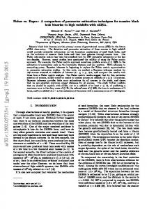
We used the Runge-Kutta 4th order method to compute the ˆ parameter vector θ(t). C. Multi-estimator (ME) The multi-estimator (ME) method is a part of supervisory control originally proposed by Morse [15], [16]. The goal of supervisory control is the same as that of conventional adaptive control: to control uncertain systems by adaptation. The main difference is that conventional methods design a controller and update unknown parameters in a continuous way, while supervisory control does so by means of logic-based switching. A large number of candidate controllers/estimators are prepared in advance, and switching among them is automatically done by a supervisor. Supervisory control consists of three components: multi-estimator E, monitoring signal generator M, and switching logic S.
(1)
where f is the interaction force between the robot and the environment, and b, k, and x are damping, stiffness, and displacement of the environment, respectively. Let us define a regression vector, ϕ(t) = [x(t), ˙ x(t)] T , and a parameter T vector, θ = [b, k] , so that (1) is written as: T
where β (0 < β ≤ 1) is a forgetting factor and the subscript n denotes t = nT .
x∙ x x∙ x
E fp1 = b1x∙ + k1x
fp1 +
fp2 = b2x∙ + k2x
fp 2 +
M
f ep1
|| ||
μp1
ep2
|| ||
μp2
|| ||
μpm
f
S
σ
(2)
A. Recursive least-squares (RLS) Recursive least-squares (RLS) minimizes the mean square ˆT value of the model error at every time step. Let θˆ = [ˆb, k] where ˆb and kˆ are the estimates of b and k, respectively. The parameter vector is calculated every sample time as [10]: � � θˆn = θˆn−1 + Ln fn − ϕTn θˆn−1 (3) � � � −1 Ln = Pn−1 ϕn β + ϕTn Pn−1 ϕn where (4) Pn = β −1 [I − Ln ϕTn ]Pn−1
x∙ x
fpm = bmx∙ + kmx
Fig. 1.
fpm +
f epm
Multi-estimator design for our framework
Fig. 1 shows a block diagram of an ME for our system. There are m distinct candidate estimators. Each estimator accepts two signals, x˙ and x, and yields an estimated output
fpi (1 ≤ i ≤ m). The estimated output is compared to the measured output f and we have an estimation error of epi = fpi − f .
(10)
The estimation error is passed to the monitoring signal generator, M, which outputs a monitoring signal defined as � µpi (t)
=
t 0
e−2λ(t−τ ) �epi (τ )�2 dτ ,
(11)
where λ ≥ 0 [9]. The switching logic, S, chooses an estimator that yields the minimum amount of monitoring signal. In the original idea, the switching logic outputs a signal, σ, that is used to define the control signal, u. We only pursue the estimation part in this paper, and thus the output from the switching logic is not used to design the controller.
1) One of the estimators is same as the plant: Lemma 1: Assume we have the true estimator that is exactly the same as the plant. There exist estimators that produce zero error and thus zero monitoring signal for all t if and only if x(t) = x 0 exp(− ∆k ∆b t), where ∆b and ∆k are defined later. Proof: [Necessary condition] Given the plant: f = bx+ ˙ kx, we have the true estimator f pα = bα x˙ + kα x that is exactly the same as the plant, i.e. (b α , kα ) = (b, k). The estimation error e pα is always zero, and thus µ pα (t) = 0 for all t from (11). Suppose we have another estimator, f pβ = bβ x˙ + kβ x where bβ = ∆b + b and kβ = ∆k + k, that is distinct from the true estimator but produces the same amount of monitoring signal, i.e. µ pβ (t) = µpα (t) for all t. In order to have µ pβ (t) = 0 for all t, epβ (t) = 0 for all t. Then, epβ = fpβ − f = ∆bx˙ + ∆kx = 0 .
III. PARAMETER CONVERGENCE For estimated parameters to converge to “true” values, the input signal needs to be rich enough to excite all the modes of the plant. This property is called persistent excitation [17] and referred to as PE. If the regression vector ϕ is PE, a matrix Pn in (3) is nonsingular and thus estimated parameters will be consistent for RLS [10]. In the case of AI, if ϕ is PE, the differential equation (9) is uniformly asymptotically stable [17]. The regression vector is therefore required to be PE for RLS and AI to guarantee the parameter convergence. As explained in the previous section, our ME technique finds the best estimator based on the force estimation error. Although the estimated parameters are not guaranteed to converge to the true values, the ME algorithm does not need persistently exciting signals. However, this does not mean it always chooses the best estimator for any type of input signal. If there are multiple unknown parameters, a parameterization redundancy problem may occur.
A. Parameterization redundancy A major question in our multi-estimator design is whether there exists redundancy of parameterization since we have two unknown values in the plant. With multiple unknown parameters, even if a true estimator (which is exactly the same as the plant) exists, there might be an estimator with a wrong set of estimated parameters that still produces the same amount of monitoring signal as the true estimator. If so, the switching logic may choose the wrong parameterization. On the other hand, if no true estimator exists, there might also be multiple estimators that produce the same amount of monitoring signal. If so, the switching logic could not choose one. In the following two subsections, the parameterization redundancy problem is discussed assuming no noise or disturbance to the system.
If x(t) is constant and equal to zero, the above equation always holds. This is trivial, and the condition of x = 0 is ignored. If ∆b �= 0, x˙ = −
∆k x, ∆b �
∆k t x(t) = x0 exp − ∆b
� .
(12)
If ∆b = 0, ∆k also needs to be zero, which contradicts the assumption that the two estimators are distinct. [Sufficient condition] Given x = x 0 exp(− ∆k ∆b t) where x(0) = x0 and we have two distinct estimators, the true estimator α and the other one β, as defined before. The estimation error e pβ is epβ = ∆bx˙ + ∆kx
∆k ∆k � − ∆k t e ∆b + ∆kx0 e− ∆b t = ∆b x0 − ∆b = 0. Since the error is zero, this results in µ pβ (t) = 0 for all t. Therefore, redundancy exists if and only if (12) is satisfied. 2) None of the estimators is same as the plant: Lemma 2: If no estimator is exactly the same as the plant, there exist estimators that can produce the same amount of error and thus the same amount of monitoring signal for t ∈ [tp , tq ] for the following three cases: (∆b γ� , ∆kγ ) = � ∆k(1) γ −∆kε (−∆bε , −∆kε ); (2) x(t) = x0 exp − ∆bγ −∆bε t ; and (3) � ∆k +∆k � x(t) = x0 exp − ∆bγγ +∆bεε t and ∆bγ ∆kε = ∆bε ∆kγ . Proof: Given the plant: f = bx˙ + kx, we do not have any estimator that is exactly the same as the plant. Assume we have two distinct estimators f pγ = bγ x˙ + kγ x and fpε = bε x˙ + kε x. The estimation errors are epγ = ∆bγ x˙ + ∆kγ x , epε = ∆bε x˙ + ∆kε x .
Suppose there are conditions that lead to µ pγ = µpε for some t ∈ [tp , tq ]. This requires that the two estimators produce the same amount of estimation error for t ∈ [t p , tq ]. Since any 2-norm is greater than or equal to zero and e p is scalar in our case, �epγ �2 = �epε �2
⇐⇒ �epγ � = �epε � , ⇐⇒ |epγ | = |epε | .
Thus, the condition can be simplified to ∆bγ x˙ + ∆kγ x = ±(∆bε x˙ + ∆kε x)
(13)
The condition of x = 0 is also trivial in this case. (i) If ∆bγ x˙ + ∆kγ x = ∆bε x˙ + ∆kε x (13) ⇒ (∆bγ − ∆bε )x˙ + (∆kγ − ∆kε )x = 0 If ∆bγ �= ∆bε , the solution is � � ∆kγ − ∆kε t x(t) = x0 exp − ∆bγ − ∆bε
(14)
If ∆bγ = ∆bε , it results in ∆kγ = ∆kε , which contradicts the distinction of the two estimators. (ii) If ∆bγ x˙ + ∆kγ x = −(∆bε x˙ + ∆kε x) (13) ⇒ (∆bγ + ∆bε )x˙ + (∆kγ + ∆kε )x = 0
If ∆bγ + ∆bε �= 0, on the other hand, the solution is � � ∆kγ + ∆kε t x(t) = x0 exp − ∆bγ + ∆bε
The main goal of this paper is to find out what needs to be considered to estimate unknown mechanical properties of the environment online. The experiments consists of two parts: (1) data acquisition and (2) parameter estimation. We did not update a controller based on the online estimation. This allows us to separate the two procedures. However, we could have done the both tasks simultaneously during telemanipulation, as would be desirable in real applications. A. Design 1) Materials: Three soft cubes were used as artificial tissues for the experiments. The dimensions of the soft cubes are 50mm × 50mm × 40mm. They each have a different stiffness: soft (Cube 1), medium (Cube 2), and hard (Cube 3). All the cubes are made of silicone rubber. There are no official data showing the damping and stiffness values of the soft cubes. 2) Control conditions: The input signal to the system needs to be PE for some estimation algorithms in order to guarantee the parameter convergence. To test whether additional reference forces other than the one generated by the operator are needed, we used three types of control conditions: (i) teleoperation without PE, (ii) teleoperation mimicking PE by the operator, and (iii) autonomous control with PE. 3) Estimation methods: Three estimation methods were applied: recursive least-squares (RLS), adaptive identification (AI), and multi-estimator (ME). B. Experimental setup
If ∆bγ + ∆bε = 0, ∆kγ + ∆kε = 0. Therefore, (∆bγ , ∆kγ ) = (−∆bε , −∆kε )
IV. E XPERIMENTS
Environment
Metal Plate
Master
(15)
Metal Wall
Slave
(16)
under the condition of ∆b γ ∆kε = ∆bε ∆kγ . B. Physical interpretation of the redundancy conditions When the plant is given as f = bx˙ + kx, regardless of the existence of the true estimator, redundancy exists. However, if we consider the physical meaning of the conditions that lead to redundancy, conditions (12), (14), and (16) would not occur. To meet these conditions, the user would have to make the slave go exponentially to infinity or zero. The condition (15), on the other hand, could occur. The physical interpretation of the condition (15) is that we may overestimate or underestimate environment parameters by the same amount. Hence, we cannot say if either model is closer to the plant unless we have another criterion to choose a desired estimator. Therefore, in our framework, the ME method practically chooses the best approximated model.
Fig. 2. Experimental setup of 1-DOF teleoperation system and a soft cube as the environment
Data were acquired using a 1-DOF telemanipulation system, as shown in Fig. 2. A force sensor is attached on the master robot to measure the input force from the operator. The input force is used to calculate the master velocity that is used to command the slave velocity. A square metal plate is attached at the tip of the slave. It covers all the surface area of the environment. The soft cube is gently attached to the metal wall by a tape, and it is always in contact with the slave. This setting allows us to use the simple environment model (1). The operator only had direct visual feedback and received no force feedback from the environment. The operator was asked to palpate a soft cube with arbitrary motion (teleoperation without PE) or trying to make a sinusoidal movement with a constant frequency and amplitude (teleoperation
C. Estimation setup Prior to the estimation, some parameters are tuned in advance by trial and error. The initial values of the covariance matrix P of RLS (4) are set: 100 0 (17) P0 = 0 100
(19)
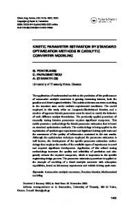
D. Results Once the data acquisition task was performed, unknown parameters and interaction forces were estimated by the parameter identification algorithms. Fig. 3 shows sample profile of estimated parameters for each algorithm. The sample plots shown in Fig. 3 were acquired using teleoperation without PE with Cube 1 as the plant. All the estimation results are summarized in Table I. Estimated parameters for AI and ME are averaged over an experimental period of 10 seconds. An average force error ef is defined as follows: n � � � �fk − fˆk �/nT k=0
where f is measured force and fˆ is estimated force. The average force error e f is different from the estimation error epi (10), which is defined only for the multi-estimator.
Displacement [mm] Velocity [mm/s]
(18)
where 1 ≤ i ≤ 41 and 1 ≤ j ≤ 193. There are 41 and 193 candidates for damping and stiffness, respectively, and thus 7913 candidate estimators are available in total, i.e. m = 7913 in Fig. 1. Note that, unlike AI, which requires the different adaptation gain depending on the cube as seen in (18), the same candidate estimators were used for all the cubes for ME. The initial parameters guess for both RLS and AI is (b, k) = (0, 0), which is a common assumption for parameter estimation. The forgetting factor λ in (11) should be set very small if the environment is linear and uniform. In our experiments, contrary to the model, the material is not linear, and thus mechanical properties are not uniform. Therefore, λ = 10 is chosen. For RLS, we chose β = 0.98 so that e −2λt ≈ β with an update rate of 1kHz.
ef =
10 8 6 4 2 3000 2500 2000 1500 1000 RLS AI ME
500 0
5
6
7
8
9
10
11
12
13
14
15
100
where diag is a 2 × 2 diagonal matrix. For ME, damping and stiffness values of candidate estimators are chosen as: bi ∈ [−500, −475, −450, · · ·, 450, 475, 500] kj ∈ [1500, 1700, 1900, · · ·, 39500, 39700, 39900]
12
Time [s]
Estimated Damping [Ns/m]
and the gain matrix in (8) for AI is chosen as: ⎧ ⎨ Cube 1: diag (2000, 1.2 × 10⁵ ) Cube 2: diag (5000, 5.0 × 10⁵ ) Γ= ⎩ Cube 3: diag (50000, 107)
14
Estimated Stiffness [N/m]
mimicking PE). Autonomous control with PE was completed without any human operator, and sinusoidal force input was chosen as a typical PE. There are three soft cubes and three control methods prepared, and thus nine different conditions exist.
50 0 −50 −100 500 250 0 -250 −500
RLS AI ME
5
6
7
8
9
10
11
12
13
14
15
Time [s]
Fig. 3. Comparison of estimated parameters: recursive least-squares, adaptive identification, and multi-estimator. The upper figure shows estimated stiffness with displacement profile and the bottom shows estimated damping with velocity profile.
V. D ISCUSSION There were three main factors in the experiment: cube type (soft, medium, and hard), system control condition (teleoperation without PE, teleoperation mimicking PE, and autonomous with PE), and estimation algorithm (RLS, AI, and ME). In this section, we will consider the role of each factor in the accuracy and speed of estimation. Our discussion will be limited to the stiffness estimation because the damping of the cubes was so low as to have a negligible effect on total force. In addition, some of the estimated damping values are negative, which should not occur for a physical object. This may be due to limitations of the model or noise in the sensed force and velocity calculated from encoders. A. Comparison of the cube types The stiffness of the cubes did not affect the accuracy or rise time of any of the estimation algorithms. Fig. 4 gives the estimation response for each of the estimation methods done online. Fast convergence is obtained for all three online estimation methods. The oscillation is desirable because the
TABLE I E STIMATED PARAMETERS OF THE ENVIRONMENT AND AVERAGE FORCE ERRORS FOR EACH ESTIMATION ALGORITHM Control Method
Estimation Algorithm RLS AI ME RLS AI ME RLS AI ME
Teleoperation without PE Teleoperation mimicking PE Autonomous Control with PE
Cube 1 ˆ [N/m] k 2229.2 2212.7 2202.7 2372.6 2310.0 2338.0 2085.1 2093.3 2100.1
ˆb [Ns/m] -12.5 9.2 -16.8 -19.5 23.5 -42.5 -7.3 1.2 35.1
ef [N] 0.34 0.97 0.49 0.39 1.02 0.57 0.10 0.72 0.21
3000
ˆb [Ns/m] -492 13 -367 -429 608 -226 -441 101 -284
Cube 3 ˆ [N/m] k 33034 33207 33276 28308 31099 29288 19813 20187 19850
ef [N] 0.99 1.53 1.01 0.53 2.34 0.57 0.76 1.47 0.77
2000
RLS AI ME
0
1000
Cube 1
Estimated Stiffness [N/m]
1000
Estimated Stiffness [N/m]
ef [N] 0.25 0.90 0.38 0.56 1.22 0.57 0.34 1.11 0.31
3000
2000
6000 4000
RLS AI ME
2000 0 4
Cube 2 ˆ [N/m] k 5235.1 5046.5 5158.1 4857.8 5113.0 4901.0 4626.6 4613.7 4605.3
ˆ b [Ns/m] -28.7 108.9 -74.3 -50.1 36.0 -53.9 -52.1 -41.3 -50.6
x 10
Cube 2
4
0
RLS AI ME
Teleoperation without PE
RLS AI ME
Teleoperation mimicking PE
3000 2000 1000 0 3000
3
2000 2
RLS AI ME
1 0 5
6
7
8
1000
Cube 3 9
10
11
12
13
14
15
Time [s]
0 5
6
7
RLS AI ME 8
Autonomous control with PE 9
10
11
12
13
14
15
Time [s]
Fig. 4. Estimated stiffness for Cubes 1, 2, and 3. The control method was teleoperation without PE. For all the cubes, all three estimation methods show the quick parameter convergence.
Fig. 5. Estimated stiffness under the control condition of teleoperation without PE, teleoperation mimicking PE, and autonomous control with PE. The plant was Cube 1.
stiffness of the environment varies with penetration depth. More force error is observed as the stiffness of the cube increases (Table I). For increased interaction forces, the errors between the estimated forces and the measured forces naturally become larger.
C. Comparison of the estimation algorithms
B. Comparison of the control conditions The control conditions also had little effect on estimation performance. Fig. 5 shows the estimation response for each of the estimation methods under the different control conditions. In our experimental settings, even without having PE, all online estimation algorithms converge rapidly. Comparing the average force errors in Table I, autonomous control with PE shows smaller errors than the other control methods. This is partly because the penetration depth by autonomous control was smaller than the other control methods. With small penetration, the estimated stiffness is small, and thus the interaction force is also small. Since the material is nonlinear, the penetration depth plays an important role for comparison. Further research is required to find the role of control methods on estimation performance. This will be especially important for very viscoelastic or massive environments.
The estimation algorithms can be compared in terms of speed and accuracy in Figs. 4 and 5, and Table I. We also discuss the practical aspects of each estimation technique. Surgeons usually palpate the tissue only once or a few times at one location, then do it at another. One palpation takes about 1 second or more. From Figs. 4 and 5, we can see that the rise time of the three estimation techniques is up to 0.6s and thus short enough to estimate the stiffness by one palpation. Although AI may appear to converge more slowly than the other two methods, a closer initial guess and better adaptation gain would improve the rise time. It is interesting to see that there is no rise time for ME since it does not need initial estimation guess and can choose the best approximated estimator quickly. Regarding the accuracy of the estimation, RLS showed the lowest force estimation error in most cases. Because of the faster convergence of ME, it would be expected to have lower estimation error than RLS. However, the lack of ability to converge to the true values would yield some errors even at the steady state while RLS shows zero error. This made RLS slightly more accurate than ME. In our experimental setup, we used a open-loop control:
the interaction force between the slave and the environment was not fed back to the operator. In a closed-loop system, adaptive control would be easy to implement since it uses AI to estimate the unknown environment parameters that can be used to update a controller [8], [14]. However, the choice of the adaptation gain is a key to obtain good estimation results (convergence and accuracy). Therefore, it may not be an ideal method for surgical applications since the environments encountered in surgery are inhomogeneous and thus it is quite difficult to tune the adaptation gain in advance. RLS showed fast convergence as well as accurate force estimation. With persistent excitation, the parameter convergence is guaranteed. Moreover, it is easy to implement: only simple initial parameter setting is required. So, RLS can be expected to work well with minimum amount of work for the tissue property estimation. In a closed-loop system, a controller needs to take into account the updated environment model to improve transparency and stability of the teleoperation system, which has not been established well unlike adaptive control. As well as RLS, ME also requires less tuning. In [2], Kalman Active Observer is able to differentiate soft and stiff objects, but there are numbers of parameters to be carefully tuned in advance. While the gain matrix of AI (18) needed to be changed depending on the stiffness of the cube, the same candidate estimators for ME (19) were used for all the three cubes. The forgetting factor should be considered based on whether the material is uniform. Compared to tuning gains in adaptive identification algorithm, this is much less complicated. The stability of a closed-loop multiestimator/controller system is slightly complicated [15], [16]. The dwell time to switch controllers has to be considered. VI. C ONCLUSIONS This work presents three parameter identification techniques (recursive least-squares, adaptive identification, and multi-estimator) to estimate unknown environment parameters. We first show that the multi-estimator chooses the best estimator among the candidates by theoretical analysis. Using a teleoperation system and artificial tissues, real interaction data were obtained. There are three system control conditions: teleoperation without persistent excitation, teleoperation mimicking persistent excitation, and autonomous control with persistent excitation. Three cubes having different stiffness are chosen as an environment. Only the choice of the estimation algorithm has an effect on estimation performance. For online parameter estimation for surgical applications, either RLS or ME would be appropriate. As future work, we plan to apply an online estimation algorithm to our engineering version of the da Vinci surgical system [12] and perform experiments with real tissues. Our eventual goal is to acquire patient model online during robot-assisted surgery so that the model can be used during and after a procedure to improve teleoperation transparency, medical diagnosis, and surgical simulation.
R EFERENCES [1] M. B. Colton and J. M. Hollerbach. Identification of nonlinear passive devices for haptic simulations. In WHC ’05: Proceedings of the First Joint Eurohaptics Conference and Symposium on Haptic Interfaces for Virtual Environment and Teleoperator Systems, pages 363–368, 2005. [2] R. Corteso, J. Park, and O. Khatib. Real-time adaptive control for haptic telemanipulation with kalman active observers. IEEE Transactions on Robotics, 22(5):987–999, 2006. [3] R. Corteso, W. Zarrad, P. Poignet, O. Company, and E. Dombre. Haptic control design for robotic-assisted minimally invasive surgery. In IEEE International Conference on Intelligent Robots and Systems, pages 454–459, 2006. [4] N. Diolaiti, C. Melchiorri, and S. Stramigioli. Contact impedance estimation for robotic systems. IEEE Transactions on Robotics, 21(5):925–935, 2005. [5] D. Erickson, M. Weber, and I. Sharf. Contact stiffness and damping estimation for robotic systems. The International Journal of Robotics Research, 22(1):41–57, 2003. [6] G. De Gersem, H. Van Brussel, and J. Vander Sloten. Enhanced haptic sensitivity for soft tissues using teleoperation with shaped impedance reflection. In World Haptics Conference (WHC) CD-ROM Proceedings, 2005. [7] B. Hannaford. A design framework for teleoperators with kinesthetic feedback. IEEE Transactions on Robotics and Automation, 5(4):426– 434, 1989. [8] K. Hashtrudi-Zaad and S. E. Salcudean. Adaptive transparent impedance reflecting teleoperation. In IEEE International Conference on Robotics and Automation, pages 1369–1374, 1996. [9] J. P. Hespanha, D. Liberzon, and A. S. Morse. Overcoming the limitations of adaptive control by means of logic-based switching. Systems & Control Letters, (49):49–65, 2003. [10] L. Ljung. System Identification: Theory for the User. Prentice-Hall, 1987. [11] L. J. Love and W. J. Book. Environment estimation for enhanced impedance control. In IEEE International Conference on Robotics and Automation, pages 1854–1858, 1995. [12] M. Mahvash, J. Gwilliam, R. Agarwal, B. Vagvolgyi, L.-M. Su, D. D. Yuh, and A. M. Okamura. Force-feedback surgical teleoperator: Controller design and palpation experiments. In 16th Symposium on Haptic Interfaces for Virtual Environments and Teleoperator Systems, pages 465–471, 2008. [13] H. Mayer, I. Nagy, A. Knoll, E. U. Braun, R. Bauernschmitt, and R. Lange. Haptic feedback in a telepresence system for endoscopic heart surgery. Presence: Teleoperators and Virtual Environments, 16(5):459–470, 2007. [14] S. Misra and A. M. Okamura. Environment parameter estimation during bilateral telemanipulation. In 14th Symposium on Haptic Interfaces for Virtual Environments and Teleoperator Systems, pages 301–307, 2006. [15] A. S. Morse. Supervisory control of families of linear set-point controllers — Part 1: Exact matching. IEEE Transactions on Automatic Control, 41(10):1413–1431, 1996. [16] A. S. Morse. Supervisory control of families of linear set-point controllers — Part 2: Robustness. IEEE Transactions on Automatic Control, 42(11):1500–1515, 1997. [17] K. S. Narendra and A. M. Annaswamy. Stable Adaptive Systems. Dover Publications, Inc., 2005. [18] H. Seraji and R. Colbaugh. Force tracking in impedance control. IEEE Transactions on Robotics, 16(1):97–117, 1997. [19] S. K. Singh and D. O. Popa. An analysis of some fundamental problems in adaptive control of force and impedance behavior: Theory and experiments. IEEE Transactions on Robotics and Automation, 11(6):912–921, 1995. [20] X. Wang, P. X. Liu, D. Wang, B. Chebbi, and M. Meng. Design of bilateral teleoperators for soft environments with adaptive environmental impedance estimation. In IEEE International Conference on Robotics and Automation, pages 1127–1132, 2005.