Techniques for fast simulation of models of highly

246

IEEE TRANSACTIONS ON RELIABILITY, VOL. 50, NO. 3, SEPTEMBER 2001

Techniques for Fast Simulation of Models of Highly Dependable Systems Victor F. Nicola, Perwez Shahabuddin, and Marvin K. Nakayama

Abstract—With the ever-increasing complexity and requirements of highly dependable systems, their evaluation during design and operation is becoming more crucial. Realistic models of such systems are often not amenable to analysis using conventional analytic or numerical methods. Therefore, analysts and designers turn to simulation to evaluate these models. However, accurate estimation of dependability measures of these models requires that the simulation frequently observes system failures, which are rare events in highly dependable systems. This renders ordinary simulation impractical for evaluating such systems. To overcome this problem, simulation techniques based on importance sampling have been developed, and are very effective in certain settings. When importance sampling works well, simulation run lengths can be reduced by several orders of magnitude when estimating transient as well as steady-state dependability measures. This paper reviews some of the importance-sampling techniques that have been developed in recent years to estimate dependability measures efficiently in Markov and non-Markov models of highly dependable systems. Index Terms—Highly dependable system, importance sampling, Markov chain, simulation, steady-state dependability measure, transient dependability measure.

ACRONYMS1 BFB BLBLR BLBLRC BLR BRE CLT CTMC DTMC GSMP i.i.d. IS MC MSDIS MTBF MTTF

balanced failure biasing balance over links BLR BLBLR with cuts balanced likelihood ratio bounded RE central limit theorem continuous-time MC discrete-time MC generalized semi-Markov process -independent and identically distributed importance sampling Markov chain measure-specific dynamic IS mean time between failures mean time to failure

Manuscript received November 1, 1998; revised June 6, 2000. This work was supported in part by the US National Science Foundation under Grants DMI9625297, DMI-9624469, and DMI-9900117. Responsible Editor: C. Alexopoulos V. F. Nicola is with Telematics Systems and Services, Department of Electrical Engineering, University of Twente, Enschede, The Netherlands. P. Shahabuddin is with Columbia University, New York, NY 10027 USA (e-mail: [email protected]). M. Nakayama is with the Department of Computer and Information Science, New Jersey Institute of Technology, Newark, NJ, USA. Publisher Item Identifier S 0018-9529(01)11169-3. 1The

singular and plural of an acronym are always spelled the same.

NHPP pdf r.v. RE RP SAVE TH TRR VRR

nonhomogeneous Poisson process probability density function random variable relative error repair person system availability estimator time horizon total effort reduction ratio variance reduction ratio. I. INTRODUCTION

H

IGH dependability requirements of today’s critical and/or commercial systems often lead to complicated and costly designs. The ability to predict relevant dependability measures for such complex systems is essential, not only to guarantee high levels of dependability during system operation but also to improve the cost-effectiveness during system design and development. Several measures are commonly used for assessing the dependability of a system, and the choice of the particular dependability measures used to evaluate a particular system depends on the intended operation and the environment of such a system. For example, mission-oriented systems are often evaluated using transient measures, such as system reliability (probability that the system is operational during the entire mission time). Given that the system is initially in an operational state, MTTF is the mean time to the first system failure; this is another measure of interest for mission-oriented systems. On the other hand, MTBF is the mean time between subsequent system failures in steady-state. MTBF and the steady-state availability (fraction of time the system is operational in the long run) are often used for evaluating continuously operating systems. Fault-tolerance and recovery techniques are frequently used in the design of complex systems to enhance their dependability. As a consequence, very high reliability/availability requirements of systems can now be sustained. However, the performance of continuously operating systems can be degraded/upgraded due to load surges or reconfigurations after failures/repairs. In other words, the performance level of degradable/repairable systems is changing with time in response to internal or external events. To evaluate these systems properly, there is a need for measures that combine performance and reliability/availability aspects. Such measures were first introduced in [74], and were termed “performability” measures. An example of such a measure is the distribution (or -expectation) of cumulative performance in a given interval of time. A special case of this measure is the distribution (or

0018–9529/01$10.00 © 2001 IEEE

NICOLA et al.: TECHNIQUES FOR FAST SIMULATION OF MODELS

-expectation) of interval availability, which is the fraction of time the system is operational (regardless of performance) during a given interval of time. The distribution of interval availability (or guaranteed availability [48]) is a relevant attribute of continuously operating systems, because it gives the probability that the system is operational for more than a specified fraction of a given interval of time. For example, one might be interested in computing the probability that the system is unavailable for more than 0.1% of the time in 1 year of system-operation. A. Numerical Evaluation of Dependability Measures Researchers have long been aware of the importance and necessity of developing techniques and tools to evaluate highly dependable systems effectively. Most of the efforts are limited to analytic or numerical solutions, usually restricted to Markov (less often, semi-Markov) models. For a more detailed discussion on performability measures and state-of-the-art techniques for their evaluation, see [23]. The applicability of these techniques, however, is quickly hindered by practical problems, such as state-space explosion and/or the inadequacy of Markov or semi-Markov representations of real systems. Because the number of states in Markov models usually grows exponentially with the number of system-components, and because of storage and computational limitations, only relatively small systems can be analyzed using numerical solution techniques. Several techniques have been proposed and, if applicable, can help to reduce the state-space of large Markov models. For example, exact lumping [45], [84], or approximations obtained by truncation and bounding [76], are used. However, even for a moderately-sized system, the corresponding Markov model can be “stiff”2 (usually when transition rates are of different orders of magnitude), leading to difficulties when using numerical solvers [92]. Behavioral decomposition [9] and iterative decomposition/aggregation techniques [19] are among several techniques that can help overcome “stiffness” of Markov models. B. Effective Simulation When conventional analytic/numerical methods are no longer feasible, analysts often turn to computer simulation, with the obvious advantages of flexible representation of complex systems at the desired level of abstraction and low storage requirements. However, the accurate estimation of dependability measures using simulation requires frequent observations of the system-failure event, which by definition are rare events in highly dependable systems. This renders conventional (ordinary) simulation impractical for evaluating such systems [30]. To attack this problem, in recent years, there have been considerable and successful efforts to develop fast simulation techniques based on IS [41], [51]. The basic idea is quite simple: simulate the system using new probability-dy2A stochastic process is “stiff” when it contains 2 essentially different types of transitions, slow and rapid [66, ch. 8]. Highly dependable systems consisting of highly dependable components fit this description because, typically, the component lifetimes are very long, whereas repairs take only a short time to complete.

247

namics (different from the original probability-dynamics of the system), so as to increase the probability of typical sequences of events leading to system failure. For example, in a redundant system with 2 components, accelerating the component#2 failure while component#1 is being repaired, typically increases the probability of another component failure, which would lead to system failure. The obtained measure in a given observation (a sample path of a simulation trial) is then multiplied by a correction factor called the “likelihood ratio” to yield a -unbiased estimate of the measure. This factor is the ratio of the probabilities (likelihoods) of the sample path in the original and modified systems, respectively; its computation is straightforward and can be done recursively at simulation event times. Appropriate and careful choice of the new underlying probability dynamics of the simulated system can yield an appreciable reduction in the variance of the resulting estimate, which implies appreciable reduction in the simulation time needed to achieve a specified precision. Also, the new probability dynamics should be easy to implement. For a fixed run-length, ordinary simulation produces estimates with RE (a constant times the coefficient of variation of the estimate) that tends to infinity as the probability of the rare event tends to zero. An “effective” heuristic for IS is one that, for a fixed run-length, produces estimates with a RE that remains bounded as the probability of the rare event tends to zero. However, BRE is an asymptotic property, and in practice, even if an IS heuristic possesses this property, the amount of simulation effort required to achieve a given precision can still be large. Also, the BRE property might not ensure a variance reduction relative to ordinary simulation for many types of highly dependable systems (e.g., systems with an appreciable level of redundancies) whose parameters fall in the practical range; it only guarantees that as the event of interest becomes rarer, the -expected amount of simulation effort remains bounded by a constant (in contrast to ordinary simulation where this effort tends to infinity), but the bound can be large. C. This Work This paper reviews some of the recent IS techniques developed for the efficient estimation of transient and steady-state dependability measures in Markov and non-Markov models of highly dependable systems.3 Parts of [53] also review some IS techniques for the simulation of dependability measures, with emphasis on the underlying mathematical ideas needed to establish their theoretical properties; thus, it is more suitable for researchers. This paper presents a comprehensive and less mathematical treatment of the subject; therefore, it is more suited for reliability practitioners, and requires only a basic understanding of probability and statistics. There are two main ways in which a system can be made highly dependable in a cost-effective manner. 1) Use components that are “highly reliable” and have “low” built-in redundancies in the system. Examples of these are computer systems where the main components (e.g., processors) fail rarely. 3Preliminary versions of some parts of this review have appeared in [80] and [100].

248


2) Build “significant” redundancies in the system and use components that are just “reliable” instead of “highly reliable.” (The distinction is clearer when some examples are examined later in the paper.) There might also be a third way: Use “unreliable” components but have “very high” built-in redundancies in the system. Examples are more difficult to find in practice. Much of the recent research work on effective simulation of highly dependable systems has been done for systems that fall in categories 1 and 2, and this paper mainly covers those. The focus in this paper is on “dynamic” systems (systems that change over time), in contrast to “static” systems. An example of a static system is a 2-terminal reliability network with -independent components and no repairs (strictly speaking, there can be repairs as long as they do not create -dependencies among components). See, [69], [70], [95] for fast simulation methods for such systems. Section II formally describes the wide class of systems for which these IS techniques are designed, and reviews the basic idea of IS. Section III discusses IS techniques for estimating dependability measures in Markov models. “Markov” implies that all failure, repair, and other underlying distributions in the system are exponential, so that it can be modeled by a CTMC. Some work is reviewed on the estimation of derivatives with respect to model parameters (e.g., component failure rates) for various steady-state and transient measures in these models. This work is of much interest, because it can be used to identify systemcomponents that might need improvement and to optimize systems. Section IV considers the estimation of dependability measures for models in which the failure and repair times are not exponentially distributed. Because these types of system can no longer be directly modeled as a MC, they are called “non-Markov models.” A mathematical framework for studying such systems is the GSMP; see [37] for a formal development of GSMP. The general theory of IS for discrete-event systems (without discussing the particular changes of measures for specific models) is in [37], [41]. For the IS heuristics discussed in this paper, some empirical studies have been presented in the literature, and many of these methods are provably effective. In both Markov and non-Markov models, the concern is estimation of • transient measures, such as system unreliability, -distribution and -expectation of interval unavailability, • steady-state measures, such as steady-state unavailability and MTBF. Although MTTF is in fact a transient measure, for regenerative models it can be represented as a ratio of 2 -expectations of regenerative-cycle-based quantities that can be estimated using the regenerative method of simulation. Thus MTTF is included in discussions of steady-state measures. Section V discusses ongoing work and directions for future research.

D. Related Work and Software IS can be applied, not only for estimating dependability measures of reliability systems, but for estimating buffer-overflow probabilities in queuing systems and networks [18], [28], [91], [96], [107]. Applications to communication systems are of particular interest [4], [15], [113], [67]. The IS techniques used in this setting are often based on the theory of large deviations. A survey on existing techniques is in [53]. An approach, other than IS, based on “fault-injection” is used in [75] to speed up steady-state simulations involving rare (failure) events in communication systems. The method assumes knowledge of the frequency of the “rare failure event” and exploits the fact that, except for relatively short periods after failures, the system is operating normally in a failure-free environment. Fault-injection is used to obtain an accurate estimate of the performance measure of interest during periods affected by the failure. This estimate is appropriately combined with an accurate estimate under failure-free environment (with no rare events) to yield an overall steady-state estimate of the dependability measure. Another method to simulate rare sample paths is to use the technique of “splitting” sample paths. Splitting for rare-event simulation was originally discussed in [62] in the context of estimating rare particle transmission probabilities in physics [51]. Since then, it continues to be an active area of research in that field [24]. Variations of this technique for steady-state rare-event estimation in stochastic service systems seem to have been first done in [6], [7], and later in [57] (see [14] for a related idea); a variation for transient rare-event estimation in stochastic service systems is in [65]. It was revisited in [110], [111], [112] for estimating probabilities of rare events in computer and communication systems; the version of the technique used in these papers was called “RESTART.” Some of the most recent versions/implementations of the technique are in [29], [35], [43], [52]. The basic idea behind the splitting technique is explained here. The goal typically is to estimate some performance measure that is “associated with” visiting some set of states of the state space of the stochastic process, and the set is visited only rarely. For example, compute the probability of a buffer overflow, where corresponds to states in which the buffer content has reached its capacity. In ordinary simulation, the stochastic process being simulated spends a lot of time in regions of the state space that are “far away” from the interesting rare set (regions from where the chance of entering the rare set is extremely low). In one version of splitting, a region of the state space that is “closer” to the rare set is defined. Each time the process enters this region from the “far away” region, many identical copies of the process are generated. Each of the split copies is simulated until the process exits back into the “far away” region. From there on, only one of the split copies is continued until another entrance into the “closer” region. This way gives more instances of the stochastic process spending time in the “closer” region where the rare event is more likely to occur. The idea can be extended to: instead of just 2 regions, use multiple regions of slowly increasing degrees of rarity. Reference [35] describes a


unifying class of models and implementation conditions under which this type of multi-level splitting is provably effective for steady-state rare-event simulation. Related work is in [33], [34]. The method of splitting has also been used and analyzed in contexts other than rare-event simulation, e.g., [73]. There are a few software-based modeling tools which use rare-event simulation techniques for dependability evaluation. SAVE [45] is a software package that consists of a high-level modeling language that can be used to specify the model of interest. From this specification and Markov assumptions on the lifetime and repair-time distributions, the detailed Markov chain is derived. It is then solved for dependability measures using either numerical (nonsimulation) or simulation methods. A recent version of SAVE [8] incorporates the IS technique, BFB (as described in Section III-A) at the MC level to estimate dependability measures efficiently. Another software package where IS is used is ULTRASAN [20]. In ULTRASAN, the high-level modeling construct of stochastic activity networks is used to specify the model of interest. Again, from this specification, the detailed stochastic process is derived and solved for performance/dependability measures of interest, using either numerical (nonsimulation) MC methods or simulation methods. In recent versions of ULTRASAN [89], [90] an “IS governor” has been incorporated. Here, instead of the IS heuristic being built-in as in SAVE, one can choose and specify the IS change of measure at the stochastic activity network level. The RESTART version of the splitting method has also been implemented in ASTRO [112].

II. BACKGROUND Notation

RE

number of types of components number of components of type , number of operational components of type at time vector stochastic process state of the system at time stochastic process state space of subset of failure states in time to first system-failure probability under measure -expectation under measure variance under measure system unreliability at time indicator function of event convergence in distribution -normal distribution with mean , variance relative error of an estimator a sample path in the set of all of a stochastic process pdf of under measure likelihood ratio on .

249

A. Highly Dependable Systems This section discusses the broad class of highly dependable systems that can be described by SAVE [45] (basically, a generalized Machine Repairman Model). These models consist of multiple types of components, where each component can be in 1 of 4 states: • operational, • failed, • spare, • dormant. The first 3 of these states are self-explanatory. An operational component becomes dormant if its operation depends upon the operation of some other component and that other component fails. For example, a processor might not be operational unless its power supply is also operational; therefore, if the power supply fails, then the processor is dormant. In SAVE, different (exponential) failure rates can be specified for the operational, spare, and dormant states. The SAVE modeling language is also used to describe operational/repair dependencies among components (e.g., the operation/repair of a component depends on some other components being operational), as well as failure propagation (e.g., the failure of a component causes some other components to fail with given probabilities). The system is operational if certain combinations of components are operational. Unlike SAVE, in non-Markov models (Section IV) general failure and repair distributions are allowed. Also, there is a set of RP who repair failed components according to some reasonably arbitrary service (priority or nonpriority) discipline. To simplify the presentation, systems are considered in which each component is either operational or failed. (Unless otherwise specified, the results also apply to the more general models in the SAVE modeling language.) Section II-B briefly reviews the basic idea of IS and shows how (when applied appropriately) it could appreciably speed-up simulations involving rare events. For illustration, also consider estimating the system unreliability; however, the same concepts also apply to other dependability measures. B. Importance Sampling Consider a system with component-types. Each component is subject to failure and repair. , for all All components are operational at time 0: . All components are “new” at time 0. contains the information , but other inIn general, formation might be needed, e.g., the queuing of failed components waiting to be repaired and the remaining lifetimes and repair times of components when using distributions other than exponential. of the state space such that the There is some subset . system is failed at time if System unreliability is (1) TH.

250


The subscript denotes the original probability measure: the underlying original probability distributions governing the dynamics of the system. In a highly reliable system, for a sufficiently small , the : is rare. In ordinary (naive) simulation generate i.i.d. replications of from time 0 to time to obtain samples of , say, . Then

An -unbiased estimate of

The variance of

is

is

One measure of effectiveness of any new simulation algorithm is the VRR: ratio of the variance using ordinary simulation to that using the new simulation algorithm; in this case: is an -unbiased estimator of is

. The variance of this estimator

The VRR gives the ratio of the number of samples using ordinary simulation to that using the new algorithm so as to achieve the same RE. However this measure of effectiveness does not consider the effort (e.g., CPU time) required to simulate each sample under the two methods. Hence a more fair measure of effectiveness is the TRR: ratio of (the product of the variance and the effort per sample using ordinary simulation) to (that using the new simulation algorithm), [42]. The TRR gives the ratio of the total effort using ordinary simulation to that using the new algorithm so as to achieve the same RE. The main challenge in IS is to find a robust new probability measure that can be implemented in a computationally effi: cient manner such that

From the CLT as of

which is the relative half width of the 99% -confidence interval derived from the CLT approximation. For a fixed , the as . This is the main problem when using ordinary simulation to evaluate highly dependable systems. The goal of IS is to overcome this inherent difficulty. Notation another probability measure a sample path (of a replication) in the set of all possible sample paths of taking the system from time 0 to time pdf of according to

(3) Appreciable variance reduction from (3) is obtained if whenever

such that (4) is satisfied is usually very difficult Choosing because it involves each sample path. But the general intuition one obtains is that should be chosen to appreciable increase . At the same time one the probability of the rare event has to be very careful; choosing an arbitrary (but not suitable) that increases the probability of the rare event can lead to a substantial increase in variance. For highly dependable systems, try to come up with IS techniques that are “effective” (see Section I-B): techniques whose ) as the probRE remains bounded (implying that ability of the rare event tends to zero. This property has been established at least empirically (and, in many cases, also theoretically) for most of the IS techniques in this paper. However, as mentioned before, this does not always guarantee efficient simulation of systems with high redundancies.

(2) III. FAST SIMULATION OF MARKOV MODELS The only condition imposed on

is:

Notation

whenever Thus the system can be simulated using to obtain : ples of

i.i.d. sam.

(4)

,

collection of all (measurable) subsets of DTMC embedded on (when is a CTMC) generic states from the state space transition probability matrix of the DTMC


system state in which all components are operational time to first return of to state -cycle sample path between two successive entries to a subset of states system failure time in a regenerative-cycle, or -cycle steady-state unavailability of the system estimator of , original and IS probability measures of on IS probability measure under BFB variance of a ratio estimator; probability measures and are used to estimate the numerator and denominator, respectively failure biasing parameter transition probability matrix of the DTMC under BFB , failure, repair rates of component type parameter in the failure rate of component type failure rarity parameter exact asymptotic order of magnitude “distance” of state from the failure set “criticality” of the transition set of component types having failure rates of the th largest order of magnitude stack of likelihood ratios associated with failure events of components in likelihood ratio on top of 2-dimensional vector, where (respectively, ) is the number of operational (respectively, currently under repair) components of type , set of states in which components are failed total system failure time in -expected interval unavailability total transition rate out of state under the original probability measure IS pdf used to sample a random holding time when in state total time in state in a regenerative cycle total time in states other than , from the beginning of a regenerative cycle until either the system fails or the end of the cycle {system fails during a regenerative cycle} upper bound for lower bound for generic parameter (e.g., a component failure rate) partial derivative operator with respect to hitting time of state hitting time of set partial derivative of the likelihood ratio with respect to . Most of the approaches in the following sections are appropriate for highly dependable Markov systems consisting of highly reliable components (i.e., component failure rates are much smaller than the repair rates) that satisfy: Assumption A: Each state, other than the state in which all components are up, has at least one repair transition possible. Assumption A is satisfied by systems of the type in [44], [45].

251

For systems with repair-unit sharing,4 let ; they are defined in Section II-B. For systems with more general repair disciplines, add a list of components either waiting-for or is a CTMC when undergoing repair at each RP. all failure and repair times are exponentially distributed, and the methodologies in this section are independent of the definition of the state. . One can simUnless stated otherwise, let ulate a CTMC by generating the next state visited using and then generating the exponentially-distributed holding-time in that state with the appropriate rate. When estimating steadystate measures, instead of sampling the holding times in a state, use the -expected holding time in that state [25], [26], [56]. CTMC are regenerative processes, where entrance to any fixed state constitutes a system regeneration. Let the regeneration epochs to be the entrances to state . As in Section II-B, time to first system-failure. A. Steady-State Measures For estimating steady-state measures, the regenerative method of simulation is often used, and it is usually sufficient to simulate the embedded process at transition times, as described in Section II. Many steady-state measures can be expressed by a ratio of regenerative-cycle-based quantities [21], e.g., (5) The ordinary way of estimating unavailability is to run some regenerative cycles and collect samples of and . Then one can and by their respective sample means. estimate However most samples of are zero, thus one often uses IS to . Then (as in Sectry to obtain more precise estimates of . The problem is to find a so tion II-B): , which implies that that is much more efficient. simulation with 1) Failure Biasing: As mentioned in Section I, the implementation of IS involves failure biasing [71], in which the basic idea is to take the system along typical sample paths to failure, more frequently. All states of the MC, other than , have both failure and repair transitions. • A failure-transition is a transition from one state to another, corresponding to the failure of at least one component. • A repair-transition is a transition from one state to another corresponding to the repair of at least one component. We do not allow a single transition to correspond to some components failing and other components being repaired. Typically, the total probability of repair transitions is close to 1, and the total probability of failure transitions is close to 0. In failure biasing, the total probability of failure transitions is increased to some value , the failure-biasing parameter; thus the total proba. Empirical studies bility of repair transitions is decreased to 4The repair discipline in which the RP works on all failed components simultaneously, with the effort devoted to each component proportional to the repair rate of that component.

252


suggest that we should choose . (Setting too , can sometimes lead to a variance close to 1, e.g., increase or even infinite variance.) Thus failure biasing enables the system to go along paths to system failure more often. However, just making the rare event occur more often might not always work. How the rare event happens (the sequence of events that lead to the rare event) plays a crucial role. Under the original probability measure, some sample paths to system failure are more likely than others. For IS to be effective, • All the most likely (in terms of order of magnitude of their probabilities under the original measure ) sample paths should be made more probable under the new measure . • Secondary sample paths (those paths with probability under that are at least an order of magnitude smaller than the probability of the most likely ones) also need to but not as much as the be made more probable under most likely paths. If an IS distribution does not assign enough probability to a likely path to system failure, then the resulting variance can be worse than that of ordinary simulation. (In mathematical terms, will be large, because, for a sample this means that for which is large relative path , the is large [81].) In to the original version of failure biasing, called “simple failure-biasing” here, the relative probabilities under the new measure of individual failure (repair) transitions with respect to each other remain unchanged. In systems where the failure-transition probabilities are of different orders of magnitude (e.g., unbalanced systems), this can deprive a path of a high enough probability under IS, thus causing inefficient estimation. 2) Balanced Failure-Biasing: BFB [47], [98] overcomes the problem in Section III-A-1 by making all failure transitions occur with equal probabilities (this is also done in state ). This ensures that all paths get sufficient probability, though it also wastes some probability by giving certain paths more weight than necessary. This can degrade a simulation’s performance when there are large redundancies in the system. IS schemes that try to minimize this waste include “failure-distance biasing” and is used on the sample paths of “BLR methods.” in which is used until system failure, and is used after that. 3) MSDIS: In (5), one can use different probability measures (and thus different regenerative cycles) to estimate and . This approach is called MSDIS [46], [47]. When , implementing MSDIS, we typically use IS to estimate , because it and use ordinary simulation to estimate without using IS. Hence, provides accurate estimates of to get the sample one can run regenerative cycles using of , and tuples regenerative cycles using to get the samples can run of . Then is estimated

(6)

The asymptotic variance of this estimator (large

and ) is [47]

(7) , which when estimated (by replacing , and in (7) by their respective simulation estimates) can be used to construct 99%; -confidence intervals. . Another quantity of interest is the MTTF defined by For regenerative systems, the MTTF can be expressed as a ratio of regenerative-cycle-based quantities [47], [64], [103], [108]: (8) [or a sample of ] can be A sample of obtained from 1 regenerative cycle. Hence, again use MSDIS to by separately estimating each term of the ratio estimate [47], [103]. In this case, the rare-event problem occurs in estito estimate mating the denominator of the ratio. Hence, use the denominator and to estimate the numerator. , one can use other heuristic IS To estimate and measures instead of BFB. 4) Mathematical Analysis of Failure Biasing: Mathematical analysis of failure biasing techniques began in [97], [98]. This analysis is used to study the increase in simulation efficiency obtained by using these techniques, or for proving BRE properties of these techniques. In [97], [98], the failure rate of compo, where is nent-type is assumed to be of the form a small parameter (rarity parameter) and and are positive constants. This enables modeling a situation in which components have small failure rates (components are highly reliable). Prior to [97], [98], there was other work [32] that studied the asymptotic behavior (nonsimulation aspects) of systems with highly reliable components. However, this earlier work assumed , for all , which does not allow the modeling of that systems in which component failure rates are of different orders of magnitude. The use of the exponents facilitates this modeling. This paper assumes that the repair rates are constants and the failure-propagation probabilities (probabilities used to determine if the failure of certain components cause others to fail simultaneously) are either constants or are of the same general form as the failure rates: a constant multiplied by raised to some power. The simulation analysis in [3], [77]–[79], [81], [97]–[99], [115], [102], [105] deals with the asymptotic behavior of the simulation efficiency for small . The simulation technique for highly dependable systems is formally said to have . BRE if the RE remains bounded as References [97], [98] show that BFB has the BRE property and . This leads to the when estimating BRE property of the MSDIS approach (using BFB) to estimate the steady-state unavailability and the MTTF. It was shown that, for fixed numbers , of regenerative cycles, the RE in the es, timation of using standard regenerative simulation is ; whereas the RE using the MSDIS for some constant . [A function is , , if there exist scheme is , such that for all sufconstants ficiently small .]


References [97], [98] also show that simple failure biasing has the BRE property for the special class of balanced-systems (systems in which the failure transition probabilities are of the for all , and the same order of magnitude; e.g., when failure propagation probabilities are -independent of ). Using a counter-example, it was shown that the BRE property might not hold when simple failure-biasing is used or unbalanced systems. More general conditions (on the system) under which any failure biasing method (or any more general IS scheme) does or does not give BRE are in [79], [81]. Although it seems difficult to check these conditions except in very simple cases, they provide insight into how IS should be implemented. Some additional results are in [109]. 5) Failure-Distance Biasing: Failure-distance biasing [12] attempts to refine failure-biasing schemes to make the system go mainly along the most likely paths to system failure (for balanced systems with no failure propagation, the most likely paths are those with the least number of transitions): there is no important waste of probabilities on paths that are not most likely. As in failure biasing, the total failure transition probability is increased to . However, now, the way in which is allocated to from a state depends the individual failure transitions on the “distance” from state to some failure state. To do this, : the minimum number of compute, for each state , the failing components whose failure in would bring the system to a state in which the system is failed. The failure distance is 0. The “criticality” of a failure transition for a state is defined as . Failure-distance biasing is implemented by partitioning the set of failure transitions from the current state based on the criticalities of the individual transitions: each set contains all failure transitions from having a particular criticality. Each set is assigned a portion of the failure-biasing probability , with sets having larger criticalities getting larger portions of . Failure transitions within the same set occur with their original relative probabilities (simple failure-distance biasing) or with equal probabilities (balanced failure-distance biasing). Exact computation of the failure distances assumes a description of the structure function of the system [5] and requires determining all the minimal cutsets corresponding to that structure function. The latter is NP-hard [94]. Hence the users need to limit the number of minimal cutsets considered. An efficient algorithm for computing and maintaining the data structures of the failure distances is in [12]. It follows directly from [98] that balanced failure-distance biasing also has the BRE property, but [81] presents an example showing that simple failure-distance biasing might not have this property. Experiments on examples in [12] seem to support the intuition that failure distance based biasing schemes should have better simulation efficiency than the usual biasing schemes (but with an important implementation overhead). However, the amount of efficiency improvement, if any, on a particular system in practice depends on whether each computed distance from a state correctly reflects its true proximity to the set . The distance defined in this subsection seems to reflect the actual proximity only for the class of balanced systems with no failure propagation (the structure function, by definition, does not consider any failure propagation). It appears to be difficult

253

and computationally expensive to compute a distance reflecting the actual proximity for the general case. Even for the balanced case with no failure propagation, only an approximation to the failure distance is computed, because the users need to limit the number of minimal cutsets considered. 6) Balanced Likelihood Ratio Methods: References [2], [3], [105] show, experimentally, that the methods in this section might not work well for systems that have an important degree of redundancy. The “BLR methods” [2], [3], [105] are approaches for effectively simulating such systems. They attempt to cancel terms of the likelihood ratio within a regenerative cycle by defining the IS probabilities for events in such a way that the contribution to the likelihood ratio from a repair-event cancels the contribution to the likelihood ratio from a failure-event that occurred previously in the current cycle. Some additional terminology is needed to describe the basic method. Partition the set of component types into , such that contains all composets nent types with failure rates of the th largest order of magnitude. Throughout the simulation of a cycle, one stores the event likelihood ratios associated with component failure events from in a stack . If , let be the likelihood ratio on . The system state is denoted by , where top of ; is the number of components of each type is the number of that are operational, and RP currently repairing components of each type. References completely de[2], [3], [105] consider models for which scribes the system state, which is a subset of the class of models described in this paper, but one can easily apply the method to the more general setting of models in this paper. In terms of the algorithm, the BLR method differs from the failure biasing methods in two respects. 1) Instead of using a fixed for the failure biasing parameter, that is a function of the current state use a and the . In particular,

2) The total (new) probability allotted to repair transitions of is proportional to , components of type (as usually instead of their being proportional to done in the failure biasing methods). By doing this, one can ensure the cancellation of likelihood ratios, and guarantee that the overall likelihood ratio on any regenerative cycle is always bounded above by 1). This implies that

thus the variance under the new measure is never greater than that under the original measure . The method is especially useful for systems with important redundancies, where the number of transitions until system failure can be large, leading to high variabilities in the likelihood ratios when using methods

254

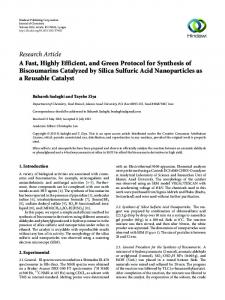
like BFB. Reference [3] also shows that the resulting estimators have the BRE property when the particular way in which individual failure transition probabilities are assigned is similar to that in BFB. Failure-distance biasing tries to exploit system structure in allocating probabilities to transitions, and [2], [105] apply similar ideas to BLR methods. In particular, they obtain additional efficiency gains by allocating probabilities to the individual failure transitions so that those failure transitions corresponding to component types that lie on minimum-cuts are more heavily weighted. Their algorithm does not need to maintain a list of all the minimum cuts; it needs only to maintain a list of all the time, components in a minimum cut. This can be done in where is the number of links. As with failure-distance biasing, one might not get any additional efficiency gains in certain systems that are unbalanced and/or have failure propagation. This is because in such systems the most likely paths to system failure might not lie along minimum cuts (the definition of minimum cut does not consider failure propagation). References [2], [3], [105] also describe improvements that are based on using semi-stationary cycles [106] rather than regenerative cycles. The simulation method is similar to the -cycle method [88] but the motivation for its use is different. In steadystate simulations of highly dependable systems, one usually uses the set of states with all components “up” as the regenerative state. However, when the BLR method is applied to systems with high degrees of redundancy, the regenerative cycles can become very long, leading to inefficient estimation. Thus, [2], [3], [105] instead consider a set of states with no 1-step transition probabilities within the set. An example is the set of states with failed components, where is less than the redundancy of the system (the least number of components that have to fail for the system to fail). The process in between two entrances to is a semi-stationary cycle, and has properties similar to regenerative cycles, except that these cycles are not necessarily -independent (thus complicating the construction of -confidence intervals). Also one needs to know the steady-state distribution at the times of entrances to this set, in on the set of states in order to apply IS; in general, this is very difficult to compute. These problems are similar to those in the -cycle method (see Section IV-B). 7) Other IS Methods: Another heuristic for failure biasing in acyclic models (of nonrepairable systems) is considered in [31], in which the extent to which one biases the failure transitions along a path leading to system failure is proportional to the path’s contribution to the measure being estimated. When applicable, this heuristic requires more overhead than simple failure biasing or BFB. Reference [66, ch. 10] describes some efficient simulation methods for -out-of- : G systems; these methods combine the IS technique known as forcing (see Section III-B) with some analytic calculations. 8) Some Empirical Results: Example #1 is a computing system (originally presented in [47] and then in many papers thereafter). Consider the unbalanced version of this computing system. Fig. 1 is the block diagram. It consists of • 2 sets of processors with 4 processors/set, • 2 sets of controllers with 2 controllers/set, • 6 clusters of discs, each consisting of 4 disk units.


Fig. 1. Computing-system example.

In a disk cluster, data are replicated so that one disk can fail without affecting the system. The “primary” data on a disk are replicated so that 1/3 is on each of the other 3 disks in the same cluster. Thus 1 disk in each cluster can be inaccessible without losing access to the data. It is assumed that when a processor of a given type fails it has a 0.01 probability of causing the operating processor of the other type to fail. Each unit in the system has 2 failure modes which occur with equal probability. The failure rates (per hour) are • 1/1000 for processors, • 1/20 000 for controllers, • 1/60 000 for disks. The repair rates (per hour) are • 1 for all mode 1 failures, • 1/2 for all mode 2 failures. This is an unbalanced system with a redundancy of 2. Components are repaired by a single RP who chooses a component at random from the set of failed units. The system is operational if all data are accessible to both processor types, which means that at least 1 processor of each type, 1 controller in each set, and 3 out of 4 disk units in each disk cluster are operational. Operational components continue to fail at given rates when the system is failed. To facilitate comparisons between simulation methods on the same CPU, simulation results (in the MSDIS framework) are quoted from the latest implementation of these methods [3]. BFB using a total of 200 000 cycles (100 000 cycles each for gave the the numerator and the denominator) and 3.8%, the steady-state unavailability estimate of 3.8% is the estimate of the RE corresponding to a 90% -confidence interval. The corresponding VRR was 167 with a TRR of 415. 6.5% with The BFB estimate of the MTTF was and . For the same problem, the most promising MSDIS implementation of the BLR method without the use of minimum cuts (denoted by BLBLR in [3]) gave • •

for the steady-state unavailability for the MTTF.


255

these cases because there were no system failure events with this method, even in the allotted run time of 10 events. The results suggest that for systems with appreciable redundancies, BFB is not at all effective, and the BLR method (with and without cuts) seems to improve the simulation efficiency. B. Transient Measures This section considers the estimation of transient measures in highly dependable Markov systems. Consider the three measures: unreliability: Fig. 2.

Network with redundancies.

-expected interval unavailability: Hence, for this example, without the use of additional information about the system, BFB does better than the BLR method. For the balanced version of this computing system (the results of which are in [3]), the improvements obtained by BFB and BLBLR are similar. The performance of the failure biasing method and BLR methods can be improved by using some information about component types on minimum cuts in the system. The most recommended MSDIS version of the BLR method with minimum cuts (denoted by BLBLRC in [3]) gave for the steady-state unavailability • for the MTTF. • There is appreciable improvement over BFB for the MTTF. For the balanced case of this network, there was appreciable improvement over BFB for both the MTTF and the unavailability. Consider the system (see Fig. 2) with important redundancies that was considered in [3]. The following description is from [3], with minor modification. The network contains 3 types of components: • Type A links contain 3 -identical components, which on average fail every 13(1/3) hours and can be repaired in half an hour. The type A link fails when 2 components are in the failed states. • Type B links contain 1 component, which on average fail every 40 hours and can be repaired in 1 hour. • Type C links contain 2 components, which on average fail every 26(1/3) hours and can be repaired in 2/3 hour. One component failure on a type C link causes the link to fail. The system operates as long as there exists a path along operating links between node 1 and node 20. There are 5 RP, and repairs make components “good as new.” Upon completing a repair, a RP selects (uniformly over the failed components in the network) the next component to repair. The results are , , for the BLBLR • , , for the BLBLRC • , , for BFB (worse than • ordinary simulation) in the estimation of the unavailability (estimates of which were of the order of 10 ). The BLBLRC methods when applied to another version of the same network yield orders of magnitude improvement over BFB when estimating unavailabilities that are of the order of 10 . No comparisons were made with ordinary simulation for

guaranteed availability:

Research in fast simulation for guaranteed availability is limited to experiments; see [47]. 1) Case 1: Small TH: Small TH means that the TH is small compared to the -expected lifetimes of components. From the analytic standpoint, it means that the TH is a constant, i.e., -independent of . The effectiveness of simulation techniques for small are studied again. For transient measures, failure biasing (relative to repair) alone might not be sufficient to observe many system failures, because it affects only the transitions of the embedded DTMC and not the random holding times in each state. To see why this is the case, note that the first component failure in a system occurs at a very low rate (the sum of failure rates of all the components). Thus, typically, the first component-failure occurs after time ; thus the chance that the system fails before the mission time expires is very small. To address this issue, “forcing” was introduced [71] to modify the random holding times in particular states. With forcing, the time to first component failure is sampled conditionally on the fact that it is less than , i.e., the time to first component failure is sampled from the distribution: for the transition rate out of state

(9)

under the original measure

. References [99], [115], [101] show that a “combination of BFB and forcing” gives BRE in estimating the unreliability and the -expected interval unavailability. From a modeling viewpoint, this implies that for small TH, the simulation can be very efficient. This agrees with experimental results [47], [99], [115], [101]. Another technique for estimating transient dependability measures is to combine failure biasing with “conditioning” [47]. Conditioning is applied by simulating the embedded DTMC until the system fails; failure biasing is used to generate the transitions. Random holding times are generated for each of the states visited, except for those states having slow transition rates (e.g., the “fully operational” state, which has no repairs taking place). Then for each generated sample path, one can analytically compute the conditional probability that

256


the system fails before time , given the path of the embedded DTMC and the sum of the holding times in the states that do not have slow transition rates. This computation involves calculating the convolution of exponentially distributed r.v., corresponding to the visits of the “conditioned out” states. The technique is guaranteed to reduce variance, but requires more computation. Experimental results and comparisons with the forcing technique, are in [47]. 2) Case 2: Moderate and Large TH: Even though, for small TH, the IS-based simulation of transient measures has the BRE property, it becomes inefficient for moderate and large TH. A moderate TH implies: is of the same order (of magnitude) as the -expected time to first component-failure. Any TH that is at least 1 order larger is termed “large.” For moderate TH, tuning the value of the failure biasing parameter through experimentation can yield efficient estimates [85], but it is difficult to provide guidelines for how should be set in general. For large TH, irrespective of the value of , the estimates using failure biasing are always poor, because the variance of the IS estimator increases with the variance of the likelihood ratio. The larger is, the more transitions there are in , and the variance of the likelihood ratio grows approximately exponentially with the number of transitions [39]. In estimating unavailability and MTTF, the expressions used in this paper are in terms of regenerative-cycle-based quantities, which are estimated using the regenerative method of simulation. Since in highly dependable systems, regenerative cycles typically contain a small number of transitions, the use of IS does not lead to a likelihood ratio with an important variance. A similar approach can be used in the context of transient measures. Though transient measures cannot be expressed exactly in terms of regenerative-cycle-based quantities, it is possible to develop bounds that are expressed in terms of regenerative-cycle-based quantities. Thus, when the direct application of IS to estimate the transient measure itself is inefficient, it is possible to estimate the bounds efficiently. For highly dependable systems these bounds are close to the transient measure in the sense explained in this section, [99], [115], [101], [102]. The is exponentially distributed with rate , which is equal to the sum of all component failure rates in state . From its . Let definition, • •

if the system does not fail in a regenerative cycle, time between the first system failure in a cycle and the end of the cycle if the system does fail: . Hence .

When the highly dependable system consists of highly reliable components, then most regenerative cycles consist of a single component failure transition followed by a component repair transition. Because component repair times are typically much smaller than component failure times, the regenerative cycle time consists mainly of the first component failure time, ( implies ), which is exponentially distributed with rate . The number of regenerative cycles until system failure is geometrically distributed with . The geometric sum (with acprobability ceptance probability ) of exponentially distributed r.v. (each of ). which has rate ) is exponentially distributed (with rate

Thus, is approximately exponentially distributed with rate . Let (10) then TH are modeled by to a small TH), then for large TH), as

it has been shown [101], [102] that , ( corresponds (corresponding to moderate and

and

thus we have an upper bound. Similarly, let

(11) then Also, as for

, for all . , as

i.e., the lower bound is close to the unreliability for moderate and large TH. and are in terms of regenerative-cycle-based Both and , use a MSDIS quantities. Hence for estimating is used to estimate the quantities type procedure in which and associated with rare events like and the original probability measure to estimate other quantities . like There are other bounds on the unreliability (in terms of regenerative-cycle-based quantities), like the ones in [11], [63]. These bounds are close for large , whereas the bounds in [101], [102] are close for both moderate and large . Bounds for the -expected interval unavailability were developed in [99], [115] and (as for the unreliability bounds) close to the actual measure for moderate and large . 3) Estimation of the Laplace Transform Function: An approach for estimating the actual transient measure (instead of estimating close bounds) for large TH is outlined in [13]. Instead of estimating the transient measure, the “Laplace transform function” of the transient measure is estimated (the transient measure is a function of ). Then a Laplace transform inversion method is used to estimate the transient measure for any given . The advantage of this approach is that the Laplace transform function of the transient measure can be expressed exactly in terms of Laplace transform functions of regenerative-cycle-based quantities, which can be estimated very efficiently using IS (if necessary).


For example, consider the unreliability. For any function the Laplace transform function is:

257

,

Let: and

One simulation-based approach for estimating derivatives is the likelihood-ratio derivative method [38], [93], which is now briefly described. Focus on estimating and its , only derivative with respect to . To estimate . requires simulating the embedded DTMC, and be the hitting time to and the cycle length of Let the embedded DTMC, respectively (the numbers of transitions until hitting and , respectively); then

Then the Laplace transform of the unreliability is [13]: The (original) transition-probability matrix of (under ) is . Then, under certain regularity conditions [38], [93],

(12) and are regenerative-cycle-based quantities. Both can be efficiently estimated using For any fixed , the can be efficiently estimated using ordinary IS, and the for some values simulation. Then, the method is: estimate and ], and then use a Laplace of [by estimating for a given . A transform inversion algorithm to obtain similar method for estimating the interval unavailability is in [13]. This transform approach [13] is a bit tedious to implement, but yields good experimental results. C. Estimation of Derivatives

The is determined within a single regenerative cycle. Thus, , generate regenerative cycles to estimate using the original measure , and collect observations: of The standard-simulation estimator of is

Performance measures of a system are (complicated) functions of the system parameters, such as the component failure and repair rates. Thus, one can compute derivatives of performance measures with respect to these parameters. This section reviews work in this area for highly dependable Markov systems. For example, determining the derivative of the MTTF with respect to a particular component’s failure rate. The derivative information is useful when designing systems, because this knowledge can help the designer identify system parts that need improvement. First consider estimating derivatives of the MTTF. Recall the ratio expression in (8) for the MTTF; then differentiate it with respect to some system parameter (e.g., some component’s failure rate).

(13) derivative operator with respect to . requires estimating each of these Thus, estimating 4 quantities in (13). A central limit theorem for the resulting esis derived in [83]; -confidence intervals timator of for the derivative can be formed. Section III-A discussed estiand ; thus the focus mating here is on estimating their derivatives.

Similarly, estimate in (13). One drawback of the likelihood-ratio derivative method is that it yields derivative estimators with large variances in many settings. Specifically, theoretical and empirical work, [36], [93], show that the variances of derivative estimators— • are typically much larger than those of the respective performance-measure estimators, • grow linearly in the -expected number of events in an observation. When regenerative simulation is used, an observation corresponds to a regenerative cycle, which typically consists of very few transitions for highly dependable Markov systems. Thus, the likelihood-ratio method seems to be well-suited for these types of systems. Theoretical studies in [77], [78] established that when estimating derivatives with respect to certain system parameters (e.g., failure rates of certain components) using ordinary simulation, the ratio of the RE of the estimate of and the estimate of remains bounded. This occurs when the parameter corresponds to one of the largest (in absolute value) sensitivities, where the sensitivity with respect to a parameter is defined as the product of and the derivative with respect to . Sensitivities measure how relative changes in a parameter value affect the overall performance. Thus, for parameters corresponding to the largest sensitivities, one can estimate the derivative with respect to and the performance mea-

258


sure with about the same relative accuracy. However, the RE of both these estimators go to infinity as the system unreliability tends to zero (see Section II-B); therefore IS must be used. The derivatives with respect to parameters that do not correspond to the largest sensitivities might not be estimated as efficiently as the performance measure when using ordinary simulation; [78] gives an example illustrating this. This section implements IS by simulating regenerative cycles using another probability measure and collecting observa, of tions , where is the likelihood ratio. the triplet is Then the IS estimator of

When BFB is applied, then the estimator of has BRE [78]. Necessary and sufficient conditions for BRE of derivative estimators obtained using other failure-biasing methods and more general IS schemes are established in [79], [81]. Reference [82] shows that even though the numerator in the MTTF ratio formula can be estimated with BRE using ordinary simulation, its derivative estimators can have unbounded RE. Consequently, if and its derivative are estimated using • ordinary simulation, • BFB is applied to the estimation of the denominator and its derivative, • all 4 terms are estimated mutually -independently (using measure-specific IS), then the resulting estimator of the derivative of the MTTF can have unbounded RE. On the other hand, if BFB is also used to , then its estimator has BRE and estimate so does the resulting estimator of the derivative of the MTTF. Experimental work in [83] seems to indicate that derivatives of the MTTF and the steady-state unavailability for large systems can be estimated efficiently using BFB. When estimating derivatives of the unreliability using BFB and forcing (see Section III-B), the empirical results show that the RE of the estimators are typically small when the TH is small, but they grow as the TH increases [101]. This is analogous to the behavior of (nonderivative) estimators of the unreliability, as discussed in Section III-B. Estimation of derivatives of the unreliability for large TH, using the bounding method in Section III-B, is treated in [101]. Reference [79] presents an example of a system showing and its derivatives using that when estimating simple failure biasing, estimators of derivatives with respect to certain component failure rates can have BRE, while the performance-measure estimator does not. Thus, it is possible to estimate a derivative more efficiently than the performance measure when using simple failure biasing. IV. FAST SIMULATION OF NON-MARKOV MODELS Notation NHPP intensity rate function of NHPP,

upper bound for intensity rate function time-homogeneous Poisson process with rate time of event of , Cdf, pdf of the lifetime of component , evaluated at hazard rate of the lifetime of component evaluated at hazard rate of the repair-time of component evaluated at , failure rate of component at time without, with IS , repair rate of component at time without, with IS , total failure rate of all components at time without, with IS , total repair rate of all components at time without, with IS , total event rate at time without, with IS , likelihood ratio of failure, repair events at time , likelihood ratio of pseudo, all events at time number of component failures by time det of operational components at time time component fails at its failure # length of a generic -cycle number of system failures in an -cycle in the steady-state DL total system failure time multiplied by the likelihood ratio on a generic (biased) -cycle -expectation under probability measure and initial distribution variance under probability measure and initial distribution number of batches used in the batch means method , generic batch mean of and its estimator , generic batch mean of DL and its estimator covariance under probability measures: for the first r.v., for the second r.v., and under initial distribution . This section uses IS to estimate dependability measures when the failure and repair times of components might not be exponentially distributed (under certain assumptions), and is based on [40], [54], [55], [87], [88]. Except for some technical and implementation details, most of the IS heuristics developed for Markov models also apply to non-Markov models. One approach to implement failure biasing (or forcing) in discrete-event systems is to reschedule failure events by sampling from new accelerated failure distributions [85].5 Heuristics and their implementation, as well as experimental results demonstrating the effectiveness of the techniques to estimate steady-state and transient measures are in [85], [86]. Another approach to IS in discrete-event systems (briefly described in this section) is based on the uniformization method of 5There

is considerable freedom in the choice of the new distributions.


simulation. The method requires the underlying (uniformized) distributions to have bounded hazard-rate functions. A closely related method which avoids generation of pseudo events is exponential transformation; here, the time to the next failure event is sampled directly from an exponential distribution [87]. Failure biasing or forcing are affected by increasing the failure rate (relative to the repair rate or the mission time, respectively). The latter two techniques are somewhat simpler to implement than the technique in [85], because failure events need not be rescheduled and are generated using only the exponential distribution. The next paragraph briefly describes the uniformization method of simulation, which is use in this section as a basis of our approach to IS in non-Markov models. Uniformization-Based Sampling: Uniformization (or thinning) is a simple technique for sampling (simulating) the event times of certain stochastic processes including NHPP, renewal processes, or Markov processes in continuous time on either discrete or continuous state spaces [22], [26], [49], [58], [72], with intensity function [104]. It is describe for a NHPP . Assume that for all for some finite can be sampled by constant . Then the event times of process as follows: thinning the , include (accept) as an event-time in For each with probability ; otherwise the point is not included (is rejected). Rejected events are sometimes called pseudo events. Throughout it is assumed that all rate functions are left-con; thus if an event occurs at some random tinuous: is the event rate just prior to time . time , then Renewal processes can be simulated using uniformization, is the hazard rate of the inter-event time disprovided that tribution at time . Uniformization can be generalized to cases in which the process being thinned is not a time-homogeneous , set Poisson process [72]. For example, at time , where has an exponential distribution with rate . The point is then accepted with probability . , for all . This requires only that Section IV-A describes how the uniformization method of simulation can be combined with IS to develop an effective technique for estimating transient measures in non-Markov models of highly dependable systems. A. Transient Measures Consider the problem of estimating the unreliability {time to system failure, for some fixed value of }. To simplify the notation, let there be 1 component of each type (although more general situations can be handled). The hazard rate [5] of component is then , which we assume is well defined and finite. , age of component at time . .] [If component is not operational at time then , elapsed repair time on component at time . [If component is not being repaired at time then . There are a variety of ways to use IS in simulations of such a system. Begin with a direct analog of forcing and BFB. This method is based on uniformization. If components are highly

259

reliable, then . If the failure and repair rates are bounded, then the system can be simulated (without IS) by uniformization as follows. , for all times ; Assume is a constant. Then a Poisson process with rate is simulated. Let an event in this Poisson process occur at time . That event is accepted as a component failure event with , and is accepted as a component repair probability . However, because it might be event with probability , another possibility exists: a pseudo-event (neither that a failure nor a repair occurs). This occurs with probability . The probability of a failure event is , and of a . repair event is whenFor highly reliable components, ever repairs are ongoing, thus the probability of a failure is very small. To accelerate failures, simply change the acceptance probabilities of the various event types, which is equivalent to changing component failure and repair rates to, say, [such that ], • [such that ]. • The likelihood ratio (at time ) is: (14) These likelihood ratios have a simple form. For example, let component fails on its own (not through failure propagation) times in .

(15)

Equation (15) assumes that the failure propagation probabilities are sampled from their given distributions. However, IS can also and can be applied to these as well. The terms be expressed similarly. The likelihood ratio can be computed (updated) recursively at uniformization event times during the simulation. The analog of BFB with forcing is accomplished as follows. If no repairs are ongoing (e.g., in the state where all compo, for some constant nents are operational), let . (In practice [87], could be chosen such that . This means that, with probability 0.8, some component fails before the TH expires.) If repairs are ongoing, : the total event rates the same as without IS. let , for some constant : given that the Then, let event is real, make it a failure event with probability . (In practice [87], is usually set in the range from 0.3 to 0.5.) Given a failure event, pick an operating component to fail with prob. Under appropriate technical conditions, it can ability be shown that such a heuristic for IS (which is the analog of forcing and failure biasing) results in estimates having BRE , and let there [55]. In particular, let exist a small positive parameter such that , where and . If IS is done such , [when ], that, for all

260

(when component is undergoing repair), then under some additional minor assumptions (including that the failure propagation probabilities are -indehave BRE as . pendent of ), the estimates of Because repair distributions might not have bounded hazard rates (e.g., discrete and uniform), it is desirable to seek effective IS methods that do not rely on uniformization for repair events. The above uniformization-based algorithm can be applied to just failure events: repair times are sampled directly from their original distributions, while uniformization is used to simulate failure events. The likelihood ratio is then : it does not include the repair event term . Again, under appropriate technical conditions, this modification results in BRE [55]. Uniformization can be computationally inefficient if there are many pseudo events. In addition, suppose events from a Poisson process with rate are accepted as failure events with probability . Then the time until an accepted event has an exponential distribution with rate . This suggests sampling the time to next failure event directly from an exponential distribution with rate . A generalization of this approach (exponential transformation) also results in estimates having BRE (under appropriate technical conditions [55]). The likelihood ratio takes on a somewhat different form [55], [87]. Empirical studies testing the competence of these methods are reported in [54], [55], [87]. Generally, good variance reducis small, say, less than 10 . The tion is obtained if are, the greater the can be made. smaller and Finally, though no formal study has been done, we anticipate that these techniques (with minor modifications) apply also for estimating the -expected interval unavailability. B. Steady-State Measures Non-Markov models of highly dependable systems might not possess an explicit regenerative structure. If they do not, then a ratio representation of steady-state measures in terms of regenerative-cycle-based quantities, such as in (5), is no longer possible. This section discusses an approach for the efficient estimation of steady-state measures, such as system unavailability and MTBF, in non-Markov nonregenerative models. The approach uses a representation of steady-state measures in terms of quantities based on -cycles: a sample path between two successive entries of the system into some set of states . In the context of highly dependable systems (as in Section II), choose to be the state in which all components are operational. Only when all component failure-time distributions are exponential (regardless of the repair-time distributions), entrance into the set constitutes a regeneration point, and a ratio representation of the steady-state unavailability, , in terms of regenerative-cycle-based quantities, as in (5), is still valid [85]. However, this is no longer true if component failure times are generally distributed. Therefore, in general, -cycles are not i.i.d., and one cannot use classical statistical techniques to estimate the variances of -cycle-based quantities. Instead, one can use the method of batch means to estimate the variances of these quantities by grouping successive -cycle-based quantities into nonoverlapping batches, and then treating the batch means as


i.i.d. observations; this is an approximation whose validity increases with the batch size. Let be the initial distribution of the corresponding (original) stochastic process upon entering the set , after the stochastic process has reached the steady-state. According to the definition of , is the steady-state joint distribution of the components’ ages upon entering the state in which all components are operational; upon entering , at least 1 component has an age 0. Under fairly general ergodicity conditions (which also ensure that the system returns to the set infinitely often), the ratio representation of in terms of -cycle-based quantities is:6 (16) the subscripts denote that the -expectation is with respect to the original probability measure (which governs the behavior of the original system) and the steady-state initial distribution of the -cycles. A ratio representation for the MTBF in terms of -cycle-based quantities is (17) The remainder of this section reviews the estimation of , which has been considered in [88]. A similar approach to estimate the MTBF is in [40]. Because system-failure is a rare event, ordinary simulation is ; this motivates the use of very inefficient to estimate IS. a new probability measure to simulate the system. a sample path in the original process, on which the . total system down-time is evaluated to be must satisfy the condition ,“ when. ever an -unbiased estimate of , With IS, likelihood ratio). ( should yield An appropriate choice of , which implies much better precision in estimating . can be estimated efficiently using ordinary simulation. Therefore, the ratio estimator in (16) can be written as (18) The resulting scheme is analogous to MSDIS for estimating the steady-state unavailability in Markov models [46] (see Section III-B). First, the system is simulated using the original for a sufficiently long time to approximately reach the steady-state. At that time, the initial distribution upon entry of -cycles is sufficiently close to , and begin to use the following splitting technique. For each (steady-state) -cycle, run the simulation (once or more) starting with the same component failure ages and using to get samples of and ; these are -biased -cycles. Then run the same -cycle using the to get a sample of 6For

details, see [10], [16], [27], [106].


261

; this is an original -cycle. This last run also ensures that the initial distribution, upon entering the next -cycle, is . Because successive -cycles are not -independent, use the method of batch means [68] to estimate variances and form -confidence intervals. After (approximately) reaching the steady-state, use and ; should be sufficiently large, so as to make the dependence between successive batch means -insignificant. (Experimental results in [88] indicate that in was used.) practice, need not be very large. In [88], It follows that the total number of original -cycles used in the . simulation is length of the original -cycle # , sample mean based on batch # :

An estimate of the steady-state unavailability is (22) From the CLT, for large

and ,

An estimate for the variance of is obtained from

of the estimate

(23) One could try to estimate fact that For sufficiently large , the s can be viewed as i.i.d. samples based on the batch of a generic r.v. . The estimate of . means method is is An estimate of

(19)

be the number of -biased cycles run for each origLet , because typically more cycles are inal cycle. Usually, than those required to estimate required to estimate to the same degree of RE. Thus the number of -biased -cycles in 1 batch is , and the total number of -biased -cycles used in the simulation is . , , be a sample of , evaluated Let at -biased -cycle # . , be the sample mean based on batch # : Let ,

For sufficiently large , the s can be viewed as i.i.d. samples is: of a generic r.v. . The respective estimate of

An estimate of

is

(20)

An estimate of

is

(21)

without using -cycles by using the

as with probability 1, where is the process representing the state-evolution of the system over time. One could then estimate using simulation as follows. Run a simulation of length , with large , and break-up the sample path into batches, each of size . To apply IS, one might have to use a change of measure for an entire batch. However, this would probably result in poor estimates because the batches would be large and the variance of the likelihood ratio grows approximately exponentially with the number of transitions [39]. Using -cycles avoids this problem by breaking the sample path into smaller pieces, and thus IS is typically applied for only a small number of events. A similar justification applies to the use of regenerative cycles when doing IS for Markov systems. This paper’s heuristic for IS is similar to that for regenerative non-Markov models [85]. In a biased -cycle, upon the occurrence of the first component failure, activate failure biasing to accelerate subsequent component failures relative to the ongoing repair. Failure biasing is continued until system failure or the end of the current -cycle. In BFB, various types of components have the same failure probability. As in Section IV-A, the uniformization method of simulation can be used to implement IS. In [40], [88], uniformization, combined with BFB, is used to estimate the steady-state unavailability and the MTBF, respectively. No proof is yet available to establish the BRE property of the resulting estimates. However, empirical results in [40], [88] seem to indicate the effectiveness of the approach in this section. Some experimental results from [88] are presented here. The system structure in this example is the same as described at the end of Section III-A except there are 2 processors in each set. However, the failure and repair behavior are appreciably different. Each component can now fail in only 1 failure mode. A preemptive resume-repair discipline is now assumed, with processors having the highest priority, and disks having the lowest priority. All repair time distributions are exponential with mean 1 hour. A failing processor in any of the 2 sets causes one processor in the other set to fail with probability 0.1. The mean

262


lifetimes for processors, controllers, and disks are assumed to be 20 k, 20 k, and 60 k hours, respectively. In [88], experimental results are presented for the Erlang, Weibull, exponential, and hyperexponential lifetime distributions. Results are presented here only for: all lifetimes have the Weibull distribution with shape parameter 1.25. For mean lifetimes of 20 k and 60 k hours, the scale parameters were 3.847 10 and 9.744 10 , respectively. The steady-state unavailability using IS was estimated to 9.18%. The RE corresponds to 99% -conbe 6.610 10 fidence. The estimate without IS was highly unstable and did not converge. All simulations were run for 64 k original -cyoriginal cycles per batch and biased cles with cycles for each original cycle. When the mean lifetimes were reduced by a factor of 10, the estimate of steady-state unavail9.87%. Even though the ability using IS was 6.856 10 steady-state unavailability estimate dropped by a factor of 100, the RE did not change appreciably, giving some validity to the BRE hypothesis.

V. CURRENT WORK AND FUTURE RESEARCH DIRECTIONS It is important to extend the applicability of IS to other classes of highly dependable systems. Reference [59] states that most of the failure biasing techniques mentioned in this paper break down when Assumption A (see Section III) does not hold. This can happen, for example, in systems with complicated repair policies like deferred and group repair. Two different approaches for the fast simulation of these models in the Markov setting have been presented in [60], [114], [61]. Extensions of these to non-Markov settings is an open-problem. Another area of research for non-Markov models is the development of techniques that handle systems with appreciable redundancies; the techniques in [2], [3], [105] apply mainly to Markov models. Also important from a practical viewpoint, is the development & extension of derivative estimation techniques [83] to • Markov models not satisfying Assumption A, • Markov models with appreciable redundancies, • non-Markov models. The robust implementation of fast simulation techniques in tools to evaluate highly dependable systems is the ultimate goal of this research and should be given an increasing attention. For related attempts, see [8], [47], [89], [90]. From a theoretical viewpoint, it is relevant to establish results pertaining to the effectiveness of IS techniques in Markov and non-Markov models, such as those in [3], [55], [60], [114], [61], [78], [79], [81], [98], [99], [115]. These results enhance our understanding of the capabilities and limitations of these techniques when used to estimate various measures in different classes of systems.

ACKNOWLEDGMENT The authors would like to thank a referee and C. Alexopoulos (the Special Section Editor) for their extremely careful reading of the paper and for providing helpful comments.

REFERENCES [1] A. A. Akyamac, Z. Haraszti, and J. K. Townsend, “Efficient simulation using DPR for multidimensional parameter spaces,” in Proc. 16th Int’l. Teletraffic Congress: Elsevier Science Publishers, 1999, pp. 767–776. [2] C. Alexopoulos and B. C. Shultes, “The balanced likelihood ratio method for estimating performance measures of highly reliable systems,” in Proc. 1998 Winter Simulation Conf.: IEEE Computer Society Press, 1998, pp. 1479–1486. , “Estimating reliability measures for highly-dependable Markov [3] systems using balanced likelihood ratios,” , 1999, to be published. [4] W. A. Al-Qaq, M. Devetsikiotis, and J. K. Townsend, “Importance sampling methodologies for simulation of communication systems with adaptive equalizers and time varying channels,” IEEE J. Selected Areas in Communications, vol. 11, pp. 317–327, 1993. [5] R. E. Barlow and F. Proschan, Statistical Theory of Reliability and Life Testing: Holt, Reinhart, Winston, 1981. [6] A. J. Bayes, “Statistical techniques for simulation models,” The Australian Computer J., vol. 2, pp. 180–184, 1970. , “A minimum variance sampling technique for simulation [7] models,” J. ACM, vol. 19, no. 4, pp. 734–741, 1972. [8] A. Blum, A. Goyal, and P. Heidelberger, “Modeling and analysis of system dependability using the system availability estimator,” in Digest of Papers: 24th Ann. Int’l. Symp. Fault Tolerant Computing: IEEE Computer Society Press, 1994, pp. 137–141. [9] A. Bobbio and K. S. Trivedi, “An aggregation technique for the transient analysis of stiff Markov chains,” IEEE Trans. Computers, vol. C-35, no. 9, pp. 803–814, 1986. [10] L. Breiman, Probability: Addison-Wesley, 1968. [11] M. Brown, “Error bounds for exponential approximations of geometric convolutions,” Annals of Probability, vol. 18, no. 3, pp. 1388–1402, 1990. [12] J. A. Carrasco, “Failure distance-based simulation of repairable fault-tolerant systems,” in Proc. 5th Int’l. Conf. Modeling Techniques and Tools for Computer Performance Evaluation, 1992, pp. 337–351. , “Efficient transient simulation of failure/repair Markovian [13] models,” in Proc. 10th Symp. Reliable and Distributed Computing, 1991, pp. 152–161. [14] G. Carter and E. J. Ignall, “Virtual measures: A variance reduction technique for simulation,” Management Science, vol. 21, no. 6, pp. 607–616, 1975. [15] C. S. Chang, P. Heidelberger, S. Juneja, and P. Shahabuddin, “Effective bandwidth and fast simulation of ATM in-tree networks,” Performance Evaluation, vol. 20, pp. 45–65, 1994. [16] R. Cogburn, “A uniform theory for sums of Markov chain transition probabilities,” Annals of Probability, vol. 3, pp. 191–214, 1975. [17] A. E. Conway and A. Goyal, “Monte Carlo simulation of computer system availability/reliability models,” in Proc. 17th Symp. on Fault-Tolerant Computing: IEEE Press, 1987, pp. 230–235. [18] M. Cottrell, J. C. Fort, and G. Malgouyres, “Large deviations and rare events in the study of stochastic algorithms,” IEEE Trans. Automatic Control, vol. AC-28, pp. 907–920, 1983. [19] P. J. Courtois, Decomposability: Queuing and Computer System Applications: Academic Press, 1977. [20] J. Couvillion, R. Freire, and R. Johnson et al., “Performability modeling using ULTRASAN,” IEEE Software, vol. 8, no. 5, pp. 69–80, 1991. [21] M. A. Crane and D. L. Iglehart, “Simulating stable stochastic systems, III: Regenerative processes and discrete-event simulations,” Operations Research, vol. 23, pp. 33–45, 1975. [22] N. M. van Dijk, “On a simple proof of uniformization for continuous and discrete-state continuous-time Markov chains,” Advances in Applied Probability, vol. 22, pp. 749–750, 1990. [23] N. M. van Dijk, B. R. Haverkort, and I. G. Niemegeers, Eds., “Performability modeling of computer and communication systems,” in Performance Evaluation, 1992, vol. 14, no. 3–4, appeared as special issue , pp. 135–275. [24] A. Dubi, A. Goldfeld, and K. Burn, “Algorithms for the calculation of the second moment of geometrical splitting in Monte Carlo,” Transport Theory and Statistical Physics, vol. 16, no. 8, pp. 1149–1165, 1987. [25] B. L. Fox and P. W. Glynn, “Discrete-time conversion for simulating semi-Markov processes,” Operations Research Letters, vol. 5, pp. 191–196, 1986. , “Discrete-time conversion for simulating finite-horizon Markov [26] processes,” SIAM J. Applied Mathematics, vol. 50, no. 5, pp. 1457–1473, 1990. [27] , “Estimating time averages via randomly-spaced observations,” Probability in Eng’g. & Informational Sciences, vol. 3, pp. 299–318, 1989.


[28] M. R. Frater, T. M. Lennon, and B. D. O. Anderson, “Optimally efficient estimation of the statistics of rare events in queuing networks,” IEEE Trans. Automatic Control, vol. 36, pp. 1395–1405, 1991. [29] M. J. J. Garvels and D. P. Kroese, “A comparison of RESTART implementations,” in Proc. 1998 Winter Simulation Conf.: IEEE Press, 1998, pp. 601–608. [30] R. M. Geist and K. S. Trivedi, “Ultra-high reliability prediction for fault-tolerant computer systems,” IEEE Trans. Computers, vol. C-32, pp. 1118–1127, 1983. [31] R. M. Geist and M. K. Smotherman, “Ultrahigh reliability estimates through simulation,” in Proc. Ann. Reliability & Maintainability Symp., 1989, pp. 350–355. [32] I. B. Gertsbakh, “Asymptotic methods in reliability theory: A review,” Advances in Applied Probability, vol. 16, pp. 147–175, 1984. [33] P. Glasserman, P. Heidelberger, P. Shahabuddin, and T. Zajic, “Splitting for rare event simulation: Analysis of simple cases,” in Proc. 1996 Winter Simulation Conf.: IEEE Computer Soc. Press, 1996, pp. 302–308. , “A large deviations perspective on the efficiency of multi[34] level splitting,” IEEE Trans. Automatic Control, vol. 43, no. 12, pp. 1666–1679, 1998. , “Multilevel splitting for estimating rare event probabilities,” Op[35] erations Research, vol. 47, no. 4, pp. 585–600, 1999. [36] P. W. Glynn, “Likelihood ratio gradient estimation: An overview,” in Proc, 1987 Winter Simulation Conf.: IEEE Press, 1987, pp. 366–375. , “A GSMP formalism for discrete event systems,” Proc. IEEE, vol. [37] 77, pp. 14–23, 1989. [38] , “Likelihood ratio derivative estimators for stochastic systems,” Communications of the ACM, vol. 33, pp. 75–84, 1990. [39] , “Importance sampling for Markov chains: Asymptotics for the variance,” Stochastic Models, vol. 10, pp. 701–717, 1995. [40] P. W. Glynn, P. Heidelberger, V. F. Nicola, and P. Shahabuddin, “Efficient estimation of the mean time between failures in nonregenerative dependability models,” in Proc. 1993 Winter Simulation Conf.: IEEE Press, 1993, pp. 311–316. [41] P. W. Glynn and D. L. Iglehart, “Importance sampling for stochastic simulations,” Management Science, vol. 35, pp. 1367–1392, 1989. [42] P. W. Glynn and W. Whitt, “The asymptotic efficiency of simulation estimators,” Operations Research, vol. 40, pp. 505–520, 1992. [43] C. Gorg and O. Fub, “Simulating rare event details of ATM delay time distributions with RESTART/LRE,” in Proc. 16th Int’l. Teletraffic Congress: Elsevier Science Pub., 1999, pp. 777–786. [44] A. Goyal, W. C. Carter, and E. de Souza e Silva, “The system availability estimator,” in Proc. 16th Symp. Fault-Tolerant Computing: IEEE Press, 1986, pp. 84–89. [45] A. Goyal and S. S. Lavenberg, “Modeling and analysis of computer system availability,” IBM J. Research and Development, vol. 31, no. 6, pp. 651–664, 1987. [46] A. Goyal, P. Heidelberger, and P. Shahabuddin, “Measure specific dynamic importance sampling for availability simulations,” in Proc. 1987 Winter Simulation Conf.: IEEE Press, 1987, pp. 351–357. [47] A. Goyal, P. Shahabuddin, and P. Heidelberger et al., “A unified framework for simulating Markovian models of highly reliable systems,” IEEE Trans. Computers, vol. C-41, pp. 36–51, 1992. [48] A. Goyal and A. Tantawi, “Evaluation of performability for degradable computer systems,” IEEE Trans. Computers, vol. C-36, no. 6, pp. 738–744, 1987. [49] D. Gross and D. R. Miller, “The randomization technique as a modeling tool and solution procedure for transient Markov processes,” Operations Research, vol. 32, no. 2, pp. 343–361, 1984. [50] P. J. Haas and G. S. Shedler, “Regenerative generalized semi-Markov processes,” Communications in Statistics—Stochastic Models, vol. 3, no. 3, pp. 409–438, 1987. [51] J. M. Hammersley and D. C Handscomb, Monte Carlo Methods: Methuen & Co., 1964. [52] Z. Haraszti and J. K. Townsend, “The theory of direct probability redistribution and its application to rare event simulation,” ACM Trans. Modeling and Computer Simulation, vol. 9, no. 2, pp. 105–140, 1999. [53] P. Heidelberger, “Fast simulation of rare events in queuing and reliability models,” ACM Trans. Modeling and Computer Simulation, vol. 5, no. 1, pp. 43–85, 1995. [54] P. Heidelberger, V. F. Nicola, and P. Shahabuddin, “Simultaneous and efficient simulation of highly dependable systems with different underlying distributions,” in Proc. 1992 Winter Simulation Conf.: IEEE Press, 1992, pp. 458–465.

263

[55] P. Heidelberger, P. Shahabuddin, and V. F. Nicola, “Bounded relative error in estimating transient measures in highly dependable non-Markovian systems,” ACM Trans. Modeling and Computer Simulation, vol. 4, pp. 137–164, 1994. [56] A. Hordijk, D. L. Iglehart, and R. Schassberger, “Discrete time methods for simulating continuous time Markov chains,” Advances in Applied Probability, vol. 8, pp. 772–788, 1976. [57] A. C. M. Hopmans and J. P. C. Kleijnen, “Importance sampling in system simulation: A practical failure,” Mathematics and Computing in Simulation XXI, pp. 209–220, 1979. [58] A. Jensen, “Markov chains as an aid in the study of Markov processes,” Skand. Aktuarietidskr, vol. 36, pp. 87–91, 1953. [59] S. Juneja and P. Shahabuddin, “Fast simulation of Markovian reliability/availability models with general repair policies,” in Proc. 22nd Symp. Fault-Tolerant Computing: IEEE Computer Soc. Press, 1992, pp. 150–159. , “Efficient simulation of Markov chains with small transition [60] probabilities,” in Research Report. New York: Dept. IEOR, Columbia Univ., 1997. , “A splitting based importance sampling algorithm for the fast [61] simulation of Markov chains with small transition probabilities,” in Research Report. New York: Dept. IEOR, Columbia Univ., 1998. [62] H. Kahn and T. E. Harris, “Estimation of particle transmission by random sampling,” US Nat’l. Bureau of Standards, Applied Mathematics Series, vol. 12, pp. 27–30, 1951. [63] V. V. Kalashnikov, “Analytic and simulation estimates of reliability for regenerative models,” in Systems Analysis, Modeling, Simulation. Berlin: Akademie Verlag, 1989, vol. 6, pp. 833–851. [64] J. Keilson, Markov Chain Models—Rarity and Exponentiality: SpringerVerlag, 1979. [65] L. C. Kioussis and D. R. Miller, “An importance sampling scheme for simulating the degradation and failure of complex systems during finite missions,” in Proc. 1983 Winter Simulation Conf.: IEEE Press, 1983, pp. 631–639. [66] I. N. Kovalenko, N. Yu. Kuznetsov, and P. A. Pegg, Mathematical Theory of Reliability of Time Dependent Systems With Practical Applications: Wiley, 1997. [67] D. P. Kroese and V. F. Nicola, “Efficient estimation of overflow probabilities in queues with breakdowns,” Performance Evaluation, vol. 36–37, pp. 471–484, 1999. [68] A. M. Law and W. D. Kelton, Simulation Modeling and Analysis, 3rd ed: McGraw-Hill, 2000. [69] D. Lieber, R. Y. Rubinstein, and D. Elmakis, “Quick estimation of rare events in stochastic networks,” IEEE Trans. Reliability, vol. 46, no. 2, pp. 254–265, June 1997. [70] D. Lieber, A. Nemirovskii, and R. Y. Rubinstein, “A fast Monte Carlo method for evaluating reliability indexes,” IEEE Trans. Reliability, vol. 48, no. 3, pp. 256–261, Sept. 1999. [71] E. E. Lewis and F. Bohm, “Monte Carlo simulation of Markov unreliability models,” Nuclear Eng’g. and Design, vol. 77, pp. 49–62, 1984. [72] P. A. W. Lewis and G. S. Shedler, “Simulation of nonhomogeneous Poisson processes by thinning,” Naval Research Logistics Quarterly, vol. 26, no. 3, pp. 403–413, 1979. [73] V. B. Melas, “Branching techniques for Markov-chain simulations (finite state case),” Statistics, vol. 25, pp. 159–171, 1994. [74] J. F. Meyer, “On evaluating the performability of degradable computing systems,” IEEE Trans. Computers, vol. C-39, no. 8, pp. 720–731, 1980. [75] A. P. A. van Moorsel, B. R. Haverkort, and I. G. Niemegeers, “Fault injection simulation: A variance reduction technique for systems with rare events,” in Dependable Computing for Critical Applications 2: SpringerVerlag, 1991, pp. 115–134. [76] R. R. Muntz, E. de Souza e Silva, and A. Goyal, “Bounding availability of repairable computer systems,” IEEE Trans. Computers, vol. C-38, no. 12, pp. 1714–1723, 1989. [77] M. K. Nakayama, “Simulation of highly reliable Markovian and nonMarkovian systems,” Ph.D. dissertation, Dep’t. Operations Research, Stanford University, California, 1991. , “Likelihood ratio derivative estimators in simulations of highly re[78] liable Markovian systems,” Management Science, vol. 41, pp. 524–554, 1995. [79] , “A characterization of the simple failure biasing method for simulations of highly reliable Markovian systems,” ACM Trans. Modeling and Computer Simulation, vol. 4, no. 1, pp. 52–88, 1994. [80] , “Fast simulation methods for highly dependable systems,” in Proc. 1994 Winter Simulation Conf.: IEEE Press, 1994, pp. 221–228.

264

[81] [82] [83] [84] [85]

[86] [87]

[88]

[89] [90] [91] [92] [93] [94] [95] [96] [97] [98] [99] [100] [101] [102] [103] [104] [105]

[106]


, “General conditions for bounded relative error in simulations of highly reliable Markovian systems,” Advances in Applied Probability, vol. 28, no. 3, pp. 687–727, 1996. , “On derivative estimation of the mean time to failure in simulations of highly reliable Markovian systems,” Operations Research, vol. 46, no. 2, pp. 285–290, 1998. M. K. Nakayama, A. Goyal, and P. W. Glynn, “Likelihood ratio sensitivity analysis for Markovian models of highly dependable systems,” Operations Research, vol. 42, no. 1, pp. 137–157, 1994. V. F. Nicola, “Lumping in Markov reward processes,” IBM, Yorktown Heights, IBM Research Report, RC 14 719, 1989. V. F. Nicola, M. K. Nakayama, P. Heidelberger, and A. Goyal, “Fast simulation of dependability models with general failure, repair and maintenance processes,” in Proc. 20th Int’l. Symp. Fault-Tolerant Computing: IEEE Computer Society Press, 1990, pp. 491–498. , “Fast simulation of highly dependable systems with general failure and repair processes,” IEEE Trans. Computers, vol. 42, no. 8, pp. 1440–1452, 1993. V. F. Nicola, P. Heidelberger, and P. Shahabuddin, “Uniformization and exponential transformation: Techniques for fast simulation of highly dependable non-Markovian systems,” in Proc. 22nd Int’l. Symp. Fault-Tolerant Computing: IEEE Computer Society Press, 1992, pp. 130–139. V. F. Nicola, P. Shahabuddin, P. Heidelberger, and P. W. Glynn, “Fast simulation of steady-state availability in non-Markovian highly dependable systems,” in Proc. 23rd Int’l. Symp. Fault-Tolerant Computing: IEEE Computer Society Press, 1993, pp. 38–47. W. D. Obal and W. H. Sanders, “An environment for importance sampling based on stochastic activity networks,” in Proc. 13th Symp. Reliable Distributed Systems: IEEE Press, 1994, pp. 64–73. , “Importance sampling simulation in ULTRASAN,” Simulation, vol. 62, no. 2, pp. 98–111, 1994. S. Parekh and J. Walrand, “A quick simulation method for excessive backlogs in networks of queues,” IEEE Trans. Automatic Control, vol. 34, no. 1, pp. 54–56, 1989. A. Reibman, K. S. Trivedi, S. Kumar, and G. Ciardo, “Analysis of stiff Markov chains,” ORSA J. Computing, vol. 1, no. 2, pp. 126–133, 1989. M. I. Reiman and A. Weiss, “Sensitivity analysis via likelihood ratios,” Operations Research, vol. 37, pp. 830–844, 1989. A. Rosenthal, “A computer scientist looks at reliability computations,” in Reliability and Fault Tree Analysis, R. Barlow, J. Fussell, and N. Singpurwalla, Eds: SIAM, 1975, pp. 133–152. G. Rubino, “Network reliability evaluation,” in State-of-the-Art in Performance Modeling and Simulation, K. Bagchi and J. Walrand, Eds: Gordon and Breach Books, 1996, pp. 275–302. J. S. Sadowsky, “Large deviations and efficient simulation of excessive backlogs in a GI/G/m queue,” IEEE Trans. Automatic Control, vol. 36, no. 12, pp. 1383–1394, 1991. P. Shahabuddin, “Simulation and analysis of highly reliable systems,” Ph.D. dissertation, Dep’t. of Operations Research, Stanford Univ., California, 1990. , “Importance sampling for the simulation of highly reliable Markovian systems,” Management Science, vol. 40, pp. 333–352, 1994. , “Fast transient simulation of Markovian models of highly dependable systems,” Performance Evaluation, vol. 20, pp. 267–286, 1994. , “Rare event simulation,” in Proc. 1995 Winter Simulation Conf.: IEEE Press, 1995, pp. 178–185. P. Shahabuddin and M. K. Nakayama, “Estimation of reliability and its derivatives for large time horizons in Markovian systems,” in Proc. 1993 Winter Simulation Conf.: IEEE Press, 1993, pp. 422–429. , “Fast simulation techniques for estimating the unreliability in large regenerative models of highly reliable systems,” in Research Report. New York: Columbia University, 1998. P. Shahabuddin, V. F. Nicola, and P. Heidelberger et al., “Variance reduction in mean time to failure simulations,” in Proc. 1988 Winter Simulation Conf.: IEEE Press, 1988, pp. 491–499. J. G. Shanthikumar, “Uniformization and hybrid simulation/analytic models of renewal processes,” Operations Research, vol. 34, no. 4, pp. 573–580, 1986. B. C. Shultes, “Regenerative techniques for estimating performance measures of highly dependable systems with repairs,” Ph.D. dissertation, School of Industrial & Systems Eng’g., Georgia Institute of Technology, Atlanta, 1997. R. F. Serfozo, “Semi-stationary processes,” Z. Wahrscheinlichkeitstheorie verw. Geb, vol. 23, pp. 125–132, 1972.

[107] D. Siegmund, “Importance sampling in the Monte Carlo study of sequential tests,” The Annals of Statistics, vol. 4, pp. 673–684, 1976. [108] A. D. Solovyev, “Asymptotic behavior of the time of first occurrence of a rare event,” Engineering Cybernetics, vol. 9, pp. 1038–1048, 1971. [109] S. G. Strickland, “Optimal importance sampling for quick simulation of highly reliable Markovian systems,” in 1993 Winter Simulation Conf. Proc.: IEEE Press, 1993, pp. 437–444. [110] M. Villen-Altamirano and J. Villen-Altamirano, “RESTART: A method for accelerating rare event simulation,” in Proc. 13th Int’l. Teletraffic Congress in Queuing Performance and Control in ATM, J. W. Cohen and C. D. Pack, Eds: Elsevier Science Publishers, 1991, pp. 71–76. [111] M. Villen-Altamirano, A. Martinez-Marron, J. Gamo, and F. Fernandez-Questa, “Enhancements of the accelerated simulation method RESTART by considering multiple thresholds,” in Proc. 14th Int’l. Teletraffic Congres in The Fundamental Role of Teletraffic in the Evolution of Telecommunication Networks, J. Labetoulle and J. W. Roberts, Eds: Elsevier Science Publishers, 1994, pp. 797–810. [112] M. Villen-Altamirano and J. Villen-Altamirano, “RESTART: A straightforward method for fast simulation of rare events,” in Proc. 1994 Winter Simulation Conf.: IEEE Press, 1994, pp. 282–289. [113] C. S. Chang, P. Heidelberger, S. Juneja, and P. Shahabuddin, “Effective bandwidth and fast simulation of ATM in-tree networks,” in Proc. Performance 1993 Conf. [114] S. Juneja and P. Shahabuddin, “Efficient simulation of Markov chains with small transition probabilities,” Management Science. [115] P. Shahabuddin, “Fast transient simulation of Markovian models of highly dependable systems,” in Proc. Performance 1993 Conf..

Victor F. Nicola has a Ph.D. in computer science from Duke University, North Carolina; a B.S. from Cairo University, Egypt; and M.S. in electrical engineering from Eindhoven University of Technology, The Netherlands. From 1979, he held faculty and research staff positions at Eindhoven University and at Duke University. In 1987, he joined IBM Thomas J. Watson Research Center, Yorktown Heights, as a Research Staff Member. Since 1993, he has been an Associate Professor at the Department of Electrical Engineering, University of Twente. His research interests include performance and reliability modeling, fault-tolerance, queuing theory, (rare event) simulation methodology, with applications to computer systems and telecommunication networks.

Perwez Shahabuddin is an Associate Professor of Industrial Engineering and Operations Research at Columbia University, New York. Prior to joining Columbia, he was a Research Staff Member at the IBM T.J. Watson Research Center. He received a Ph.D. (1990) in operations research from Stanford University. His research interests include stochastic modeling methods, and discrete event and Monte Carlo simulation methods, with application to performance modeling of computer systems, telecommunication networks, and financial systems. His research has been funded by the US National Science Foundation (NSF), AT&T, IBM, and AUM Systems. While at IBM, he was one of the developers of the System Availability Estimator (SAVE) modeling tool. Prof. Shahabuddin received the 1996 Outstanding Simulation Publication Award from INFORMS, a CAREER Award from the NSF in 1996, and a University Partnership Program Award from IBM in 1998. He received the Distinguished Faculty Teaching Award given by the Columbia Engineering School Alumni Association. He serves on the editorial board of Management Science, Stochastic Models, IIE Transactions Operations Engineering, IEEE TRANSACTIONS RELIABILITY, and ACM Transactions Modeling and Computer Simulation (Guest Editor).

Marvin K. Nakayama is an Associate Professor of Computer and Information Science at the New Jersey Institute of Technology. He has held positions at the IBM T.J. Watson Research Center, Rutgers School of Management, and the Columbia Business School. He received a Ph.D. (1991) in operations research from Stanford University. His research interests include simulation modeling and analysis, fault-tolerant systems, statistics, and applied probability. He received a CAREER Award from the US National Science Foundation, and is an Associate Editor for the ACM Transactions Modeling and Computer Simulation.

Techniques for fast simulation of models of highly

Techniques for fast simulation of models of highly

Suggest Documents

Techniques for fast simulation of models of highly ... - Semantic Scholar

optimizing single-pass simulation techniques for fast

Fast Simulation of Facilitated Spin Models

Automatic Generation of Fast Timed Simulation Models for ... - CiteSeerX

Fast simulation of highly dependable systems with general failure and ...

Modelling and simulation techniques for highly integrated ... - CiteSeerX

Model reduction techniques for fast blood flow simulation ... - CiteSeerX

Models and simulation techniques from stochastic geometry

FAST SIMULATION OF LARGE-SCALE GROWTH MODELS 1 ...

Fast Simulation of Fluid Models with Colored Jacobians - LinkÃ¶pings

Fast Simulation for the Performance Evaluation of

NEW TECHNIQUES FOR PARALLEL SIMULATION OF ... - CiteSeerX

Waveform Relaxation Techniques for Simulation of ... - doe.carleton.ca

SIMULATION MODELS FOR IMPLEMENTATION OF LEAN

Multilevel techniques for Reservoir Simulation

Deployment of Mathematical Simulation Models for ...

Advanced Simulation Techniques for Thick

DIAGNOSTIC TECHNIQUES FOR REGRESSION MODELS

Highly Efficient Techniques for Network Forensics

Analog Dithering Techniques for Highly Linear and

A Fast, Highly Efficient, and Green Protocol for Synthesis of ...

validation of simulation models - CiteSeerX

Simulation, Models, and Refactoring of

Calibration of Simulation Models