Temporal Query Answering in the Description ... - Semantic Scholar

Temporal Query Answering in the Description Logic DL-Lite ∗ Stefan Borgwardt, Marcel Lippmann, and Veronika Thost Theoretical Computer Science, TU Dresden, Germany {stefborg,lippmann,thost}@tcs.inf.tu-dresden.de

Abstract. Ontology-based data access (OBDA) generalizes query answering in relational databases. It allows to query a database by using the language of an ontology, abstracting from the actual relations of the database. For ontologies formulated in Description Logics of the DL-Lite family, OBDA can be realized by rewriting the query into a classical first-order query, e.g. an SQL query, by compiling the information of the ontology into the query. The query is then answered using classical database techniques. In this paper, we consider a temporal version of OBDA. We propose a temporal query language that combines a linear temporal logic with queries over DL-Lite core -ontologies. This language is well-suited to express temporal properties of dynamical systems and is useful in contextaware applications that need to detect specific situations. Using a firstorder rewriting approach, we transform our temporal queries into queries over a temporal database. We then present three approaches to answering the resulting queries, all having different advantages and drawbacks.

1

Introduction

Context-aware applications try to detect specific situations within a changing environment (e.g. a computer system or air traffic observed by radar) to be able to react accordingly. To gain information, the environment is observed by sensors (for a computer system, data about its resources is gathered by the operating system), and the results of sensing are stored in a database. A context-aware application then detects specific predefined situations based on this data (e.g. a high system load) and reacts accordingly (e.g. by increasing the CPU frequency). In a simple setting, such an application can be realized by using standard database techniques: the sensor information is stored in a database, and the situations to be recognized are specified as database queries [1]. In general, we cannot assume, however, that the sensors provide a complete description of the current state of the environment. For example, a sensor for certain information might not be available for a moment or not even exist. Thus, the closed world assumption employed by database systems (i.e. facts not present in the database are assumed to be false) is not appropriate since there may be facts of which it is unknown whether they hold or not. ∗

Partially supported by DFG SFB 912 (HAEC) and GRK 1763 (QuantLA).

In addition, though a complete specification of the environment usually does not exist, often some knowledge about its behavior is available. This knowledge can be used to formulate constraints on the interpretation of the predicates used in the queries, to detect more complex situations. In ontology-based data access (OBDA) [10], domain knowledge is encoded in ontologies using a Description Logic (DL). In this paper, we consider logics of the DL-Lite family, which are light-weight DLs with a low complexity for many reasoning problems [10]. This low complexity is due to the fact that reasoning problems in DL-Lite can often be reduced to answering a first-order query over a relational database. In order to recognize situations that evolve over time, we propose to add a temporal logical component to the queries. We use the operators of the temporal logic LTL, which allows to reason about a linear and discrete flow of time [20]. Usual temporal operators include next (#φ), which asserts that a property φ is true at the next point in time, eventually (3φ), which asks for φ to be satisfied at some point in the future, and always (2φ), which forces φ to be true at all time points in the future. We also use the corresponding past operators #− , 3− , and 2− . Consider, for example, a collection of servers providing several services. An important task is to migrate services between servers to balance the load. To decide when to migrate, we want to detect certain critical situations. We consider a process to be critical if it has an increasing workload, and at the same time the server it is running on is almost overloaded. Suppose that we want to detect those processes and servers that were in a critical situation at least twice within the past ten time units. This can be expressed by the query #−10 (3(Critical(x, y) ∧ #3Critical(x, y))), where Critical(x, y) := Server(x) ∧ Process(y) ∧ executes(x, y) ∧ Running(y) ∧ IncreasingWorkload(y) ∧ AlmostOverloaded(x). In this example, it is essential that future and past operators can be nested arbitrarily. One might argue that, as we are looking at the time line from the point of view of the current time point, and nothing is known about the future, it is sufficient to have only past operators. We will even show that in our setting it is indeed always possible to construct an equivalent query using only past operators. However, the resulting query is not very concise and it is not easy to see the situation that is to be recognized. Indeed, for propositional LTL eliminating the past operators from a query results in a blowup that is at least exponential and no constructions of size less than triply exponential are known [18]. Temporal extensions of DL-Lite [11] have been considered in the context of conceptual modeling [2,3,4], where the focus lies on checking concept satisfiability instead of query answering. Investigations of temporalized OBDA, the second major use case of DL-Lite, with temporal query answering as the most important reasoning problem [10], have started only quite recently. In [16], a framework is developed that combines conjunctive queries in an arbitrary DL and the temporal logic LTL. The algorithm for query answering in this setting is an LTL-satisfiability test using a sub-procedure to answer (atemporal) CQs.

In [6], a similar query language, a combination of LTL and CQs over the DL ALC, is proposed. In contrast to [16], its temporal component is allowed to influence the DL queries via the notion of rigid names, which are names whose interpretation does not change over time. The complexity increases depending on whether only rigid concept names or also rigid role names are allowed. Additionally, the latter paper also studies the so-called data complexity, where the complexity is measured only w.r.t. the size of the sensor data, i.e. the observations, but not w.r.t. the size of the query or the ontology. Another recent paper [5] examines temporal query answering in an extension of DL-Lite in which linear temporal operators are allowed to occur inside DL concepts, and proves first-order rewritability for query answering in this logic. In this paper, we follow an approach suggested in [16] to combine the firstorder rewriting techniques for atemporal query answering in logics of the DL-Lite family with a temporal component. The main idea is to use optimized database techniques to answer the actual queries. However, the existing techniques for answering temporal queries over temporal databases do not perfectly suit our purposes. In [14], the authors describe a temporal extension of the SQL query language that can answer temporal queries over a complete temporal database. However, in our setting the database containing all previous observations may grow huge very fast, but not all past observations are relevant for a particular query. In [13], an approach is described that reduces the amount of space needed; but the query language considered there allows only for past operators. In addition to describing how these approaches can be applied to our problem, we propose a new algorithm that extends the one from [13] and can also deal with future operators. All three approaches have different advantages and drawbacks. Additionally, we show how the new algorithm can be extended to deal with rigid concept names for a specific subclass of queries. Unfortunately, there seems to be no simple way to adapt the algorithm to deal with rigid role names. This paper is an extension of the recently appeared workshop paper [8]. The formal proofs of our results can be found in the technical report [9].

2

Preliminaries

We first describe the DL component, and then the temporal component of our query language. The DL-Lite family consists of various DLs that are tailored towards conceptual modeling and allow to realize query answering using classical database techniques. We only consider DL-Lite core as a prototypical example. Definition 1. Let NC , NR , and NI be non-empty, pairwise disjoint sets of concept, role, and individual names, respectively. A role expression is either a role name P1 ∈ NR or an inverse role P2− with P2 ∈ NR . A basic concept is of the form A or ∃R, where A ∈ NC and R is a role expression. A general concept is of the form B or ¬B, where B is a basic concept. A concept inclusion is of the form B v C, where B is a basic concept and C is a general concept. An assertion is of the form A(a) or P (a, b), where A ∈ NC ,

P ∈ NR , and a, b ∈ NI . A TBox (or ontology) is a finite set of concept inclusions, and an ABox is finite set of assertions. The semantics of DL-Lite core is defined through the notion of an interpretation. Definition 2. An interpretation is a pair I = (∆I , ·I ), where ∆I is a nonempty set (called domain) and ·I is a function that assigns to every A ∈ NC a set AI ⊆ ∆I , to every P ∈ NR a binary relation P I ⊆ ∆I × ∆I , and to every a ∈ NI an element aI ∈ ∆I . This function is extended to role expressions, basic concepts, and general concepts as follows: (P − )I := {(e, d) | (d, e) ∈ P I }, (∃R)I := {d | there is an e ∈ ∆I such that (d, e) ∈ RI }, and (¬C)I := ∆I \ C I . I is a model of B v C if B I ⊆ C I , of A(a) if aI ∈ AI , and of P (a, b) if I I (a , b ) ∈ P I . We write I |= T if I is a model of all concept inclusions in the TBox T , and I |= A if I is a model of all assertions in the ABox A. An ABox A is consistent (w.r.t. a TBox T ) if there is an I with I |= A and I |= T . We assume that all interpretations I satisfy the unique name assumption (UNA), i.e. for all a, b ∈ NI with a 6= b, we have aI 6= bI . We now introduce the notion of temporal knowledge bases. Intuitively, they contain sensor data (ABoxes) for all previous time points, and a global TBox. Definition 3. A temporal knowledge base (TKB) K = h(Ai )0≤i≤n , T i consists of a finite sequence of ABoxes Ai and a TBox T , where the ABoxes Ai can only contain concept names that also occur in T . Let I = (Ii )0≤i≤n be a sequence of interpretations Ii = (∆, ·Ii ) over a fixed non-empty domain ∆. Then I is a model of K (written I |= K) if Ii |= Ai and Ii |= T for all i, 0 ≤ i ≤ n. Similar to what was done in [6,16], our temporal query language is based on conjunctive queries [1,12]. The main difference is that we do not allow for negation, as in DL-Lite arbitrary negation is disallowed. In contrast to [5], we also do not allow temporal operators inside concepts. These restrictions allow us to apply first-order rewritability of (atemporal) conjunctive queries in a black-box fashion to obtain a similar result for our temporal query language (see Section 3). Definition 4. Let NV be a set of variables. A conjunctive query (CQ) is of the form φ = ∃y1 , . . . , ym .ψ, where y1 , . . . , ym ∈ NV and ψ is a (possibly empty) finite conjunction of atoms of the form A(z) for A ∈ NC and z ∈ NV ∪ NI ( concept atom); or r(z1 , z2 ) for r ∈ NR and z1 , z2 ∈ NV ∪ NI ( role atom). The empty conjunction is denoted by true. Temporal conjunctive queries (TCQs) are built from CQs as follows: each CQ is a TCQ, and if φ1 and φ2 are TCQs, then so are φ1 ∧ φ2 (conjunction), φ1 ∨ φ2 (disjunction), #φ1 (strong next), φ1 (weak next), #− φ1 (strong previous), − φ1 (weak previous), φ1 U φ2 (until), and φ1 S φ2 (since).

•

•

•

•

The symbols #− , − , and S are called past operators, the symbols #, , and U are future operators. All results also hold in the presence of the additional temporal operators 2 (always), 2− (always in the past), 3 (eventually), and 3− (some time in the past) [9], but we omit them here for space reasons.

We denote the set of individuals occurring in a TCQ φ by Ind(φ), the set of variables occurring in φ by Var(φ), the set of free variables in φ by FVar(φ), and the set of atoms occurring in φ by At(φ). A TCQ φ is called Boolean if FVar(φ) = ∅. We further denote by Sub(φ) the set of all TCQs occurring as subqueries in φ (including φ itself). A union of conjunctive queries (UCQ) is a disjunction of CQs. For our purposes, it is sufficient to define the semantics for Boolean CQs and TCQs. As usual, it is given using the notion of a homomorphism [12]. Definition 5. Let I = (∆, ·I ) be an interpretation and ψ be a Boolean CQ. A mapping π : Var(ψ) ∪ NI → ∆ is a homomorphism of ψ into I if π(a) = aI for all a ∈ NI , π(z) ∈ AI for all concept atoms A(z) in ψ, and (π(z1 ), π(z2 )) ∈ rI for all role atoms r(z1 , z2 ) in ψ. We say that I is a model of ψ (written I |= ψ) if there is such a homomorphism. Let now φ be a Boolean TCQ. For a sequence of interpretations I = (Ii )0≤i≤n and i with 0 ≤ i ≤ n, we define I, i |= φ by induction on the structure of φ: I, i |= ∃y1 , . . . , ym .ψ I, i |= φ1 ∧ φ2 I, i |= φ1 ∨ φ2 I, i |= #φ1 I, i |= φ1 I, i |= #− φ1 I, i |= − φ1 I, i |= φ1 U φ2

• •

I, i |= φ1 S φ2

iff Ii |= ∃y1 , . . . , ym .ψ iff I, i |= φ1 and I, i |= φ2 iff I, i |= φ1 or I, i |= φ2 iff i < n and I, i + 1 |= φ1 iff i < n implies I, i + 1 |= φ1 iff i > 0 and I, i − 1 |= φ1 iff i > 0 implies I, i − 1 |= φ1 iff there is some k, i ≤ k ≤ n such that I, k |= φ2 and I, j |= φ1 for all j, i ≤ j < k iff there is some k, 0 ≤ k ≤ i such that I, k |= φ2 and I, j |= φ1 for all j, k < j ≤ i.

Here we assume that there is no time point before 0 or after n, similar to the temporal semantics used for LTL in [23] or for temporal query languages for databases [13,17,21]. As in classical LTL, one can show that φ1 S φ2 is equivalent to φ2 ∨ (φ1 ∧ #− (φ1 S φ2 )), and a similar equivalence holds for U. We are now ready to introduce the central reasoning problem of this paper, namely to find certain answers to TCQs. Definition 6. Let φ be a TCQ, I = (Ii )0≤i≤n a sequence of interpretations, and i ≥ 0. The mapping a : FVar(φ) → NI is an answer to φ w.r.t. I at time point i if I, i |= a(φ), where a(φ) denotes the Boolean TCQ that is obtained from φ by replacing the free variables according to a. Let further K = h(Ai )0≤i≤n , T i be a TKB. A mapping a : FVar(φ) → NI is a certain answer to φ w.r.t. K at time point i if for every J |= K, we have J, i |= a(φ). The set of all answers to φ w.r.t. I at time point i is denoted by Ans(φ, I, i), and the set of all certain answers to φ w.r.t. K is denoted by Cert(φ, K, i). Recall that our main interest lies in finding answers to queries at the current time point, i.e. computing the sets Ans(φ, I) := Ans(φ, I, n) or Cert(φ, K) := Cert(φ, K, n). We will sometimes use the abbreviation false := A(x) ∧ A0 (x), where A, A0 are new concept names for which we assume that the concept inclusion A v ¬A0 is contained in the global TBox T .

3

Answering Temporal Conjunctive Queries

For computing the set of certain answers for a conjunctive query, the rewriting approach [10] can be employed. It compiles the information contained in the TBox into the query and evaluates the query w.r.t. the ABox (viewed as database) using classical database techniques. A similar approach is possible for TCQs. Definition 7. For an ABox A, the interpretation DB(A) := (NI , ·DB(A) ) is defined as follows: – aDB(A) := a for all a ∈ NI ; – ADB(A) := {a | A(a) ∈ A} for all A ∈ NC ; and – P DB(A) := {(a, b) | P (a, b) ∈ A} for all P ∈ NR . As shown in [10], this interpretation is the smallest model of A. In order to employ database techniques, we must assume DB(A), and thus NI , to be finite. Proposition 8 ([10]). Let ψ be a CQ, A be an ABox, and T be a TBox. There is a canonical model IA,T of A and T and a UCQ ψ T such that Cert(ψ, hA, T i) = Ans(ψ, IA,T ) = Ans(ψ T , DB(A)). We now use this proposition to show a similar result for TCQs. Let φ be a TCQ and K = h(Ai )0≤i≤n , T i be a TKB. The TCQ φT is obtained by replacing each CQ ψ occurring in φ by ψ T . Note that φT is again a TCQ since ψ T is always a UCQ. Let furthermore IK := (IAi ,T )0≤i≤n and DB(K) := (DB(Ai ))0≤i≤n . The following theorem can be shown by a straightforward induction on the structure of φ. Theorem 9. For every TCQ φ, TKB K = h(Ai )0≤i≤n , T i, and i ≥ 0, we have Cert(φ, K, i) = Ans(φ, IK , i) = Ans(φT , DB(K), i). More importantly, for every TCQ φ and TKB K = h(Ai )0≤i≤n , T i, it holds that Cert(φ, K) = Ans(φT , DB(K)). It thus remains to show how to compute the set Ans(φ, I) for a TCQ φ and a sequence I = (Ii )0≤i≤n of interpretations over a finite domain. A first possibility is to view I as a temporal database and rewrite φ into an ATSQL query [14]. However, since our goal is to monitor processes that produce new data in very short time intervals, storing all the data for all previous time points is not feasible. Therefore, we describe two different approaches that reduce the amount of space necessary to compute Ans(φ, I). Since we are interested in the answers at the last time point, the idea is to keep only the past information necessary to answer the query φ. In the first approach (Section 4), we rewrite φ into a TCQ φ0 without future operators, employing a construction described in [15]. We then compute Ans(φ0 , I) using an algorithm described in [13,22] that uses a so-called bounded history encoding, which means that the space required by the algorithm is constant w.r.t. the number n of previous time points. Only the current state of the database and some auxiliary relations have to be stored.

In Section 5, we generalize the algorithm from [13] to directly deal with the future operators. The main difference is that we do not consider negation or arbitrary first-order queries. Unfortunately, the space required by this algorithm is in general exponential in n and thus does not constitute a bounded history encoding in the sense of [13,22]. However, it allows us to circumvent the nonelementary blow-up of the formula resulting from the reduction in [15].

4

Eliminating Future Operators

To rewrite a TCQ φ into an equivalent TCQ that does not contain future operators, we employ the separation theorem for propositional LTL [15]. We describe here only the general idea, details can be found in the technical report [9]. The separation theorem cannot be applied directly since our temporal semantics differs from that in [15]: the only temporal operators in [15] are strict versions of U and S, and the semantics is defined w.r.t. bounded past and unbounded future. To apply this theorem, we replace the CQs in φ by propositional variables, rewrite U and S into their restrict counterparts, and use an additional propositional variable to delimit the time interval from 0 to n. b We can then apply the separation theorem to the resulting LTL-formula φ. 0 b We obtain an equivalent LTL-formula φ with negation which is a Boolean combination of temporal subformulae that either contain only strict S operators or only strict U operators. In this construction, subformulae of φb are copied and rearranged, but no additional propositional variables are introduced. Since we are interested in evaluating φ at n, we can replace all variables in φb0 that are in the scope of a strict U by false. The reason for this is that such variables are only evaluated at time points after n, where all variables are false. The resulting formula is then simplified to eliminate all strict U operators, and then translated back into a Boolean TCQ φ0 by replacing the propositional variables by the corresponding CQs. Note that φ0 contains no future operators. We then apply the algorithm described in [13] to iteratively compute the answers to φ0 at each time point.1 The main advantage of this approach is that we can compute this set iteratively and such that the required memory is independent of the length of the sequence I. More formally, let I = (Ii )i≥0 be an infinite sequence of interpretations representing the observations over all time points. In our setting, these interpretations are generated from an infinite sequence of ABoxes that represent the observed sensor data using the construction of Section 3. At each time point i ≥ 0, we only have access to the finite prefix I(i) := (Ij )0≤j≤i of I of length i + 1. Let ∆ be the shared domain of the interpretations in I. The algorithm from [13] works on φ0 as follows. On input I0 , it computes a first-order interpretation I00 of several auxiliary predicates. Intuitively, for each subformula ψ of φ0 beginning with a past operator, the algorithm stores the I0 answers Ans(ψ, I(0) ) ⊆ ∆FVar(ψ) for ψ in a new relation Aψ0 of arity |FVar(ψ)|. 1

Before we can use the algorithm presented in [13], we need another rewriting step since in that paper the semantics of S is slightly different (see [9] for details).

The set Ans(φ0 , I(0) ) can then easily be computed from I0 and I00 . Afterwards, the algorithm disregards I0 and keeps only the information computed in I00 . On input I1 , it then updates I00 to a new interpretation I10 , which allows it to compute Ans(φ0 , I(1) ), and so on. The memory requirements of this algorithm are bounded polynomially in the size of ∆, in the number of concept and role names, and in the number of past operators occurring in φ0 , and exponentially in the number of free variables occurring below past operators. However, the memory requirements do not depend on the length of the sequence of interpretations seen so far. This is called a bounded history encoding in [13]. Overall, the presented approach has, however, several drawbacks. First, the rewritings from φ to φb and from φb0 to φ0 may duplicate subformulae, which can cause exponential blowups in the size of φ. This could be avoided by applying a reduction similar to the one for propositional LTL in [15] directly to φ. However, since the reduction in [15] is already non-elementary in the size of the formula, this is not much more efficient. Hence, the presented approach is best suited for answering simple, small queries φ over large databases.

5

A New Algorithm

In this section, we present an algorithm that computes the set Ans(φ, I) without the need to eliminate the future operators beforehand, thereby avoiding the non-elementary blowup of the construction described in the previous section. However, the memory requirements of this new algorithm are not independent of the number of previous time points. From now on, let φ be a fixed TCQ and I = (Ii )i≥0 be a fixed infinite sequence of interpretations over the same finite domain ∆. For i ≥ 0, we denote by I(i) := (Ij )0≤j≤i the finite prefix of I of length i + 1. Our algorithm iteratively computes the sets Ans(φ, I(i) ). It uses as data structure so-called answer formulae, which represent TCQs in which some parts have already been evaluated. In particular, they do not contain CQs any more, but sets of already computed answers to subqueries. Additionally, they may contain variables (different from those in NV ) that serve as place-holders for subqueries that have to be evaluated at the next time point. For ease of presentation, we assume in the following that NV is finite and that answers are of the form a : NV → ∆ instead of a : FVar(φ) → ∆. Thus, when we talk about answers, we mean mappings a : NV → ∆, and in particular Ans(. . .) refers to a set of such mappings, i.e. a subset of ∆NV .2 Definition 10. Let FSub(φ) denote the set of all subqueries of φ of the form #ψ1 , ψ1 , or ψ1 U ψ2 . For j ≥ 0, we denote by Varφj the set of all variables of i the form xψ j for ψ ∈ FSub(φ). The set AFφ of all answer formulae for φ at i ≥ 0 is the smallest set satisfying the following conditions:

•

2

In an implementation, one should restrict the intermediate computations of answers for subqueries ψ to FVar(ψ). But then one has to be more careful when combining answers to different subqueries.

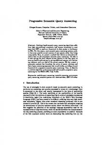
Table 1. Computing answer formulae for a TCQ φ

Φ0 (φ)

Φ0i (φ)

CQ ψ1 ψ1 ∧ ψ2 ψ1 ∨ ψ2 #ψ1 #− ψ1 ψ1 − ψ1 ψ1 U ψ2 ψ1 S ψ 2

Ans(ψ1 , I(0) ) Φ0 (ψ1 ) ∩ Φ0 (ψ2 ) Φ0 (ψ1 ) ∪ Φ0 (ψ2 ) 1 x#ψ 0 ∅ ψ x0• 1 NV ∆ 1 U ψ2 Φ0 (ψ2 ) ∪ (Φ0 (ψ1 ) ∩ xψ ) 0 Φ0 (ψ2 )

Ans(ψ1 , I(i) ) Φ0i (ψ1 ) ∩ Φ0i (ψ2 ) Φ0i (ψ1 ) ∪ Φ0i (ψ2 ) 1 x#ψ i Φi−1 (ψ1 ) ψ xi• 1 Φi−1 (ψ1 ) 1 U ψ2 Φ0 (ψ2 ) ∪ (Φ0i (ψ1 ) ∩ xψ ) i Φ0i (ψ2 ) ∪ (Φ0i (ψ1 ) ∩ Φi−1 (ψ1 S ψ2 ))

• •

– Every set A ⊆ ∆NV is an answer formula for φ at i. φ – Every xψ j ∈ Varj with j ≤ i is an answer formula for φ at i. – If α1 and α2 are answer formulae for φ at i, then so are α1 ∩ α2 and α1 ∪ α2 . In order to evaluate these answer formulae, we introduce the notion of correctness. Intuitively, an answer formula α for φ at i is correct for i if we obtain the set Ans(φ, I(i) ) by replacing the variables xψ j in α by appropriate sets of answers and evaluating ∩ and ∪ as set intersection and union, respectively. N

Definition 11. We define the function evaln : AFnφ → 2∆ V , n ≥ 0, as follows: – evaln (A) := A if A ⊆ ∆NV ;  Ans(ψ1 , I(n) , j + 1) if j < n   Ans(ψ, I(n) , j + 1) if j < n n ψ – eval (xj ) :=  ∅ if j = n    NV ∆ if j = n – evaln (α1 ∩ α2 ) := evaln (α1 ) ∩ evaln (α2 ); and – evaln (α1 ∪ α2 ) := evaln (α1 ) ∪ evaln (α2 ).

and and and and

ψ ψ ψ ψ

•

= #ψ1 or ψ = ψ1 ; = ψ1 U ψ2 ; = #ψ1 or ψ = ψ1 U ψ2 ; = ψ1 ;

•

We say that a mapping Φ : Sub(φ) → AFiφ is correct for i ≥ 0 if for all n ≥ i and for all ψ ∈ Sub(φ), we have evaln (Φ(ψ)) = Ans(ψ, I(n) , i). In particular, if Φ : Sub(φ) → AFiφ is correct for i, then evali (Φ(φ)) = Ans(φ, I(i) ), 1 U ψ2 which is the set we want to compute. Note that xψ is actually a placej holder for #(ψ1 U ψ2 ) since we evaluate the U operator according to the recursive equivalence ψ1 U ψ2 ≡ ψ2 ∨ (ψ1 ∧ #(ψ1 U ψ2 )) (cf. Table 1). The algorithm works as follows. It first computes a mapping Φ0 that is correct for 0, which is used to compute the next mapping Φ1 when the interpretation I1 becomes available. This mapping is correct for 1 and can be used to compute the next mapping Φ2 , and so on. In each step, to compute Φi+1 , we only need Φi and the interpretation Ii+1 . We recursively define the mapping Φ0 : Sub(φ) → AF0φ as shown in the second column of Table 1. Here, CQs are answered, e.g. by evaluating them as first-order queries over the database I0 [1].

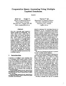
Table 2. An example computation φ

ψ1 1 xψ 0 NV

Φ0 (φ) Ans(φ, I(0) ) ∆

ψ2 B0 ∪ (A0 ∩ B0

ψ1 S ψ2 2 xψ 0 )

2 B0 ∪ (A0 ∩ xψ 0 ) B0

ψ1 ψ2 0 1 2 xψ B1 ∪ (A1 ∩ xψ 1 1 ) Φ1 (ψ2 ) ∪ (x1 ∩ (B0 ∪ (A0 ∩ x0 ))) ψ1 ψ2 ψ1 x1 B1 ∪ (A1 ∩ x1 ) Φ1 (ψ2 ) ∪ (x1 ∩ (B0 ∪ (A0 ∩ Φ1 (ψ2 )))) ψ2 1 ≡ ((xψ 1 ∩ B0 ) ∪ B1 ) ∪ (A1 ∩ x1 ) (1) NV Ans(φ, I ) ∆ B1 B0 ∪ B1

Φ01 (φ) Φ1 (φ)

ψ1 ψ1 ψ2 1 2 xψ B2 ∪ (A2 ∩ xψ 2 2 ) Φ2 (ψ2 ) ∪ (x2 ∩ (((x1 ∩ B0 ) ∪ B1 ) ∪ (A1 ∩ x1 ))) ψ1 ψ2 ≡ ((x2 ∩ ((C1 ∩ B0 ) ∪ B1 )) ∪ B2 ) ∪ (A1 ∩ x2 ) Ans(φ, I(2) ) ∆NV B2 (C1 ∩ B0 ) ∪ B1 ∪ B2

Φ2 (φ)

Assume now that Φi−1 : Sub(φ) → AFφi−1 is a function containing only variables with index i − 1. We proceed as follows to construct a new function that contains only variables with index i. We recursively define the mapping Φ0i : Sub(φ) → AFiφ similarly to Φ0 as given in the third column of Table 1. Example 12. Consider the TCQ ψ1 S ψ2 with two subqueries referring to the future, ψ1 := C(x) and ψ2 := A(x) U B(x), and let A0 := Ans(A(x), I(0) ), and similarly for the other CQs and time points. The answer formulae Φ0 and Φ01 are listed in Table 2.

•

The difference to the definition of Φ0 is that the answer formulae for past operators are computed using the answer formulae for the previous time point. This means that Φ0i may still contain variables with index i − 1. We now remove these old variables by substituting them appropriately. For example, since x#ψ i−1 is a place-holder for the answers to ψ w.r.t. I(n) at i, we can now replace it by Φ0i (ψ). However, this formula may itself contain another old variable, and thus we have to be careful about the order in which we do these substitutions. Since each Φ0i (ψ) can contain only variables that refer to subqueries of ψ, by replacing the variables for “smaller” subqueries first, we ensure that all variables with index i − 1 are eliminated. The details of this construction can be found in [9]. We obtain a mapping Φi : Sub(φ) → AFiφ that is correct for i. Lemma 13. For each i ≥ 0, the mapping Φi is correct for i. Example 14. Consider again the query ψ1 S ψ2 from Example 12. Since Φ01 (ψ1 ) and Φ01 (ψ2 ) do not contain variables with index 0, the value of Φ1 is the same 2 as that of Φ01 for both of these subqueries. We only have to replace xψ 0 within 0 Φ1 (ψ1 S ψ2 ) by Φ1 (ψ2 ) to obtain Φ1 (ψ1 S ψ2 ) as listed in Table 2. To obtain the answers at time point 1, we can now replace the remaining variables in according to eval1 , which yields Ans(ψ1 S ψ2 , I(1) ) = B0 ∪ B1 . Consider now the algorithm, which, on input φ and I, computes the mappings Φi as described above, and outputs evali (Φi (φ)) for each i ≥ 0. The following is a trivial consequence of the correctness of these mappings.

Theorem 15. Given a TCQ φ and an infinite sequence I = (Ii )i≥0 of interpretations, the algorithm outputs Ans(φ, I(i) ) for each i ≥ 0. It is easy to compute the sets evali (Φi (φ)) = Ans(φ, I(i) ) for i ≥ 0 since each NV (see of the variables xψ i in Φi (φ) simply has to be replaced by either ∅ or ∆ Definition 11). However, as mentioned earlier, the size of the formula Φi (φ) may depend exponentially on the length i of the current sequence of interpretations. Example 16. Consider again the query ψ1 S ψ2 from Example 12. After replac2 2 ing xψ by Φ1 (ψ2 ), the variable xψ occurs twice in Φ1 (ψ1 S ψ2 ). In general, 0 1 2 i Φi (ψ1 S ψ2 ) will contain 2 occurrences of the variable xψ i . However, applying the associativity, commutativity, distributivity, and absorption laws for ∩ and ∪ does not affect the semantics of answer formulae (given by eval), and hence 1 Φ1 (φ) = Φ1 (ψ2 ) ∪ (xψ 1 ∩ (B0 ∪ (A0 ∩ Φ1 (ψ2 ))))

ψ1 1 ≡ Φ1 (ψ2 ) ∪ (xψ 1 ∩ B0 ) ∪ (x1 ∩ A0 ∩ Φ1 (ψ2 )) 1 ≡ Φ1 (ψ2 ) ∪ (xψ 1 ∩ B0 )

ψ1 2 = (B1 ∪ (A1 ∩ xψ 1 )) ∪ (x1 ∩ B0 ) ψ2 1 ≡ ((xψ 1 ∩ B0 ) ∪ B1 ) ∪ (A1 ∩ x1 ) 2 The resulting formula contains xψ 1 only once. In general, the formula Φi (φ) is ψ1 2 equivalent to ((xi ∩ Di ) ∪ Bi ) ∪ (Ai ∩ xψ i ), where D0 := ∅ and for i > 0, we set Di+1 := (Ci+1 ∩ Di ) ∪ Bi . Thus, the algorithm only has to store the sets Ai , Bi , Di ⊆ ∆NV at each time point, i.e. we achieve a bounded history encoding as in [13].

If the formula φ contains no future operators, then the answer formulae contain no variables and can always be fully evaluated to a subset of ∆NV . In this special case, our algorithm can be seen as a variant of the one from [13] for less expressive queries. Example 16 demonstrates that it is important that the computed answer formulae are simplified at each step, while preserving their semantics under eval. However, this does not guarantee a bounded history encoding as in [13].

6

Rigid Names

We now extend our temporal query language by designating certain concept names as being rigid, which means that their interpretation is not allowed to change over time. This especially makes sense regarding our application. For example, if the concept name Server describes the set of all severs, then it should be rigid since an application scenario with a server that stops being a server at some point in time would make no sense. The notion of rigidity has been explored for other temporal formalisms before [6,7]. For this purpose, we assume in this section that there is a set NRC ⊆ NC of rigid concept names. In this setting, a finite sequence I = (Ii )0≤i≤n can only be a model of a TKB K if it fulfills the conditions of Definition 3 and additionally

respects the rigid concept names, i.e. it satisfies AIi = AIj for every rigid concept name A and all indices i, j between 0 and n. For the remainder of this section, we restrict the query language to only allow so-called rooted CQs [19]. Intuitively, these are CQs that refer to at least one named individual. Definition 17. A CQ φ is called rooted if (i) it contains at least one free variable or individual name, and (ii) it is connected, i.e. for all x, y ∈ Var(φ)∪Ind(φ) there is a sequence x1 , . . . , xn ∈ Var(φ) ∪ Ind(φ) such that x1 = x, xn = y, and for all i, 1 ≤ i ≤ n, there is an r ∈ NR such that either r(xi , xi+1 ) ∈ At(φ) or r(xi+1 , xi ) ∈ At(φ). A TCQ is rooted if it contains only rooted CQs. This makes sense from an application point of view since one usually does not ask if there is some object with certain properties, but actually wants to know the names of all objects with these properties. This restriction is not without loss of generality, but it is needed in the proof of Lemma 19. We have so far not been able to treat non-rooted TCQs in the presence of rigid concept names. If we take the approach mentioned in Section 3 of viewing the input ABoxes as a temporal database and rewriting the TCQ into an ATSQL-query as in [14], then the additional rigidity constraints can simply be enforced by triggers that ensure that new knowledge about rigid names is added to the database at all previous time points. However, the presence of rigid names poses a bigger problem for the incremental algorithm of [13] and that described in Section 5, both of which do not retain the data for all previous time points. For example, if the ABox at the next time point includes the assertion A(a), where A is rigid, then this retroactively also changes the answers to the query A(x) at previous time points. But the aforementioned algorithms assume that the answers at previous time points do not change. Before we consider how to modify the algorithms for temporal query answering over databases, we have to show that we can still employ the rewriting approach and answer atemporal queries over a TKB K by directly querying the database DB(K). This means that we have to reconsider the proof of Theorem 9 regarding the interpretation of rigid names. The main problem we have to solve is that the sequence IK of canonical models does not necessarily respect the rigid concept names. In the following, let K = h(Ai )i≥0 , T i be an infinite TKB. Similar to Section 5, we denote by K(n) := h(Ai )0≤i≤n , T i the finite prefix of K of length n + 1. We show how to construct modified sequences of interpretations (similar to IK(n) from Theorem 9) that respect rigid names. The first step is to find a set R ⊆ {A(a) | A ∈ NRC , a ∈ NI } that specifies the rigid concept names that the individual names are allowed to satisfy. Of course, we have to ensure that the assertions in R are not contradicted by any of the ABoxes Ai , i ≥ 0. We construct R iteratively, starting from R0 := ∅, as follows. In each step, we add to Rj , j ≥ 0, all assertions A(a) with A ∈ NRC and a ∈ NI that are implied by Ai ∪ Rj w.r.t. T for some i ≥ 0. This reasoning task is called instance checking and can be done in polynomial time in DL-Lite core [10]. This results in a new set Rj+1 . We iterate this process until no new assertions are

added. Since there are only polynomially many assertions of the form A(a) as above, this is possible in polynomial time. We denote by R the final set computed by this procedure. The next lemma shows that, in order to answer TCQs (n) over K(n) , we can equivalently consider the TKB KR := h(Ai ∪ R)0≤i≤n , T i. Lemma 18. Let φ be a TCQ and K = h(Ai )i≥0 , T i be an infinite TKB. Then there is a set R as above such that, for all i and n with 0 ≤ i ≤ n, we have (n)

Cert(φ, K(n) , i) = Cert(φ, KR , i). Note that, if R is not consistent w.r.t. T , this means that the TKB K is not consistent, i.e. there is no model of K that respects the rigid concept names. Once we have computed R, we can construct the desired sequence of canonical models that respects the rigid concept names, using an idea from [6]. We start with the original sequence IK(n) = (IAi ∪R,T )0≤i≤n that was used in Theorem 9 (n)

R

(but now with KR instead of K(n) ). It is important to note that these canonical models, as constructed in [10], are all countable. We define the set D ⊆ 2NRC of subsets of NRC that contains exactly the sets ρ(IAi ∪R,T , x) := {A ∈ NRC | x ∈ AIAi ∪R,T } for all i, 0 ≤ i ≤ n, and x ∈ ∆IAi ∪R,T . We will now modify each IAi ∪R,T into a new interpretation Ii such that for each Y ∈ D there are countably infinitely many individuals x ∈ ∆Ii with Y = ρ(Ii , x). To this end, consider i, n, 0 ≤ i ≤ n, and Y ∈ D. If IAi ∪R,T does not contain any such individual, then we first have to add one. Fortunately, from the definition of D we know that there must be a j, 0 ≤ j ≤ n, and x ∈ ∆IAj ∪R,T such that Y = ρ(IAj ∪R,T , x). To be on the safe side, we therefore construct the disjoint union Ii0 of all interpretations in IK(n) . More formally, the domain R

of Ii0 is the disjoint union of the domains of IAj ∪R,T , 0 ≤ j ≤ n. The concept and role names are interpreted as the (disjoint!) union of the interpretations of these names under all IAj ∪R,T , while the individual names are interpreted as in IAi ∪R,T . Note that the components of Ii0 are not connected by any roles. This implies in particular that any homomorphism of a rooted CQ into Ii0 must actually be a homomorphism into the original canonical model IAi ∪R,T . This fact is essential to prove Lemma 19 below (see [9] for details). To ensure that there are even countably infinitely many such individuals, we now define Ii00 as the countably infinite disjoint union of Ii0 with itself, where again the interpretation of the individual names remains unchanged. Finally, we ensure that all models have the same domain ∆ := NI ∪(D ×N) and interpret the individual names by the same domain elements by applying a bijection between 00 the domain of each Ii00 and ∆. In particular, each aIi for a ∈ NI is simply mapped 00 to a, and every other element x ∈ ∆Ii is mapped to some (ρ(Ii00 , x), `) with ` ∈ N. We denote the resulting interpretation by Ii and define IK(n) ,R := (Ii )0≤i≤n .

Algorithm 1: Compute certain answers to a rooted TCQ w.r.t. rigid names Input : A rooted TCQ φ and an infinite TKB K = h(Ai )i≥0 , T i Output : Cert(φ, K(i) ) for each i ≥ 0 for R ∈ R do initialize an instance AR of the algorithm of Section 5 with φT end for i ← 0, 1, . . . do for R ∈ R do (i) run AR on input DB(Ai ∪ R) to compute Cert(φ, KR ) end output

\

(i)

Cert(φ, KR )

R∈Active

end

(n)

Lemma 19. The sequence IK(n) ,R is a model of KR . Furthermore, for all rooted CQs φ and every i, 0 ≤ i ≤ n, we have Ans(φ, IK(n) ,R , i) = Ans(φ, IK(n) , i). R

We can now finally state the variant of Theorem 9 that can deal with rigid concept names. Theorem 20. Let φ be a rooted TCQ and K = h(Ai )i≥0 , T i be an infinite TKB. Then there is a set R as above such that, for all i and n with 0 ≤ i ≤ n, we have (n)

(n)

Cert(φ, KR , i) = Ans(φ, IK(n) ,R , i) = Ans(φT , DB(KR ), i). (n)

Note that DB(KR ) is independent of the construction of IK(n) ,R , and we can now simply apply the algorithm of Section 5 to the modified sequence of inter(n) pretations DB(KR ) instead of DB(K(n) ). More formally, let R denote the set of all sets R of the form described above. Algorithm 1 describes the steps necessary to compute the certain answers to a TCQ in the presence of rigid names. For each R ∈ R, we start an instance AR of the algorithm presented in Section 5. All these instances are run in parallel, with the only difference between them being that each instance has a fixed set R of assumptions about the rigid names. In each step, every instance AR computes the certain answers to φ relative to R, and the actual set of certain answers to φ is then computed by taking the intersection over all these sets. Note that we could in each step terminate those instances AR for which Ai ∪ R is inconsistent w.r.t. T since this implies (i) (i) that KR has no models, and thus Cert(φ, KR ) = ∆NV does not contribute to the computation of the intersection in Algorithm 1. However, we leave out this simple optimization to make the presentation of the algorithm clearer. Theorem 21. Given a rooted TCQ φ and an infinite TKB K = h(Ai )i≥0 , T i, Algorithm 1 outputs Cert(φ, K(i) ) for each i ≥ 0.

We have thus extended the algorithm in Section 5—and by extension also the algorithm described in [13]—to deal with rigid concept names in rooted TCQs.

7

Conclusions

We have introduced the reasoning task of temporal OBDA over DL-Lite knowledge bases and shown how to reduce this task to answering queries over temporal databases, similar to what was done for the atemporal case [10]. We then presented three approaches to solve the latter problem. The first involves storing the whole history of the database and re-evaluating the query at each time point using a temporal database query language like ATSQL [14]. The second approach works by eliminating the future operators and evaluating the resulting query using the algorithm of [13], which achieves a bounded history encoding. Although independent of the length of the history, this involves a non-elementary blow-up in the size of the query. Then, we presented an algorithm that works directly with the future operators. We showed that the algorithm computes exactly the desired answers, but its space requirements are in general not independent of the length of the history. In future work, we will try to achieve a bounded history encoding for certain classes of TCQs, and compare the performance of all three approaches on temporal databases. Finally, we also described an approach to extend the proposed algorithm to deal with rigid concept names if only rooted CQs are allowed. We plan to investigate how to adapt the algorithm to deal also with rigid role names.

References 1. Abiteboul, S., Hull, R., Vianu, V.: Foundations of Databases. Addison-Wesley (1995) 2. Artale, A., Kontchakov, R., Ryzhikov, V., Zakharyaschev, M.: DL-Lite with temporalised concepts, rigid axioms and roles. In: Ghilardi, S., Sebastiani, R. (eds.) Proc. of the 6th Int. Symp. on Frontiers of Combining Systems (FroCoS’09). Lecture Notes in Computer Science, vol. 5749, pp. 133–148. Springer-Verlag (2009) 3. Artale, A., Kontchakov, R., Ryzhikov, V., Zakharyaschev, M.: Temporal conceptual modelling with DL-Lite. In: Proc. of the 2010 Int. Workshop on Description Logics (DL’10). CEUR Workshop Proceedings, vol. 573. CEUR-WS.org (2010) 4. Artale, A., Kontchakov, R., Ryzhikov, V., Zakharyaschev, M.: A cookbook for temporal conceptual data modelling with description logics. CoRR abs/1209.5571 (2012), http://arxiv.org/abs/1209.5571 5. Artale, A., Kontchakov, R., Wolter, F., Zakharyaschev, M.: Temporal description logic for ontology-based data access. In: Proc. of the 23rd Int. Joint Conf. on Artificial Intelligence (IJCAI’13). AAAI Press (2013) 6. Baader, F., Borgwardt, S., Lippmann, M.: Temporalizing ontology-based data access. In: Bonacina, M.P. (ed.) Proc. of the 24th Int. Conf. on Automated Deduction (CADE’13). Lecture Notes in Artificial Intelligence, vol. 7898, pp. 330–344. Springer-Verlag (2013) 7. Baader, F., Ghilardi, S., Lutz, C.: LTL over description logic axioms. ACM Transactions on Computational Logic 13(3), 21:1–21:32 (2012)

8. Borgwardt, S., Lippmann, M., Thost, V.: Temporal query answering in DL-Lite. In: Proc. of the 26th Int. Workshop on Description Logics (DL’13). CEUR Workshop Proceedings, CEUR-WS.org (2013) 9. Borgwardt, S., Lippmann, M., Thost, V.: Temporal query answering w.r.t. DL-Liteontologies. LTCS-Report 13-05, Chair of Automata Theory, TU Dresden, Dresden, Germany (2013), see http://lat.inf.tu-dresden.de/research/reports.html. 10. Calvanese, D., De Giacomo, G., Lembo, D., Lenzerini, M., Poggi, A., RodriguezMuro, M., Rosati, R.: Ontologies and databases: The DL-Lite approach. In: Tessaris, S., Franconi, E., Eiter, T., Gutierrez, C., Handschuh, S., Rousset, M.C., Schmidt, R.A. (eds.) Reasoning Web, 5th Int. Summer School 2009, Tutorial Lectures, Lecture Notes in Computer Science, vol. 5689, pp. 255–356. Springer-Verlag (2009) 11. Calvanese, D., De Giacomo, G., Lembo, D., Lenzerini, M., Rosati, R.: DL-Lite: Tractable description logics for ontologies. In: Proc. of the 20th Nat. Conf. on Artificial Intelligence (AAAI’05). pp. 602–607. AAAI Press (2005) 12. Chandra, A.K., Merlin, P.M.: Optimal implementation of conjunctive queries in relational data bases. In: Hopcroft, J.E., Friedman, E.P., Harrison, M.A. (eds.) Proc. of the 9th Annual ACM Symp. on Theory of Computing (STOC’77). pp. 77–90. ACM Press (1977) 13. Chomicki, J.: Efficient checking of temporal integrity constraints using bounded history encoding. ACM Transactions on Database Systems 20(2), 148–186 (1995) 14. Chomicki, J., Toman, D., Böhlen, M.H.: Querying ATSQL databases with temporal logic. ACM Transactions on Database Systems 26(2), 145–178 (2001) 15. Gabbay, D.: Declarative past and imperative future. In: Banieqbal, B., Barringer, H., Pnueli, A. (eds.) Proc. of the 1987 Coll. on Temporal Logic in Specification. Lecture Notes in Computer Science, vol. 398, pp. 409–448. Springer-Verlag (1989) 16. Gutiérrez-Basulto, V., Klarman, S.: Towards a unifying approach to representing and querying temporal data in description logics. In: Krötzsch, M., Straccia, U. (eds.) Proc. of the 6th Int. Conf. on Web Reasoning and Rule Systems (RR’12). Lecture Notes in Computer Science, vol. 7497, pp. 90–105. Springer-Verlag (2012) 17. Hülsmann, K., Saake, G.: Theoretical foundations of handling large substitution sets in temporal integrity monitoring. Acta Informatica 28(4), 365–407 (1991) 18. Laroussinie, F., Markey, N., Schnoebelen, P.: Temporal logic with forgettable past. In: Proc. of the 17th Annual IEEE Symp. on Logic in Computer Science (LICS’02). pp. 383–392. IEEE Press (2002) 19. Lutz, C.: The complexity of conjunctive query answering in expressive description logics. In: Proc. of the 4th Int. Joint Conf. on Automated Reasoning (IJCAR’08). Lecture Notes in Artificial Intelligence, vol. 5195, pp. 179–193. Springer-Verlag (2008) 20. Pnueli, A.: The temporal logic of programs. In: Proc. of the 18th Annual Symp. on Foundations of Computer Science (SFCS’77). pp. 46–57 (1977) 21. Saake, G., Lipeck, U.W.: Using finite-linear temporal logic for specifying database dynamics. In: Börger, E., Büning, H.K., Richter, M.M. (eds.) Proc. of the 2nd Workshop on Computer Science Logic (CSL’88), Lecture Notes in Computer Science, vol. 385, pp. 288–300. Springer-Verlag (1989) 22. Toman, D.: Logical data expiration. In: Chomicki, J., van der Meyden, R., Saake, G. (eds.) Logics for Emerging Applications of Databases, chap. 6, pp. 203–238. Springer-Verlag (2004) 23. Wilke, T.: Classifying discrete temporal properties. In: Proc. of the 16th Annual Symp. on Theoretical Aspects of Computer Science (STACS’99). Lecture Notes in Computer Science, vol. 1563, pp. 32–46. Springer-Verlag (1999)