Tensor interaction in Hartree--Fock calculations

Tensor interaction in Hartree–Fock calculations

arXiv:nucl-th/9809055v1 17 Sep 1998

Giampaolo Co’ Dipartimento di Fisica, Universit`a di Lecce and I.N.F.N. sezione di Lecce, I-73100 Lecce, Italy Antonio M. Lallena Departamento de F´ısica Moderna, Universidad de Granada, E-18071 Granada, Spain

Abstract The contribution of the tensor interaction in Hartree–Fock calculation for closed shell nuclei is studied. The investigation is done neglecting the spin–orbit component of the force. As expected from nuclear matter estimates we find that the effect of the tensor interaction is negligible in the case of spin–isospin saturated nuclei and also for medium and heavy nuclei with closed shells. In light nuclei with only one of the two spin–orbit partners filled, such as 12 C and 14 C, the tensor interaction plays an important role.

PACS 21.60.Jz

1

1

Introduction

One of the peculiarities of the nucleon–nucleon interaction is the presence of non central terms. Already at the beginning of the 40’s the existence of a quadrupole moment of the deuteron was recognized [1]. This fact was explained by Rarita and Schwinger in terms of a static tensor force [2]. The presence of tensor terms is an essential ingredient in the modern phase–shift analysis of nucleon–nucleon scattering data [3]. In a meson exchange picture of the nucleon–nucleon interaction, tensor terms arise already when the exchange of the lightest and better known meson, the pion, is considered. The relevance of the tensor part of the nucleon-nucleon interaction is not only restricted to two–body systems. Calculations based on microscopic nucleon–nucleon interactions of light and medium–heavy nuclei [4] and nuclear matter [5] show that binding is obtained only because of the presence of the tensor force. Although the tensor terms of the interactions are essential in microscopic calculations, they are usually neglected in effective theories where the Schr¨odinger equation is solved at the mean–field level, since their contribution is though to be small. This attitude is not unreasonable if one consider that the tensor terms of the interactions do not contribute in mean–field calculations of the binding energy of symmetric nuclear matter. On the other hand, since the spin and isospin structure of finite nuclei is richer than that of nuclear matter, one may expect to find, in the former systems some observable sensitive to the presence of the tensor terms of the interaction. In this respect Random Phase Approximation calculations have shown that magnetic excitations can be reasonably described only when tensor terms are included in the effective interaction [6]. We have investigated the effects of the tensor terms of the nucleon-nucleon interaction on ground state properties of doubly–magic nuclei and in this work we would like to answer the question whether it is reasonable to neglect this part of the interaction in Hartree– Fock calculations. We started our study by using a well know finite range interaction, the Brink and Boeker B1 force [7], defined only in the four central components. To this basic interaction we have added the tensor and tensor–isospin terms taken from the realistic Argonne v14 potential [8] and from the phenomenological J¨ ulich–Stony Brook (JSB) interaction [6]. Our investigation consists in comparing the results obtained with these three different interactions for various closed shell nuclei. We briefly describe the formalism in the next section and we present the results of our investigation in Sect. 3. We shall show and explain the fact that the contribution of the tensor interaction is negligible for those nuclei where all the spin–orbit partners single particle levels are occupied. For the other nuclei, these contributions remains small if the nuclei are heavy.

2

The formalism

The Hartree–Fock (HF) equations are obtained searching for a minimum of the energy functional within a Hilbert space restricted to states which are Slater determinant of single 2

particle (sp) wave functions. In this way the many–body problem is transformed in a set of many one–body problems. For hamiltonians containing only two–body interactions, without explicit density dependent terms, one has to solve, in coordinate space, a set of equations of the type: h ¯2 − ∇1 2 φk (r1 ) + U(r1 ) φk (r1 ) − 2mk

Z

d3 r2 W (r1 , r2 ) φk (r2 ) = ǫk φk (r1 ) ,

(1)

where we have indicated with k the set of quantum numbers characterizing the sp wave function φk and the sp energy ǫk . The two quantities U and W are the standard Hartree and Fock–Dirac potentials [9] The only input of the theory is the effective nucleon–nucleon interaction which we have chosen as a six components finite–range two–body force of the type: V (r1 , r2 ) =

6 X

Vp (r1 , r2) Op (1, 2)

(2)

p=1

where Op (1, 2) indicates the following operators 1, τ 1 · τ 2 , σ 1 · σ 2 , σ 1 · σ 2 τ 1 · τ 2 , S12 , S12 τ 1 · τ 2 , for p = 1, . . . , 6, respectively. In this expression we have adopted the usual convention for the tensor operator: S12 = 3

(σ 1 · r12 )(σ 2 · r12 ) − σ1 · σ2 , (r12 )2

(3)

with r12 = r1 − r2 . We suppose that all the functions Vp in eq. (2) depend only from the relative distance between the two particles, |r12 |. It is therefore convenient to use expressions of the sp wave functions where the angular and radial coordinates are separated: utnlj (r) |ljmti r utnlj (r) X 1 hlµ s|jmi Ylµ(θ, ϕ) χs χt . ≡ r 2 µs

φk (r) ≡ φtnljm(r) ≡

(4)

In the above expression θ and ϕ are the angular coordinates, Ylµ is a spherical harmonics, χs and χt are the spin and isospin wave functions, s and t represent the third components of spin and isospin, and hlµ 21 s|jmi is a Clebsh–Gordan coefficient. Multiplying eq. (1) by hlk jk mk tk | and integrating on the angular, spin and isospin variables we obtain: h ¯2 − 2mk

d2 lk (lk + 1) tk unk lk jk (r) + Untkk lk jk (r)utnkk lk jk (r) − Entkk lk jk (r) − 2 2 dr r !

= ǫtnkk lk jk utnkk lk jk (r) .

(5)

To evaluate Untkk lk jk (r) and Entkk lk jk (r) we write the interaction V (r1 , r2 ) in terms of its Fourier transform. This allows us to separate the functional dependence of the two coordinates r1 and r2 . 3

Spin and isospin conservation implies that in the direct term only the scalar (p=1) and the isospin (p=2) channels of the interaction contribute. For these direct terms we find the expression: h

i

Untkk lk jk (r) (p)

√

= 4 2π

Z

dr ′ r ′2 V0p (r, r ′ ) [Uk (r ′ )](p) ,

(6)

where we have defined VLp (r, r ′ )

Z

=

dq q 2 jL (qr) jL (qr ′ ) Vp(0) (q) ,

(7)

with jL (x) a spherical Bessel function and Vp(0) (q)

s

=

2 π

Z

dr r 2 j0 (qr) Vp (r) .

(8)

Finally, the function U is: [Uk (r)](p) = with tk =

(

ρ(r) , p=1 2 tk [ρp (r) − ρn (r)] , p = 2

(9)

(− 12 ) according to k being a proton (neutron).

1 2

In eq. (9) we have indicated with ρ the nucleon density: ρ(r) =

X

nljt

2j + 1 4π

utnlj (r) r

!2

,

(10)

and with ρp and ρn the proton and neutron densities, defined as in eq. (10) without the sum on t, such as ρ = ρp + ρn . All the channels of the force contribute to the exchange term in eq. (5), which are expressed as: h

i

Entkk lk jk (r) (p)

=

X

s

2 π

X

utnii li ji (r)

ni li ji mi ti

Z

dr ′ utnii li ji (r ′ ) utnkk lk jk (r ′ )

ξ(lk + li + L) (2ji + 1) (2L + 1) Ip [EkiL(r, r ′ )](p) ,

(11)

L

where we have introduced the function ξ(l) =

i 1h 1 + (−1)l . 2

(12)

The term Ip is obtained from the calculation of the isospin matrix elements and is given by: ( δtk ,ti p = 1, 3, 5 Ip = , (13) 2δtk ,−ti + δtk ,ti p = 2, 4, 6 4

where we have indicated with δ the Kronecker symbol. Finally, the function E includes the angular momentum coupling pieces. For the scalar and isospin terms we have the following expression: jk

′

[EkiL(r, r )](p=1,2) =

!2

ji L − 12 0

1 2

VLp (r, r ′) ,

(14)

where we have made use of the Racah 3j symbol. The contribution of the spin dependent terms is given by: 

[EkiL(r, r ′ )](p=3,4) = 2 

lk li L 0 0 0

!2

1 − 2

jk

ji L − 12 0

1 2

!2   V p (r, r ′ ) .

(15)

L

Finally, for the tensor channels we have: √ X ′ p ′ [EkiL(r, r ′ )](p=5,6) = 2 30 (2li + 1) (2lk + 1) (−i)L−L (−1)J VLL ′ (r, r ) L′ J

′

(2J + 1) (2L + 1) lk 21 jk   li 21 ji    L 1 J  

  

lk li L 0 0 0

(

L L′ 2 1 1 J

)

L′ L 2 0 0 0

lk 21 jk   li 12 ji   ′  L 1 J  

 ! 

lk li L′ 0 0 0

!

!

(16)

,

where the Racah 6j and 9j symbols have been used and where we have introduced the function Z p ′ VLL′ (r, r ) = (17) dq q 2 jL (qr) jL′ (qr ′ ) Vp(2) (q) , with

s

Vp(2) (q) = −

2 π

Z

dr r 2 j2 (qr) Vp (r) .

(18)

The solution of eq. (5) provide us with the sp energies ǫ and wave functions u(r). This solution has been obtained iteratively using the plane waves expansion method of refs. [10]. The center of mass motion has been considered in its simplest approximation, consisting in inserting the nucleon reduced mass in the hamiltonian. The sp wave functions used to start the iterative procedure have been generated by a Saxon–Woods potential without spin-orbit and Coulomb terms. This means we have used the same starting wave functions for both protons and neutrons and for sp states which are spin–orbit partners. The total energy of the system is calculated as: Z X 1 X E = ǫk − d3 r1 d3 r2 φ∗k (r1 ) φ∗j (r2 ) V (|r12 |) φk (r1 ) φj (r2 ) 2 k ki − =

X

nljt

Z

(2j +

3

3

d r1 d 1) ǫtnlj

r2 φ∗k (r1 ) φ∗j (r2 ) V 

1 − 4π 2 −

X

Z

dr r

(2j + 1)

nljt

5

2

Z

(|r12 |) φj (r1 ) φk (r2 ) 

ρ(r)  

dr 

6 h X

p=1

6 h X

p=1

i



(19)



t Unlj (r)  p

i



t Enlj (r)  p

(20)

3

Results and discussion

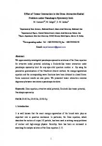
Our calculations are based on a finite range effective force widely used in HF calculations, the B1 interaction of Brink and Boeker [7] which was constructed to reproduce the experimental binding energies of 4 He, 16 O and 40 Ca. With this interaction we have performed HF calculations also for 12 C, 14 C, 48 Ca and 208 Pb nuclei. A comparison between the binding energies obtained in our calculations with the experimental values [11] is given in table 1. While the energies of 4 He, 16 O and 40 Ca are rather well reproduced, the model fails in describing those of the other nuclei. A study of the contribution of the four components of the force shows that only the spin–isospin (p=4) term provides attraction. The contribution of the isospin (p=2) and spin (p=3) channels is the same for the Z = N nuclei. Since in the present calculations protons and neutrons sp wave functions are identical, for Z = N nuclei the proton and neutron densities are equal, therefore the direct isospin term, eq. (9), is zero and the two exchange terms for p=2 and p=3, give the same result. Of course this picture breaks down for nuclei with neutron excess like 14 C, 48 Ca and 208 Pb. To investigate the influence of the tensor component of the force on HF calculations we have added to the B1 interaction the tensor force obtained from the Argonne v14 potential [8] and that obtained from the J¨ ulich–Stony Brook (JSB) interaction [6]. The tensor terms of the JSB interaction are constructed by considering the exchange of the π plus ρ mesons, therefore they are active only in the tensor isospin channel. On the other hand, the pure tensor term of the Argonne potential is very small if compared with the tensor-isospin one. For this reason in our calculations we have used only the tensor-isospin terms of the two interactions. These terms are shown in the panel (a) of fig. 1. This treatment of the tensor part of the interaction reproduces rather well the tensor terms of an effective interaction calculated within a Brueckner G-matrix approach. In ref. [12] is it shown that the effective force in the tensor channels is very similar to the bare nucleon–nucleon interaction. From fig. 1 the similarity between the JSB and Argonne tensor isospin channels is evident in the low momentum region. We did not use the full Argonne and JSB interactions because they are not suited for HF calculations. The Argonne potential is a realistic nucleon–nucleon interaction which reproduces the experimental data of the two nucleon systems, and therefore it has a strong repulsive core. With this interaction we have calculated 16 O and 40 Ca and both of them are unbound (52.08 and 217.18 MeV respectively). The JSB interaction is an effective force designed to describe low–lying excited states within the Landau–Migdal theory of finite Fermi systems, and for HF calculation it turns out to be too attractive. The binding energies obtained with the interactions constructed by adding to the B1 interaction the tensor terms of the Argonne v14 potential (A) and that of the JSB interaction (JSB) are shown in table 2. A comparison with the results of table 1 shows that the contribution of the tensor force is very small. The set of sp energies for the nuclei we have studied is shown in tables 3–7. For brevity we do not show these energies for the 208 Pb case. One can notice that in the 16 O and 6

40

Ca nuclei, the sp energies of the spin–orbit partner levels are the same, while for and 48 Ca they are different.

14

C

This results can be understood analyzing eq. (16). If the r–dependent terms would be constant, the angular momentum sums for nuclei having spin–orbit partner states occupied would be exactly zero. In reality each term is identified by small variations produced by the integral on q, depending from L and L′ and the integral on r depending from the sp wave functions. These variations are not large enough to prevent big cancelations between the contribution of the spin–orbit partners terms. The contribution of the tensor interaction can be significant in nuclei where not all the sp spin–orbit partners levels are occupied. In closed shell nuclei there are at most two of such a levels, one for neutrons and one for protons. The contribution of the tensor channel should be compared with that of the other channels where all the sp states contribute. In light nuclei, like 12 C, the tensor interaction could produce a noticeable contribution if compared with that generated by the other channels of the force which involves few sp levels. We expect that in heavier nuclei the tensor contribution produced by only one sp level should be compared with that produced by the other, many, sp levels for the central channels of the force. For this reason in the tables 3–7 the effect of the tensor force is noticeable only for those nuclei having spin–orbit partners not fully occupied. It is interesting to notice that the spin–orbit splitting produced by the tensor force goes in the opposite direction with respect to the experimental one. Clearly, a more realistic description of the nuclear ground state in terms of mean field model requires the presence of explicit spin–orbit terms in the interaction. In order to test the sensitivity of the 12 C ground state properties to the tensor interaction we have inserted a tensor–isospin channel of gaussian shape (in coordinate space) whose parameters have been fixed to reproduce the experimental binding energy of this nucleus. This new tensor force is shown in the panel (b) of fig. 1 and the results obtained with this new interaction for the other nuclei are shown in the tables by the columns labeled T6. It is worth to notice that this interaction has opposite sign with respect to the tensor terms of the JSB and Argonne interaction and a much stronger strength. The comparison done in table 2 between the binding energies obtained with this new interaction with those previously obtained shows that only the results of the two carbon isotopes have been strongly modified. In this table we see that the binding energies of the nuclei with all spin–orbit partners levels occupied are very little modified by the tensor force. The 48 Ca and 208 Pb nuclei show more sensitivity to the modification of the tensor component of the force, but it is however rather small. The same kind of effects can be seen in the other tables showing the sp energies. The sp energies of 12 C and 14 C nuclei are strongly modified by the new tensor force, but those of 16 O and 40 Ca remain the same. In 48 Ca the modification of the sp energies are relevant, even though the change on the binding energy is very small (∼ 2%). In order to see how the modification of the tensor interaction can affect the sp wave functions we have calculated the nucleon distributions. As example of the results obtained we show in fig. 2 the proton distributions of the 12 C, 14 C, 40 Ca and 48 Ca nuclei. On the 7

scale of the figure the curves representing the Argonne and JSB results are overlapped to the curves of the B1 results. The figure shows that the JSB and Argonne tensor potentials do not produce sizeable effects on the proton distributions. The situation is quite different when the T6 tensor terms is used. The proton distribution of 12 C and 14 C are quite different, while the effect on 40 Ca and 48 Ca are negligible. These results confirm the previous analysis on the behaviour of the tensor interaction. The tensor force plays an important role in 12 C and 14 C, but its effects are essentially zero for nuclei with fully occupied spin–orbit partner levels, and very small for medium–heavy nuclei.

4

Conclusions

In this work we have studied the effects of the tensor interaction on HF calculations. We found that there are big cancelations between the contributions of sp levels which are spin–orbit partners. For this reason, only the contribution of those sp states not having occupied the spin orbit partner level is significant. A closed shell nucleus can have at most two of these states, one for protons and one for neutrons, and, as a consequence, the effect is relatively small in heavy nuclei where it has to be compared with the effect of the other terms of the force active on all the sp levels. The situation is different for 12 C where only two levels are occupied, therefore, as we have shown, the effect of the tensor interaction is comparable with that of the other terms. One may argue whether the difficulties in reproducing the 12 C properties of traditional HF calculations can be overcome by inserting the tensor terms of the interaction. We have shown that, if these terms are included, it is possible to reproduce the 12 C binding energies without spoiling the agreement obtained for the other nuclei. To obtain this results the use of tensor forces very different from those of Argonne and JSB interactions has been necessary. On the other hand, the study of excited low-lying magnetic states [13] gives strong indications that the effective tensor isospin interaction should be quite similar to those of the Argonne and JSB interactions. The unified description of ground and excited nuclear states within a Hartree-Fock plus Random Phase Approximation theoretical scheme, rules out the possibility of fixing the tensor part of the effective interaction with a fit to the 12 C ground state properties. The task of constructing a new finite–range interaction to be used in mean field calculations was beyond the aim of the present paper, and it will be pursued in the future, by adding finite range spin–orbit and density dependent terms. In any case the results we have presented show the need of including tensor terms in this effective interaction if one wants the model to be valid on the full isotope table.

References [1] Kellog J., Rabi I., Ramsey N. and Zacharias J., Phys. Rev., 57 (1939) 677; Nordsieck A., Phys. Rev., 58 (1940) 310. 8

[2] Rarita W. and Schwinger J., Phys. Rev., 59 (1941) 436; Phys. Rev., 59 (1941) 556. [3] Bergervoet J.R., van Campen P.C., Klomp R.A.M., de Kok J.L., Rijiken T.A., Stocks V.G.J. and de Swart J.J., Phys. Rev. C, 41 (1990) 1435; Stocks V.G.J., Klomp R.A.M., Rentmeester M.C.M. and de Swart J.J., Phys. Rev. C, 48 (1993) 792; Wiringa R.B., Stocks V.G.J. and Schiavilla R., Phys. Rev. C, 51 (1995) 38. [4] Fabrocini A., Arias de Saavedra F., Co’ G. and Folgarait P., Phys. Rev. C, 57 (1998) 1668; [5] Wiringa R.B., Ficks V., Fabrocini A. Phys. Rev. C, 38 (1988) 1010. [6] Speth J., Klemt V., Wambach J. and Brown G.E., Nucl. Phys. A, 343, (1980) 382. [7] Brink D.M. and Boeker E., Nucl. Phys. A, 91 (1967) 1. [8] Wiringa R.B., Smith R.A. and Ainsworth T.L., Phys. Rev. C, 29 (1984) 1207. [9] Ring P. and Schuck P., The nuclear many body problem (Springer–Verlag, New York) 1980. [10] Guardiola R. and Ros J., Jour. Comp. Phys., 45 (1982) 374; Jour. Comp. Phys., 45 (1982) 390; Guardiola R., Schneider H. and Ros J., Anales de F´ısica A, 78 (1982) 154. [11] Audi G. and Wapstra A.H., Nucl. Phys. A, 565 (1993) 1. [12] Nakayama K., Krewald S., Speth J. and Love G., Nucl. Phys., A431 (1984) 419. [13] G. Co’ and Lallena A.M., Nucl. Phys. A, 510 (1990) 139; Lallena A.M., Phys. Rev. C, 48 (1993) 344.

9

Table 1: Binding energies, in MeV, obtained with the B1 interaction. The experimental values are taken from ref. [11]. 4

He C 14 C 16 O 40 Ca 48 Ca 208 Pb 12

exp B1 -28.30 -28.22 -92.16 -48.68 -105.28 -74.49 -127.62 -113.55 -342.05 -340.75 -416.00 -362.82 -1636.45 -2059.55

Table 2: Binding energies, in MeV, obtained with the interaction obtained by adding to the B1 interaction the tensor terms of ref. [6] (JSB) and that of ref. [8] (A). The column labeled T6 shows the results obtained with the tensor force adjusted to reproduce the experimental value of the 12 C binding energy. 4

He C 14 C 16 O 40 Ca 48 Ca 208 Pb 12

JSB A T6 -28.22 -28.22 -28.22 -47.17 -47.46 -92.36 -74.56 -74.59 -90.45 -114.10 -114.10 -113.53 -342.40 -342.40 -340.75 -364.01 -363.98 -377.01 -2074.51 -2074.00 -2063.93

Table 3: Single particle energies, in MeV, for 12 C for the interactions used. Since these calculations have been done without the Coulomb interaction, proton and neutron single particle energies are the same. 12

C

1s1/2 1p3/2

B1 JSB A T6 -36.81 -36.66 -36.55 -42.02 -11.82 -11.29 -11.36 -25.82

10

Table 4: Single particle energies, in MeV, for and with ν the neutron levels. 14

C

1s1/2 π 1p3/2 π 1s1/2 ν 1p3/2 ν 1p1/2 ν

B1 -44.83 -18.09 -40.55 -15.05 -15.05

14

JSB -44.93 -17.98 -40.62 -14.76 -15.77

C. We have indicated with π the proton A -44.93 -18.00 -40.61 -14.81 -15.66

Table 5: Same as table 3 for 16

O 1s1/2 1p3/2 1p1/2

Ca 1s1/2 1p3/2 1p1/2 1d5/2 1d3/2 2s1/2

16

O.

B1 JSB A T6 -49.40 -49.55 -49.55 -49.39 -21.71 -21.79 -21.79 -21.71 -21.71 -21.79 -21.79 -21.71

Table 6: Same as table 3 for 40

T6 -44.24 -25.65 -42.21 -25.26 -16.91

B1 -71.34 -45.24 -45.24 -21.19 -21.19 -20.17

JSB -71.57 -45.39 -45.39 -22.04 -22.04 -20.26

11

A -71.57 -45.39 -45.39 -22.04 -22.04 -20.26

40

Ca.

T6 -71.34 -45.24 -45.24 -21.95 -21.95 -20.17

Table 7: Same as table 4 for 48

Ca 1s1/2 π 1p3/2 π 1p1/2 π 1d5/2 π 1d3/2 π 2s1/2 π 1s1/2 ν 1p3/2 ν 1p1/2 ν 1d5/2 ν 1d3/2 ν 2s1/2 ν 2f7/2 ν

B1 -73.87 -50.81 -50.81 -28.95 -28.95 -26.96 -69.57 -45.44 -45.98 -23.64 -24.47 -22.94 -4.19

JSB -74.08 -50.56 -51.03 -28.72 -29.50 -27.54 -69.78 -45.49 -46.27 -23.57 -24.78 -23.03 -4.06

12

A -74.07 -50.53 -51.06 -28.70 -29.50 -27.48 -69.77 -45.47 -46.29 -23.55 -24.79 -23.29 -4.05

48

Ca. T6 -74.43 -51.76 -51.04 -34.07 -22.45 -26.96 -70.06 -44.96 -48.87 -25.87 -21.74 -22.88 -7.57

Figure Captions Figure 1: Tensor isospin terms added to the B1 interaction. In the panel (a) the curve labeled with A represents the term of the Argonne v14 potential [8], that labeled as JSB the term of the J¨ ulich–Stony Brook interaction of ref. [6]. The panel (b) shows the interaction adjusted to reproduce the 12 C experimental binding energy.

Figure 2: Proton density distributions obtained with the B1 interaction (full lines) with the A interaction (dashed lines), with the JSB interaction (dotted–dashed lines and with the T6 interaction (doubly dotted–dashed lines). On the scale of the figure the A and JSB results are overlapped.

13

100

A

3

[MeV fm ]

50

0

JSB

-50

(a) -100 0.0

1.0

2.0

3.0

4.0

5.0

-1

q [fm ] 2000 (b)

T6

3

[MeV fm ]

1500

1000

500

0 0.0

1.0

2.0

3.0 -1

q [fm ]

14

4.0

5.0

0.08

0.16

12

C

40

0.12

Ca

-3

ρ [fm ]

0.06

0.04

0.08

0.02

0.04

0.00

0.00 1.0

2.0

3.0

4.0

5.0

6.0

0.0

1.0

2.0

3.0

4.0

5.0

6.0

5.0

6.0

15

0.0 0.08

0.16

14

C

48

0.12

Ca

-3

ρ [fm ]

0.06

0.04

0.08

0.02

0.04

0.00

0.00 0.0

1.0

2.0

3.0 r [fm]

4.0

5.0

6.0

0.0

1.0

2.0

3.0 r [fm]

4.0