Test-Based Inference of Polynomial Loop-Bound Functions ∗ Olha Shkaravska
Rody Kersten
Marko van Eekelen
Radboud University Nijmegen {shkarav,r.kersten}@cs.ru.nl
Abstract This paper presents an interpolation-based method of inferring arbitrary degree loop-bound functions for Java programs. Given a loop, by its “loop-bound function” we mean a function with the numeric program variables as its parameters, that is used to bound the number of loop-iterations. Using our analysis, loopbound functions that are polynomials with natural, rational or real coefficients can be found. Analysis of loop bounds is important in several different areas, including worst-case execution time (WCET) and heap consumption analysis, optimising compilers and termination-analysis. While several other methods exist to infer numerical loop bounds, we know of no other research on the inference of non-linear loopbound functions. Additionally, the inferred bounds are provable using external tools, e.g. KeY. To infer a loop-bound function for a given loop it is instrumented with a counter and executed on a well-chosen set of values of the numerical program variables. By well-chosen we mean that using these test values and the corresponding values of the counter, one can construct a unique interpolating polynomial. The uniqueness and the existence of the interpolating polynomial is guaranteed if the input values are in the so-called NCA-configuration, known from multivariate-polynomial interpolation theory. The constructed interpolating polynomial presumably bounds the dependency of the number of loop iterations on arbitrary values of the program variables. This hypothesis is verified by a third-party proof assistant. A prototype tool has been developed which implements this method. This prototype can infer piecewise polynomial loop-bound functions for a large class of loops in Java programs. Applicability of the prototype has been tested on a series of safety-critical case studies. For most of the loops in the case studies, loop-bound functions could be inferred (and verified using a proof assistant). Categories and Subject Descriptors F.3.1 [LOGICS AND MEANINGS OF PROGRAMS]: Specifying and Verifying and Reasoning about Programs; D.2.4 [SOFTWARE ENGINEERING]: Software/Program Verification General Terms Verification, Performance, Reliability ∗ This
work was funded by the Artemis Joint Undertaking in the CHARTER project, grant-nr. 100039, and the Laboratory for Quality Software (LaQuSo).
Permission to make digital or hard copies of all or part of this work for personal or classroom use is granted without fee provided that copies are not made or distributed for profit or commercial advantage and that copies bear this notice and the full citation on the first page. To copy otherwise, to republish, to post on servers or to redistribute to lists, requires prior specific permission and/or a fee. PPPJ ’10, September 15–17, 2010, Vienna, Austria. c 2010 ACM 978-1-4503-0269-2. . . $10.00 Copyright
Radboud University Nijmegen and Open Universiteit
[email protected]
Keywords Loop-bound function inference, Program verification, Polynomial interpolation, NCA-configuration, Termination, JML
1.
Introduction
Loop-bounds are important in several different fields. The most obvious are worst-case execution time (WCET) and heap consumption analysis. Both are key issues for safety-critical systems, e.g. automotive and avionics applications. Compiler optimisations that transform loops, e.g. loop-unrolling, may also depend on knowledge about loop-bounds. Furthermore, termination of a program can only be proved if an upper bound on the number of loop iterations exists for each loop in the program. In the presented paper we describe test-based inference of piecewise polynomial loop-bound functions for Java loops with firstorder numerical loop conditions. Given a program with a loop, the corresponding loop-bound function (LBF) expresses an upper bound on the number of the loop iterations depending on (some of) the numerical program variables and data sizes. A similar term that is often used is “ranking function”. However, because our definition is more specialised (we consider only loops) and to avoid confusion with the term of the same name used in the information retrieval community, we prefer the term “loop-bound function”. Consider for example the loop in Listing 1. While several other methods exist that are able to infer a numerical loop bound for certain values of i, for instance minimal or maximal values, we infer the loop-bound function 15-i, which can be used to bound (or in this case, calculate exactly) the number of iterations of this loop for arbitrary values of i. Only one other paper [9] is known to the authors where symbolic bounds are inferred, but there only a limited use of non-linear terms in bounds is possible. In other articles, soundness is not usually discussed, but the correctness of the LBF inferred by the presented method can be checked by external tools. By proving correctness of the bound, termination of the loop is also proved inherently. 1 while ( i < 1 5 ) { 2 i ++; 3 }
Listing 1. A typical single (i.e. not nested) while-loop. The schema of our approach is as follows. Given a loop, it is first placed into a testing method. The loop in this method is instrumented with a counter and this testing method outputs the number of iterations of the loop on given values of the program variables. In this paper, we take into consideration numerical program variables that occur in the loop condition and its body. Then, the method is executed on a well-chosen set of inputs, which we call test values or, sometimes, following polynomial-interpolation terminology, test nodes. By well-chosen set of test values we mean that using these test values and the corresponding values of the counter, one can construct a unique interpolating polynomial. The uniqueness and
the existence of the interpolating polynomial is guaranteed if the input values are in the so-called NCA-configuration, known from multivariate-polynomial interpolation theory. This issue is highlighted in Section 2, explaining application of polynomial interpolation. The obtained data are used to compute the corresponding interpolating polynomial. The inferring part of the procedure outputs a method, annotated with the inferred bound, e.g. annotated in JML [15] by the decreases-expression. The correctness of the annotation is verified by an external checking tool. In our prototype implementation the method with the annotated loop is run through KeY [3], which contains a verification-condition generator and a theorem prover. To obtain concrete loop bounds (i.e. the concrete number of iterations on concrete data) , the obtained LBF may be applied to the results of data-flow analysis, possibly accelerated by abstract interpretation and/or program slicing. Several examples exist in the literature [7, 14] indicating how this might be implemented. This work builds on our previous research on size analysis [17], where we studied polynomial dependencies of the sizes of output data structures (e.g. the length of a linked list) on the sizes of input data structures. A similar algorithm as is used here for generating loop bounds was used in [18] to infer size relations. The running example throughout this paper is a while-loop with a quadratic LBF, given in Listing 2. This bound is successfully inferred by the prototype implementation and can be verified using KeY. 1 while ( x>0 && i>0 && i0 && j 2 the NCA is defined inductively on k. A set of Ndk nodes is in NCA in Rk if and only if • there is a (k − 1)-dimensional hyperplane such that it contains
some Ndk−1 of the given nodes lying in (k − 1)-dimensional NCA for the degree d, • there is a (k − 1)-dimensional hyperplane such that it contains k−1 some Nd−1 nodes, lying in (k − 1)-dimensional NCA for the degree d − 1, and these nodes do not lie on the previous hyperplane,
• in general, for any 0 ≤ i ≤ d, there is a (k − 1)-dimensional k−1 hyperplane such that it contains some Nd−i nodes, lying in (k − 1)-dimensional NCA for the degree d − i, and these nodes do not lie on the previous hyperplanes,
• thus, the remaining 1 node lies on the remaining hyperplane 1 http://charterproject.ning.com/
and does not belong to the previous ones.
For instance, for the example in Listing 2, we might assume that the loop-bound function is a quadratic polynomial (so, d = 2) and depends on three variables,`x,´ i and j. Recall, that a quadratic function of three variables has 53 = 10 coefficients: p(x, i, j) = a200 x2 + a020 i2 + a002 j 2 + a110 xi + a101 xj + a011 ij + a100 x + a010 i + a001 j + a000 . Therefore we need 10 three-dimensional points in R3 -NCA. According to the definition above we need: ` ´ • A set of 2+2 = 6 points on a plane in R2 -NCA: we take the 2 hyperplane j = 1 and the following nodes: x 2 3 4 3 4 4
i 1 1 1 2 2 3
i 1 1 2
3 2 1
j 1 1 1 1 1 1
0
These points are given (projected on the hyperplane j = 1) in Figure 1. ` ´ • A set of 2+1 = 3 points in R2 -NCA on another plane: we 2 take the hyperplane j = 2 and nodes x 3 4 3
i
j 2 2 2
1
2
= 1) point on yet another plane in R2 -NCA: 2 we take just (x = 4, i = 1, j = 3).
Java source Test-based inference procedure (the presented paper)
The corresponding system of linear equations is:
> > > > > > > > > > > > > > > > > > > > > > > > > > > > > > > > > > > > > :
=2 =6
Rejection: repeat testing with a higher degree
Annotated generated method with the chosen loop
= 12 =3
External checking tool Not verifiable automatically Verification Condition Prove manually
=8 =4 =5
Verified loop bound
= 11 =2 = 10
Its solution is (1, 0, 0, −1, 0, 0, 0, 0, 0, −1, 1), which yields the polynomial p(x, i, j) = x2 − xi − j + 1.
3.
x
the condition contains disjunctions is discussed in Section 5. Note that the limiting the loop-conditions to linear (in)equalities does not mean limiting to linear LBFs. The loop in Listing 2 has a non-linear LBF for instance.
`2+0´
22 a200 + 12 a020 + 12 a002 + 2a110 + 2a101 + 1a011 + 2a100 + 1a010 + 1a001 + 1a000 32 a200 + 12 a020 + 12 a002 + 3a110 + 3a101 + 1a011 + 3a100 + 1a010 + 1a001 + 1a000 42 a200 + 12 a020 + 12 a002 + 4a110 + 4a101 + 1a011 + 4a100 + 1a010 + 1a001 + 1a000 32 a200 + 22 a020 + 12 a002 + 3 · 2a110 + 3a101 + 2a011 + 3a100 + 2a010 + 1a001 + 1a000 42 a200 + 22 a020 + 12 a002 + 4 · 2a110 + 4a101 + 2a011 + 4a100 + 2a010 + 1a001 + 1a000 42 a200 + 32 a020 + 12 a002 + 4 · 3a110 + 4a101 + 3a011 + 4a100 + 3a010 + 1a001 + 1a000 32 a200 + 12 a020 + 22 a002 + 3a110 + 3 · 2a101 + 2a011 + 3a100 + 1a010 + 2a001 + 1a000 42 a200 + 12 a020 + 22 a002 + 4a110 + 4 · 2a101 + 2a011 + 4a100 + 1a010 + 2a001 + 1a000 32 a200 + 22 a020 + 22 a002 + 3 · 2a110 + 3 · 2a101 + 2 · 2a011 + 3a100 + 2a010 + 2a001 + 1a000 42 a200 + 12 a020 + 32 a002 + 4a110 + 4 · 3a101 + 3a011 + 4a100 + 1a010 + 3a001 + 1a000
4
Figure 1. An example of well-chosen test nodes for a polynomial g(x, i) = a20 x2 + a11 xi + a02 i2 + a10 x + a01 i + a00 . These may be used to reconstruct a polynomial g(x, i) = p(x, i, 1), where p is the polynomial bound for our running example. The grey area represents points that satisfy the condition x < i.
• A single (
8 > > > > > > > > > > > > > > > > > > > > > > > > > > > > > > > > > > > > >
0 && i > 0 && i < x && j > 0 && j 0 && i > 0 && i < x && j > 0 && j count =2 x=3, i=1, j=1 => count=6 x=4, i=1, j=1 => count=12 x=3, i=2, j=1 => count=3 x=4, i=2, j=1 => count=8 x=4, i=3, j=1 => count=4
nd
2 group: degree 1 NCA on plane x=3, i=1, j=2 => count=5 x=4, i=1, j=2 => count=11 x=3, i=2, j=2 => count=2 rd
3 group: degree 0 NCA on plane x=4 i=1, j=3 => count=10
We have reduced this task to the following one: construct an integer grid in Rk , such that it is based on d + 1 parallel hyperplanes and contains Ndk nodes, where • there are some Ndk−1 nodes in (k − 1)-dimensional NCA for
the degree d that lie on one of the hyperplanes and satisfy the corresponding projection of C to this hyperplane, k−1 • there are some Nd−1 nodes in (k − 1)-dimensional NCA for
Find the interpolating polynomial and generate the method annotated with the corresponding loop bound: p(x, i, j) = x*x – x*i – j + 1;
Figure 3. Test-based inference module in more detail. The choice of test nodes is explained in Section 2.
the degree d − 1 that lie on another hyperplane and satisfy the projection of C on this hyperplane,
k−1 • there are some Nd−i nodes in (k − 1)-dimensional NCA for
the degree d − i that lie on a fresh hyperplane and satisfy the projection of C on this hyperplane, 0 ≤ i ≤ d,
• and the remaining 1 node lies on the remaining hyperplane and
satisfying the corresponding projection of C. numerical variables that occur in the loop condition and in its body. In Section 8.2, we discuss a combination with program slicing techniques, which would yield exactly the variables on which the loop bound depends. The new method is now executed for a given degree and an appropriate set of values of these parameters, i.e. on so called test nodes. For instance, in our running example (x = 2, i = 1, j = 1) is an admissible test node. A well-chosen complete set of test nodes for this loop is given in the figure. The set consists of 10 nodes, since a polynomial of degree 2 of 3 variables has 10 coefficients: p(x, i, j) = a200 x2 + a020 i2 + a002 j 2 + a110 xi + a101 xj + a011 ij + a100 x + a010 i + a001 j + a000 . The result of a test run is the number of iterations for the corresponding node. For instance, with (x = 2, i = 1, j = 1) the loop body is executed 2 times, so the test method returns count = 2. From the results of the test-runs a polynomial over the parameters can be calculated which interpolates the test results. Multiple tactics are possible to guess the degree of the polynomial. It can be left to the user to supply it as input to the procedure, or an increasing degree can be tried, up to a certain bound. When a degree that is too low is supplied, the method will still find an LBF, but the checker will reject it. When a degree that is too high is given, the right polynomial will still be found, but more test-runs are needed. 3.1
LBF Inference: The Basic Method
This polynomial interpretation method was already applied to Size Analysis in previous work [17, 18]. The main challenge we face when we adjust the interpolation theory to inferring imperative loop-bound functions is that test data must not only lie on a grid (or more generally, be in NCA), but also satisfy the loop condition C. In Figure 1 we show the set of points satisfying the (in)equalities i < x, i > 0 and x > 0. This corresponds to the loop condition in our running example for the fixed j = 1. Whenever the loop condition is violated the loop is not executed and the testing method, which is wrapped around the loop, outputs 0. Therefore, if we con-
In general terms, our approach is based on search of the appropriate nodes on hyperplanes x1 = i0 , . . . , id . The search is inductive on the number of variables k. To bound the search space one uses an external optimisation procedure solving tasks of the form f (x1 , . . . , xk ) → min, where x1 , . . . , xk satisfy the constraints C(x1 , . . . , xk ). Currently in our prototype we use a linear programming solver, and therefore, the prototype handles only linear loop conditions. In general, one may use non-linear optimisation software, such as the implementation of the Augmented Lagrangian Genetic Algorithm (ALGA) by MathWorks 2 or the open-source Java package Sigoa 3 . The rest of this subsection is structured as is the inference procedure: generating test-nodes, conducting the tests and interpolating a polynomial LBF. 3.1.1
The algorithm for generating test-nodes
1. Run the chosen optimisation procedure for the objective functions xi → min, xi → max and the constraints constituted from the loop conditions and the additional bounds mi ≤ xi ≤ Mi , where mi , Mi are predefined resp. minimal and maximal admissible values of the variables xi , with 1 ≤ i ≤ k. The results define the k-dimensional box, that bounds the set defined by C (within the minimal-maximal values). We only look for nodes inside this box, because we know that others do not satisfy the loop condition. 2. Obtain search hyperplanes Hj by cutting the bounding box on d congruent “slices”, j = 0, . . . , d. 3. Amongst these hyperplanes, search for one that contains Ndk−1 nodes in (k − 1)-dimensional NCA for the degree d and the projection of C on this hyperplane, etc. as explained above. 2 http://www.mathworks.com/access/helpdesk/help/toolbox/
gads/bqf8bdd.html 3 http://sigoa.sourceforge.net/
Generated m Generated with the loop with the lo
/*@ assigna /*@ assig @ decrease @ decrea @ loop_inva @*/@ loop_in @*/
4. If the search succeeds, then stop. Otherwise, refine the grid by increasing the number of hyperplanes (e.g. by decreasing the distance between them) and repeat the search for the refined grid. This procedure finds test-nodes that both satisfy the loop condition and lie in NCA, if they exist on a grid within the minimal-maximal values mi , Mi . It finds suitable test-nodes for the case-study examples. To refine the search algorithm, one may add other, than rectangular grids, kinds of NCA, like e.g. pencil configurations. 3.1.2
Run tests
When suitable test nodes have been selected, we can now run the tests. Of course, because the investigated loops are actually executed, termination of the inference procedure depends on termination of those loops. The LBF inference procedure terminates if the considered loop terminates for all inputs. Assuming that infinite loops are undesirable in general, but especially for loops for which one seeks to bound the number of iterations, “finding” non-termination for certain inputs is a valuable result in itself. An implementation can never conclude nontermination, but it may quit execution after a particular amount of time has passed and hint the user that there is a large chance that the loop does not terminate on the considered inputs. 3.1.3
Find the interpolating polynomial
When all the tests have produced iteration counts (i.e. all have terminated), then we can now fit a polynomial, which interpolates these results. Because the test-nodes satisfy NCA, we know that a single interpolating polynomial exists. 3.2
Dealing with LBFs with rational or real coefficients
As stated earlier, LBFs can be polynomials with coefficients that are natural, rational or real numbers. However, when a polynomial has rational or real coefficients, its result is not necessarily a natural number, which, of course, any estimate of a number of loop iteration must be. Consider for instance the loop in Listing 3. 1 while ( start < end ) { 2 start += 4 ; 3 }
Listing 3. An example with a loop-bound function that is a polynomial over rational coefficients d end−start e. 4
The exact number of iterations of this loop is given by In other words, when end − start does not equate to a natural number, for instance to 43 , it must be ceiled. Generally, when the coefficients of the polynomial LBF p(¯ z ) are not natural numbers, the actual bound should be read as dp(¯ z )e. When the coefficients are naturals, we omit the ceiling notation. 3.3
Expressing the LBF in JML
In this section we discuss how we can express the found LBF in JML, in order to be verified by an external tool. The result of our method is Java code annotated with JML, in which the inferred LBF is expressed. Loop-bound functions are most easily expressed in JML by defining a decreases clause on the loop. This is an expression which must decrease by at least 1 on each iteration, and remains greater than or equal to 0, see the JML reference manual [13]. It therefore forms an upper-bound on the number of iterations. We want an external tool to verify the LBF for the case where the loop condition initially holds, otherwise the decreases-clause is not guaranteed to be ≥ 0 initially (and the loop will iterate exactly 0 times). Therefore, the loop condition is added as a precon-
dition to the constructed method. The example from Listing 2 is shown in annotated form in Listing 4. 1 2 3 4 5 6 7 8 9 10 11 12 13 14
/ ∗@ r e q u i r e s x>0 && i >0 && i 0 && j 0 && i>0 && i0 && j d + 1 hyperplanes for a refined grid. P Similarly to the estimates above, the estimate is N (d, k) = di=0 (D “ + 1 − i)(N (d − i, k − 1) + 1) ≤ ` D2 ´k ” ` D2 ´ . After failing with the first (N (d, k−1)+1)O 2 = O 2 hyperplane collection, D takes consecutively the values 2(d + 1), 28 2(d + 1), ... 28i+1 (d + 1), with 0 ≤ i ≤ imax and for imax the following holds. It is such that 28imax +1 (d + 1) ≤ M + 1, where M is the (length of the) side of the bounding box, generated by the optimisation procedure on the first step. So, we obtain that 1 +1 imax ≤ (log2 M − 1). The worst-case time, when we have to d+1 8 go through all the possible cuts, is then Pimax “` (28i+1 (d+1))2 ´k ”
= i=0 2 P max O(2k (d + 1)2k ) ii=0 O(216k )i = ` (216k )imax +1 −1 ´ O 2k (d + 1)2k 216k −1
Taking into account the estimate for imax we obtain that N (d, k) does not exceed O
4.
“ 2 ”k “ M + 1 ”2k (d + 1)2 16 2 2(d + 1)
! =O
„“
”k 1 (M + 1)2 17 2
«
Prototype and Case Studies
We have created a prototype implementation of the method in Java. This prototype can be used to load Java source files, select a loop to analyse, input an expected degree, infer a loop-bound function (LBF) and output Java code containing JML annotations in order
Hunt et al DIANA CDx Total
Nr. of loops 2 4 38 44
Analysable 2 4 23 29
Percentage 100% 100% 61% 66%
Table 1. Summary of the cases studied.
The results are shown in Table 1. As can be read from the table, we can handle roughly two-thirds of the loops found in the case studies. This means that we can infer an LBF for these loops using our prototype and prove it using KeY. All of the found LBFs were linear, i.e. of degree one. In the case studies, apparently, enough test-nodes are found after just a few cuts of the k-dimensional search space. This leads us to believe that the average complexity of the method lies somewhere around O(D2k ) for D = 29 (d + 1), rather than near the worstcase complexity. For the examples in the case studies this amounts to approximately one second spent in LBF inference. KeY was able to prove all the LBFs fully automatically, for which it requires approximately 5 to 10 seconds.
5.
Extensions
Two extensions were made to the core method in order to deal with a greater class of loops. The first extension enables analysis of loops with disjunctions in their conditions. The second extension enables analysis of loops with conditionals (if-statements) inside their bodies. 4 http://diana.skysoft.pt/ 5 http://adam.lille.inria.fr/soleil/rcd/
5.1
Piecewise LBFs for disjunctive loop conditions
Here, we consider loop conditions in disjunctive normal form (DNF) over arithmetical (in)equalities: mi n _ `^ i=1
(elij b erij )
´
j=1
with b ∈ {, =, 6=, ≤, ≥}. Note that any expression in propositional logic can easily be converted into DNF, using the laws of distribution and De Morgans theorems. We transform the DNF loop condition into a DNF in which the conjuncts represent pairwise non-overlapping numeric sets. We use the fact that: _ _ ´ `^ B1 ∨ . . . ∨ Bn = Bi \ Bj I⊆{1,...,n},I6=∅
i∈I
j∈I¯
where I¯ denotes the complement of I in {1, . . . , n}. Formally, the operation for e.g. a two-conjunct DNF Vm2 Vm1disjunction-splitting i=1 A2i , where each Aji is an inequation, is defined i=1 A1i ∨ by V 1 Vm2 Vm1 ,m2 split( m i=1 A1i ∨ i=1 A2i ) := =1 A1i1 ∧ (¬A2i2 )∨ Vim1 1=1,i ,m22 A1i1 ∧ A2i2 ∨ 2 =1 Vim1 1=1,i ,m2 (¬A 1i1 ) ∧ A2i2 i1 =1,i2 =1 Together, the disjunctive conjuncts of a loop condition determine a piecewise LBF. Consider the example given in Listing 5. 1 while ( start 100), (start < end) ∧ (end > 100) ∧ ¬(end < 40) and (start < end) ∧ (end < 40) ∧ (end > 100). Since (end < 40) and (end > 100) cannot both be true, this can easily be simplified to the following two pieces: (start < end) ∧ (end < 40) and (start < end) ∧ (end > 100) Then it constructs test methods for two separate loops, one with each condition. From this point on, the regular inference procedure runs. It generates the following piecewise bound: 8 < end − start if (start < end) ∧ (end < 40) end − start if (start < end) ∧ (end > 100) : 0 else In this case the polynomials in both clauses of the disjunction coincide. Disjunction-splitting takes care of loop conditions containing disjunctions, as long as the body of the loop satisfies the following separated pieces property: For each disjunctive piece of the loop-condition, not overlapping any other pieces, the loop-body does not change the program variables in such a way that another piece becomes satisfied. An example of a loop that does not satisfy this property is given in Listing 6. 1 while ( i < 30 | | ( i > 29 && i < 1 0 0 ) ) 2 i ++;
Listing 6. Loop in which the pieces are separate, but a jump is made from one piece to the other
5.2
Branching inside the loop body
The basic procedure finds correct LBFs for most loops containing branching, such as for example the one in Listing 2. However, there are cases in which the basic procedure fails, because the different branches affect the bound in different ways. Such a case is shown in Listing 7. 1 while ( i > 0 ) 2 if ( i > 1 0 0 ) i −= 1 0 ; 3 else i −= 1 ;
Listing 7. Example where the basic method supplies an incorrect LBF. Therefore, branch-splitting is applied, yielding the untight, but correct LBF i. To solve this problem, we have invented branch-splitting. This procedure finds LBF for loops where the if-statements, if they exist in a loop body, have the following worst-case computation branch (WCCB) property: For each loop body, there is an execution path such that, for any collections of values of the loop variables, if one follows this execution path in every loop iteration one reaches the worst-case, i.e. the upper bound. With branch-splitting, we mean that we generate multiple new loops from the original, one for each possible branch. We then do the analysis for each of these branches. The LBF is then the maximum of all the inferred LBFs. Thanks to the WCCB property, we can easily find the LBF that always specifies the maximum, by supplying a set of values for the variables (say, all ones) to all the LBFs. For the example in Listing 7, this yields the LBF i. A simple sub-class of loops with the WCCB property is given by if-statements breaking the loop execution, by a return or break or by throwing an exception. An example is shown in Listing 8. 1 for ( int i = 0 ; i < a . length ; i ++) 2 if ( a [ i ] < b [ i ] ) return −1; 3 else if ( a [ i ] > b [ i ] ) return + 1 ;
Listing 8. In this loop removing the if-statement yields a loop with the exact loop-bound function a.length - i that is the same as the worst-case bound of the original loop. In general, in cases like this one may discard return-branches completely, since they do not yield an upper bound. Another simple sub-class of loops with the WCCB property is given by loops containing if-statements, such that for all branches the values of the loop counter are the same. This happens when in the if-statement the values of variables, on which a given loop condition depends, are not changed. This is the case, for instance, when in the if-statement one changes the values in an array but not its length. Note, that when the loop parameters are changed in the same way in both the if and the else clauses then the ifstatement may be transformed into an equivalent code fragment where it satisfies the condition above. An example that does not satisfy the WCCB property is shown in Listing 9. 1 while ( i > 0 ) 2 if ( i % 2 == 0 ) i −= 3 ; 3 else i ++;
Listing 9. Example that does not satisfy the WCCB property and is therefore not analysable using our method
C = C1 ᴠ ... ᴠ Ci ᴠ... ᴠ Cm where, Ci are disjoint: disjunction-splitting
C1
Cm
Ci
...
...
Basic procedure: the condition is a conjunction of a 1st-order arith. predicate
LB
C1 → q1
Ci → qi
...
branch-splitting
F
d cte reje Basic procedure: the loop body with the 1-st branch
...
Basic procedure: the loop body with the n-th branch
Ci → pi1
...
Ci → pin
Cm → qm
...
qi:=select-max(pi1, ...,pin)
(C1 → q1 ) ᴠ ... ᴠ (Ci → qi) ᴠ ... ᴠ (Cm → qm)
Figure 4. Overview of the inference procedure with extensions. This example does not satisfy the property because executing the else-branch exclusively would yield an infinite bound. Not that it would also be impossible to formulate a correct decreases-clause for this loop. An overview of the method with extensions is given in Figure 4. First we apply disjunction splitting, then we execute the basic method for each of the separate pieces. If this does not yet yield a correct LBF, then we apply branch-splitting and take the maximum of each of the LBFs of all the branches as LBF.
6.
Evaluation
There are still some examples in the case studies that cannot yet be analysed using our method. At this point, we do not consider cases where the loop bound depends on: • Fields of referenced objects • Method invocations • Booleans • Different threads
A way of handling bounds that depend on references is described in [1], which we might incorporate in the future. Furthermore, we require that the loops satisfy the separated pieces and worst-case computation branch properties. We believe that satisfying these properties is only a minor restriction, since rewriting loops to do so is usually fairly straight-forward. Such properties might even be including in the coding style requirements for safety-critical software.
For examples that can be handled by our method, it usually computes the exact LBF. An exception to this is when branch-splitting is applied. This means that compared to other methods, our method finds bounds that are equally tight, or tighter. Furthermore, other methods are unable to derive non-linear LBFs. This is discussed in more detail in the next section.
7.
Related Work
Various other research results on bounding the number of loop iterations exist. However, most are concerned with concrete (numerical) bounds, instead of loop-bound functions. Also, most can only handle (tightly) cases where the bound depends linearly on program variables (we can handle the polynomial case). In a sense, our technique is more general than the methods discussed in this section. It may not be the most efficient method for simple loops, but it can be used to handle certain more complex cases. This makes it complementary to the other techniques discussed here. Another common difference is that other approaches rely on handmade soundness proofs of their method, while we rely on a verification tool to ensure that the derived LBFs are correct. In [8], pattern-matching on abstract syntax trees (ASTs) is used by Fulara et al to select one of several syntax-based schemes for generating decreases-clauses. If the AST matches a given pattern, then parameters from this pattern can be used to form a decreases-clause. The authors claim to cover 71% of all for-loops in a set of case studies. It is thinkable that their method is used in an implementation for the basic cases and our method is applied when no pattern matches. Abstract interpretation, program slicing and invariant analysis are used by Ermedahl et al in [7] to infer numerical bounds for
C programs. The bounds meant here are integers representing the number of times a certain block of code is executed. The method can infer bounds for over 50% of the loops in a set of benchmarks. A similar approach is taken by Lokuciejewski et al in [14], who combine abstract interpretation with polytope models to calculate numerical loop bounds for C programs. Both upper and lower bounds are calculated and the analysis is accelerated by using program slicing. Even though there are restrictive constraints on the loops that can be analysed, the authors claim that they can handle 99% of all for-loops in a set of benchmarks. Soundness or verification of the bounds are not discussed. Abstract interpretation is also used in [6], in combination with flow analysis. Numerical bounds can be found for 84% of the loops in a benchmark suite. The method works on C programs. Gulwani uses “off-the-shelf linear invariant generation tools” to compute symbolic loop bounds in [9]. The authors experiment with different counter instrumentation methods and a technique they named “control-flow refinement”. Loop-bound functions are presented as right-hand sides of the inequations in loop invariants. Inference of invariants is based on linear arithmetic, but some limited use of non-linear terms is possible as well. Given a particular program, the base arithmetic may be extended by a finite set of non-linear operators together with reasoning rules for them. The inference system, first, introduces a fresh variable for each non-linear operator, then deals with linear combinations of such variables (and usual arithmetic variables). The operators and the rules are chosen e.g. by a user, who knows which sort of invariants one can expect in the given code. In a related article by the same author(s) [10], pattern-matching against known loop-iteration lemmas is used to establish bounds for C and C++ programs. This last method can find bounds for 93% of the loops in a significant Microsoft product. In [4], Ben-Amram describes a method to derive global ranking functions, based on Size-Change Termination. Such a ranking function is required to decrease in each basic block of the program. He uses an abstraction called Monotonicity Constraints and represents them as graphs. Various algorithms are described that can be applied to these graphs to judge termination and construct ranking functions. Hunt et al discuss the expression of manually conceived loopbound functions in JML, their verification using KeY and the combination with data-flow analysis in [11]. This article is an important motivation for our work. What is “missing” in the method is the automated inference of loop-bound functions, which we supply. In [2], Albert et al describe a system of generating and solving cost recurrence relations. These relations define functions that represent upper bounds on time or memory usage by a program. To solve a recurrence relation means to find a closed, i.e. a recursionfree, form of the corresponding function. Terms in the system represent monotonic real functions and, besides monotonically increasing polynomials, contain the exponent and the logarithmic functions.
8.
• as earlier, are in NCA configuration, • as earlier, satisfy the loop condition, • are of the form (
m m i1 , . . . , ik ). n n
Instead of an original loop condition P (x1 , . . . , xk ) consider the predicate P 0 (x01 , . . . , x0k ) = P (mx1 , . . . , mxk ). Using already existing part of the method, generate the intermediate list of integer nodes lying in NCA and satisfying this predicate: [(x011 , . . . , x01k ), . . . , (x0N 1 , . . . , x0N k )] The desirable list of test nodes is: [(mx011 , . . . , mx01k ), . . . , (mx0N 1 , . . . , mx0N k )] Indeed, the nodes in this list satisfy all three conditions above: • they obviously lie in NCA, since it is just scaling of another
NCA grid • each of them satisfies the loop condition, because this holds:
P (mx0j1 , . . . , mx0jk ) = P 0 (x0j1 , . . . , x0jk )
Future Work
Here we discuss some areas where we will improve and extend our research and the prototype implementation in the future. 8.1
by memorising hyperplanes that have enough points for exactly a degree d − i (see Section 3.1 for more detail). When inferring the LBF for a loop with an increment > 1 the method does not always generate correct bound functions. In the case of linear polynomials inferred bound functions are correct but not optimal. In general, for a given loop, the connection between its nonlinear upper bound function, its incremental step and the interpolating polynomial needs to be studied. We have done the study for linear bounds, but the results have not been implemented yet. Now we briefly discuss our observations about the connection between incremental steps and linear loop-bound functions. Strictly speaking, if m > 1 is an incremental step in a loop, then its worst-case bound is not exactly a polynomial but is of the form z) d p(¯ e. Depending on the test nodes, our method finds a bound of m the form p1 (¯ z ) + r, where 0 ≤ r ≤ 1. This can be explained by z) the fact that a graphical representation of d p(¯ e takes a step form, m where the steps are of size m. For the interpolation to be correct, all test-nodes must be m apart, such that they are located at the same point w.r.t. the begin of a step interval. Furthermore, it is possible to infer the optimal polynomial bound (i.e. not ceiled) when the right test-nodes are chosen. This bound is p(¯z)+(m−1) for LBF-s of the m aforementioned form. An example of such a loop is given in Listing 3. We want to choose such testing nodes (starti , endi ) that endi − starti mod 4 == 0. In other words, test-nodes must be multiples of the step. Then the upper bound is g(¯ z ) + 1 (or even g(¯ z ) + m−1 ), where g(¯ z ) is the data interpolating polynomial. We m have been working on the procedure of generating test nodes for loops with steps even of more general form m/n, where m > 1. The task task is formulated as follows: given a loop, one needs to generate the k-dimensional nodes, that:
Improving test-node search
The first step in improving the implemented generation of testnodes is to replace the linear programming solver that is used in the current prototype with a global optimisation library. This would enable us to handle loop conditions containing non-linear (in)equalities. Next, the implemented search algorithm may be optimised, first of all, in its searching hyperplane-by-hyperplane part, probably
• they are of the form (
m m i1 , . . . , ik ) because n n
(mx0j1 , . . . , mx0jk ) = (
m 0 m nxj1 , . . . , nx0jk ), n n
so il = nx0jl . In the example of this section we interpolate a linear polynomial of two variables p(start, end) = a · start + b · end + c, which has three coefficients. The intermediate test nodes satisfy the predicate 4 · start < 4 · end. They are, e.g. (0, 1), (0, 2), (1, 2). The corresponding test nodes are (0, 4) with the loop-iteration counter value 1, (0, 8), with the counter 2 and (4, 8) with the
counter 1. The corresponding interpolating polynomial is and a polynomial bound function is end−start + 34 . 4 8.2
end−start 4
Program slicing
As is done in [7] and [14], we intend to use program slicing to accelerate the analysis. This way, irrelevant parts of the code can safely be ignored. Slicing gives us exactly the variables on which the loop condition (i.e. the bound) depends. Since the complexity of our analysis is exponential in the number of variables in the polynomial, this is highly beneficial to the performance of the method. 8.3
Combination with data-flow analysis
The method could be combined with data-flow analysis in order to yield concrete numerical bounds. For example, when by flow analysis we can obtain an interval for each variable, then we can obtain a minimum and maximum on the number of loop iterations by searching for minima and maxima of the LBF within this interval. 8.4
Size and heap consumption analysis
The analysis should be combined with our previous research on size analysis. There is a mutual dependency between the two. What size analysis may add to LBF inference is that a loop bound often depends on the size of a data structure (e.g. the length of a list). If we can bound this size, then we can bound the number of loop-iterations. What LBF inference may add to size analysis is that often a data structure gets constructed by executing a loop. Think of iteratively adding elements to a list, for example when converting an array into a list object. If in that case we know the number of loop-iterations, we know the size of the constructed list. Furthermore, objects may be constructed in a loop. This means that LBF inference is also crucial to bound heap-space usage, which is a future goal for the CHARTER project.
9.
Conclusions
We have presented a way of computing arbitrary degree loopbound functions. By expressing these functions in JML their correctness can be proved, which is very valuable in safety-critical systems. While various other methods for inferring loop-bounds exist, we are not familiar with any other works on generating nonlinear loop-bound functions for Java. Moreover, the technique presented herein is largely complementary to other methods, since it is more general and can solve certain more complex cases, such as quadratic bounds. Using a prototype implementation, loop-bound functions can be inferred for 66% of all loops in a set of case studies from actual safety-critical systems.
References [1] E. Albert, P. Arenas, S. Genaim, and G. Puebla. Dealing with numeric fields in termination analysis of java-like languages. In FTfJP, pages 77–87, 2008. [2] E. Albert, P. Arenas, S. Genaim, and G. Puebla. Automatic inference of upper bounds for recurrence relations in cost analysis. In SAS, pages 221–237, 2008. [3] B. Beckert, R. H¨ahnle, and P. H. Schmitt, editors. Verification of Object-Oriented Software: The KeY Approach. LNCS 4334. SpringerVerlag, 2007. [4] A. M. Ben-Amram. Size-change termination, monotonicity constraints and ranking functions. In CAV, pages 109–123, 2009. [5] C. K. Chui and M.-J. Lai. Vandermonde determinants and lagrange interpolation in Rs . Nonlinear and convex analysis, pages 23–35, 1987.
[6] M. De Michiel, A. Bonenfant, H. Cass´e, and P. Sainrat. Static loop bound analysis of C programs based on flow analysis and abstract interpretation. In RTCSA ’08: Proceedings of the 2008 14th IEEE International Conference on Embedded and Real-Time Computing Systems and Applications, pages 161–166, Washington, DC, USA, 2008. IEEE Computer Society. ISBN 978-0-7695-3349-0. [7] A. Ermedahl, C. Sandberg, J. Gustafsson, S. Bygde, and B. Lisper. Loop bound analysis based on a combination of program slicing, abstract interpretation, and invariant analysis. In C. Rochange, editor, 7th Intl. Workshop on Worst-Case Execution Time (WCET) Analysis, Dagstuhl, Germany, 2007. Internationales Begegnungs- und Forschungszentrum f¨ur Informatik (IBFI), Schloss Dagstuhl, Germany. [8] J. Fulara and K. Jakubczyk. Practically applicable formal methods. In SOFSEM ’10: Proceedings of the 36th Conference on Current Trends in Theory and Practice of Computer Science, pages 407–418, Berlin, Heidelberg, 2010. Springer-Verlag. ISBN 978-3-642-11265-2. [9] S. Gulwani. SPEED: Symbolic complexity bound analysis. In CAV ’09: Proceedings of the 21st International Conference on Computer Aided Verification, pages 51–62, Berlin, Heidelberg, 2009. SpringerVerlag. ISBN 978-3-642-02657-7. [10] S. Gulwani, S. Jain, and E. Koskinen. Control-flow refinement and progress invariants for bound analysis. In PLDI ’09: Proceedings of the 2009 ACM SIGPLAN conference on Programming language design and implementation, pages 375–385, New York, NY, USA, 2009. ACM. ISBN 978-1-60558-392-1. [11] J. J. Hunt, F. B. Siebert, P. H. Schmitt, and I. Tonin. Provably correct loops bounds for realtime java programs. In JTRES ’06: Proceedings of the 4th international workshop on Java technologies for real-time and embedded systems, pages 162–169, New York, NY, USA, 2006. ACM. ISBN 1-59593-544-4. [12] T. Kalibera, J. Hagelberg, F. Pizlo, A. Plsek, B. Titzer, and J. Vitek. CDx : a family of real-time java benchmarks. In Proceedings of the 7th International Workshop on Java Technologies for Real-Time and Embedded Systems, JTRES 2009, Madrid, Spain, September 23-25, 2009, pages 41–50. ACM, 2009. [13] G. T. Leavens, E. Poll, C. Clifton, Y. Cheon, C. Ruby, D. Cok, P. M¨uller, J. Kiniry, and P. Chalin. JML Reference Manual. Draft Revision 1.200, Feb. 2007. [14] P. Lokuciejewski, D. Cordes, H. Falk, and P. Marwedel. A fast and precise static loop analysis based on abstract interpretation, program slicing and polytope models. In CGO ’09: Proceedings of the 7th annual IEEE/ACM International Symposium on Code Generation and Optimization, pages 136–146, Washington, DC, USA, 2009. IEEE Computer Society. ISBN 978-0-7695-3576-0. [15] E. Poll, P. Chalin, D. Cok, J. Kiniry, and G. T. Leavens. Beyond assertions: Advanced specification and verification with JML and ESC/Java2. In In Formal Methods for Components and Objects (FMCO) 2005, Revised Lectures, volume 4111 of LNCS, pages 342– 363. Springer, 2006. [16] T. Schoofs, E. Jenn, S. Leriche, K. Nilsen, L. Gauthier, and M. Richard-Foy. Use of PERC Pico in the AIDA avionics platform. In Proceedings of the 7th International Workshop on Java Technologies for Real-Time and Embedded Systems, pages 169–178. ACM, 2009. [17] O. Shkaravska, M. van Eekelen, and R. van Kesteren. Polynomial size analysis of first-order shapely functions. Logic in Computer Science, 2:10(5), 2009. [18] R. van Kesteren, O. Shkaravska, and M. van Eekelen. Inferring static non-monotonically sized types through testing. In 16th International Workshop on Functional and (Constraint) Logic Programming (WFLP’07), Paris, France, volume 216C of Electronic Notes in Theoretical Computer Science, pages 45–63, 2008.