Io e Physical-Technical Institute, 194021 St.-Petersburg, Russia. Kenneth M. ... averaged variation rate of the proton-to-electron mass ratio. We find j _=j < 1:510.
TESTING COSMOLOGICAL VARIABILITY OF THE PROTON-TO-ELECTRON MASS RATIO USING THE SPECTRUM OF PKS 0528{250 Alexander Y. Potekhin, Alexander V. Ivanchik, and Dmitry A. Varshalovich Io�e Physical-Technical Institute, 194021 St.-Petersburg, Russia
Kenneth M. Lanzetta
Astronomy Program, Department of Earth and Space Sciences State University of New York at Stony Brook, Stony Brook, NY 11794{2100, U.S.A.
Jack A. Baldwin
Cerro Tololo Inter-American Observatory, Casilla 603, La Serena, Chile
Gerard M. Williger
Goddard Space Flight Center, Code 681, NASA/GSFC, Greenbelt MD 20771, U.S.A. and
R. F. Carswell
Institute of Astronomy, Madingley Road, Cambridge CB3 0HA, U.K.
ABSTRACT
Multidimensional cosmologies allow for variations of fundamental physical constants over the course of cosmological evolution, and di�erent versions of the theories predict di�erent time dependences. In particular, such variations could manifest themselves as changes of the proton-to-electron mass ratio � = mp=me over the period of � 1010 yr since the moment of formation of high-redshift QSO spectra. Here we analyze a new, high-resolution spectrum of the z = 2:81080 molecular hydrogen absorption system toward the QSO PKS 0528{250 to derive a new observational constraint to the timeaveraged variation rate of the proton-to-electron mass ratio. We nd j�=� _ j < 1:5 � 10?14 yr?1, which is much tighter than previously measured limits. cosmology: observations { quasars: absorption lines { quasars: individual (PKS 0528{250) { atomic data
Subject headings:
1
1. INTRODUCTION
another technique, based on an analysis of H2 absorption lines only. One object suitable for such analysis is the z = 2:811 absorption system toward PKS 0528{250, in which Levshakov & Varshalovich (1985) identi ed molecular hydrogen absorption lines based on a spectrum obtained by Morton et al. (1980). Foltz, Chaffee, & Black (1988) have presented a limit to possible variation of � based on their observations of PKS 0528{250. Their analysis did not, however, take into account wavelength-to-mass sensitivity coe�cients, hence their result appeared to be not well grounded. Subsequently the spectrum of Foltz, Chaffee, & Black (1988) was reappraised by Varshalovich & Levshakov (1993), who obtained j��=�j < 0:005 at the redshift z = 2:811, and by Varshalovich & Potekhin (1995), who obtained j��=�j < 0:002 at the 2� signi cance level. (Here ��=� is the fractional variation of �.) More recently, Cowie & Songaila (1995) used a new spectrum of PKS 0528?250 obtained with the Keck telescope to arrive at the 95% con dence interval ?5:5 � 10?4 < ��=� < 7 � 10?4. Here we present a pro le tting analysis of a new, high-resolution spectrum of PKS 0528?250, obtained in November 1991 with the Cerro-Tololo InterAmerican Observatory (CTIO) 4 m telescope. We have calculated the wavelength-to-mass sensitivity coe�cients for a larger number of spectral lines and employed them in the analysis, which yields the strongest observational constraint yet to possible � variation over the cosmological time scale (eq. [9] below).
The possibility of the variability of fundamental physical constants was rst put forward by Dirac (1937) in the course of his discussion with Milne (1937). Later it was considered by Teller (1948), Gamow (1967), Dyson (1972) and other physicists. Interest in the problem increased greatly during the last decade, due to new developments in the Kaluza{ Klein and supergravity models of uni cation of all the physical interactions. Chodos & Detweiler (1980), Freund (1982), Marciano (1984), and Maeda (1988) discussed possibilities of including these multidimensional theories into the cosmological scenario of the expanding Universe and found that the low-energy limits to the fundamental constants might vary over the cosmological time. Variations of the coupling constants of strong and electroweak interactions might then cause the masses of elementary particles to change. Note that an increase of the proton mass by 0.08% would lead to transformation of protons into neutrons (by electron capture), resulting in destruction of atoms in the Universe. As demonstrated by Kolb, Perry, & Walker (1987) and Barrow (1987), observational bounds on the time evolution of extra spatial dimensions in the Kaluza{Klein and superstring theories can be obtained from limits on possible variations of the coupling constants. Damour & Polyakov (1994) have developed a modern version of the string theory which assumes cosmological variations of the coupling constants and hadron-to-electron mass ratios. Therefore the parameters of the theory can be restricted by testing cosmological changes of these ratios. The present value of the proton-to-electron mass ratio is � = 1836:1526645 (57) (CODATA, 1997). Obviously, any signi cant variation of this parameter over a small time interval is excluded, but such variation over the cosmological time � 1:5 � 1010 yr remains a possibility. This possibility can be checked by analyzing spectra of high-redshift QSOs. The rst analysis of this kind has been performed by Pagel (1977), who obtained a restriction j�=� _ j< 5 � 10?11 yr?1 on the variation rate of � by comparison of wavelengths of H I and heavy-ion absorption lines, as proposed by Thompson (1975). This technique, however, could not provide a fully conclusive result, since the heavy elements and hydrogen usually belong to di�erent interstellar clouds, moving with di�erent radial velocities. In this paper we use
2. OBSERVATIONS Observations were obtained with the CTIO 4 m telescope in a series of exposures of typically 2700 s duration totaling 33750 s duration. The CTIO Echelle Spectrograph with the Air Schmidt camera and Reticon CCD was used at the Cassegrain focus to obtain complete spectral coverage over the wavelength range � � 3465 ? 4905 � A. Observations of standard stars and of a Th-Ar comparison arc lamp were obtained at intervals throughout each night, and observations of a quartz lamp were obtained at the beginning or end of each night. For all observations, the slit was aligned to the parallactic angle. Data reduction was performed following procedures similar to those described previously by Lanzetta et al. (1991). One-dimensional spectra were extracted from the two-dimensional images using an optimal 2
comparison of the H2 laboratory wavelengths with the corresponding wavelengths for D2 and T2 molecules, which simulate just the mass variation of the study, and also for HD molecules. Varshalovich & Potekhin (1995) also removed some inaccuracies from the table of Varshalovich & Levshakov (1993). The two ways of performing the calculation yielded very similar Ki values, which argues that both are correct. For each electron-vibration-rotational band, a wavelength of a transition between two states with the vibrational and rotational quantum numbers v; J and v 0 ; J 0 can be presented as
extraction technique, and individual one-dimensional spectra were coadded using an optimal coaddition technique. Wavelength calibrations were determined from two-dimensional polynomial ts to spectral lines obtained in the Th-Ar comparison arc lamp observations. Continua were tted to the one-dimensional spectra using an iterative spline tting technique. The spectral resolution was measured from spectral lines obtained in the Th-Ar comparison arc lamp exposures. This is appropriate because for all observations the seeing pro le was larger than the slit width. The spectral resolution was found to be FWHM � 21 ? 24 km s?1 in the spectral intervals used for the analysis. Figure 1 presents parts of the spectrum, with the t superposed on the data, for several spectral intervals in which the H2 absorption lines have been analyzed (for more detail, see C� ircovi�c et al., 1998).
� � = �vu J 0
? �vl
00
J
00
�?1
(3)
;
where � is the level energy in cm?1 , and the superscripts u and l stand for the upper and the lower level, respectively. For each of them
3. SENSITIVITY COEFFICIENTS
�vJ =
The possibility of distinguishing between the cosmological redshift of the spectrum and wavelength shifts due to a variation of � arises from the fact that the electronic, vibrational, and rotational energies of a molecule each undergo a di�erent dependence on the reduced mass of the molecule. Hence comparison of the wavelengths of various electronic-vibrationalrotational molecular absorption lines observed in the spectrum of a high-redshift quasar with corresponding molecular lines observed in the laboratory may reveal or limit the variation of � with time. If the value of � at the early epoch z of the absorption spectrum formation were di�erent from the contemporary one, then the ratio � � (�i =�k )z ' 1 + (K ? K ) �� (1) i k (�i =�k )0 � would deviate from unity. Here Ki = d ln �i =d ln �
0
X
m;n
�
Ymn v +
� 1 m (J (J + 1))n : 2
(4)
We consider the Lyman bands (transitions X 1 �+g ! B 1 �+u ) and the Werner bands (X 1 �+g ! C 1 �+u ) of the molecular H2 spectrum. The parameters Ymn for the three corresponding states are taken from Huber & Herzberg (1979). The coe�cient Y00 is rede ned so that the energy of each rotational-vibrational band is counted from the ground-state energy. For the state �u , the factor J (J + 1) in the terms with n = 1 of equation (4) has been replaced by (J (J + 1) ? 1), in order to take into account the projection (�2 = 1) of the electron orbital moment on the molecular axis. From the Born{Oppenheimer approximation we conclude that the coe�cients Ymn are proportional to �?n?m=2 . Then the sensitivity coe�cients Ki are easily obtained from equations (2){(4): Kv J ?v J = �v J ?v J 0
0
00
00
where
(2)
kvJ =
is the coe�cient which determines the sensitivity of the wavelength �i of ith spectral line with respect to the variation of the mass ratio �. These coe�cients were calculated previously by Varshalovich & Levshakov (1993) from the spectroscopic constants of the H2 molecule, using the Born{ Oppenheimer approximation. Later Varshalovich & Potekhin (1995) calculated Ki in another way, by
X
m;n
0
0
�
00
?
kvu J
? kvl
�
;
(5)
� 1 m (J (J + 1))n ;
(6)
00
ymn v + 2
0
0
00
J
00
and the coe�cients ymn are given in Table 1 (in cm?1 ). For the state �u , the factor J (J + 1) in the terms with n = 1 has been replaced by (J (J +1) ? 1), as well as in equation (4).
3
Fig. 1.| Selected parts of the spectrum PKS 0528?250 with absorption lines of H2 molecules at the redshift z = 2:81080. The t is superposed on the data. The most distinct absorption lines of the Lyman band are labeled on the plot. The thick bars along the horizontal axes mark the spectral intervals used in the t (Sect. 4.1), and the asterisks mark the positions of individual lines listed in Table 2 and used in the independent analysis in Section 4.2 (note that there are other spectral intervals and lines included in the analyses but belonging to Lyman and Werner branches not shown in the gure). 4
4. RESULTS OF ANALYSIS 4.1. Synthetic spectrum analysis
We have applied to the spectrum a routine described previously by Lanzetta & Bowen (1992). This routine performs a comparison of the synthetic and observed spectrum and nds an optimal solution to a parameterized model of a set of absorption pro les, simultaneously taking account of all observed spectral regions and transitions. Parameter estimates are determined by minimizing �2 , and parameter uncertainties and correlations are determined by calculating the parameter covariance matrix at the resulting minimum. A total of 59 H2 transitions are incorporated into the �2 t, and the absorption lines corresponding to these transitions occur across the linear, saturated, and damped parts of the curve of growth. The redshift, Doppler parameter, and column densities of the H2 rotational levels J 00 = 0 through J 00 = 7 were adopted as free parameters. Wavelengths, oscillator strengths, and damping coe�cients of the H2 transitions were taken from Morton & Dinerstein (1976). According to C� ircovi�c et al. (1998), the total H2 column density is log N (H2 ) = 18:45 � 0:02 and the Doppler parameter is b = 3:23 � 0:11 at the redshift z = 2:8107998 (24): (7) Full details of the reduction and analysis of the spectrum are described in a companion paper (C� ircovi�c et al., 1998), including the list of all spectral intervals and transitions used in the t. These spectral intervals (shown in Fig. 1 by horizontal bars) were chosen to embrace anticipated positions of distinct and presumably unblended H2 lines. We emphasize that, although the choice of the window function is somewhat arbitrary, it should not entail systematic shifts of the parameter estimates. Note that there are H2 lines present in the spectrum but not used in the t. Some of them are seen in Figure 1 (for example, L 1{0 P(2), L 7{0 P(1) and R(2), and others). The wavelengths and strengths of these lines are perfectly reproduced by the synthetic spectrum. Furthermore, within the errors, none of the model lines drops below the observed spectrum. This remarkable agreement between the measured and model synthetic spectrum con rms the reliability of the derived parameters. A limit to the variation of the proton-to-electron inertial mass ratio was obtained by repeating the �2 synthetic spectrum tting analysis with an additional
Fig. 2.| Best t (with respect to all other parameters of the problem) dependence of �2 on ��=�. There are 1367 degrees of freedom in the �2 tting analysis. free parameter ��=�. The dependence of �2 on this parameter is shown in Figure 2. The resulting parameter estimate and 1� uncertainty is :6 ?5 ��=� = (8:3+6 ?5:0) � 10 :
(8)
This result1 indicates a value of ��=� that di�ers from 0 at the 1:6� level. The 2� con dence interval to ��=� is
?1:7 � 10?5 < ��=� < 2 � 10?4: (9) Assuming that the age of the Universe is � 15 Gyr
the redshift z = 2:81080 corresponds to the elapsed time of 13 Gyr (in the standard cosmological model with = 1). Therefore we arrive at the restriction
j�=� _ j < 1:5 � 10?14 yr?1
(10)
on the variation rate of �, averaged over 87% of the lifetime of the Universe.
4.2. Pro le analysis of separate lines
We have analyzed the spectrum also by another, traditional, technique. The use of the alternative technique provides an independent check for the results of the above �2 analysis and enables a direct comparison with the previous results (Foltz, Cha�ee, & Black, 1988; Varshalovich & Levshakov, 1993; Varshalovich & Potekhin, 1995; Cowie & Songaila, 1995). 1 The estimate (8) has been presented at the 17th Texas Symp.
on Relativistic Astrophys. (Varshalovich et al., 1996).
5
We have selected spectral lines of the Lyman and Werner bands which can be unambiguously tted by a single Gaussian pro le and a few lines whose decomposition in two contours is quite certain (such as L 1{0 P(1) and R(2) at �z = 4170 � A and L 7{0 P(1) and W 0{0 P(3) at �z = 3866 � A). Since there are overlapping di�raction orders, we have selected them so as to work far from the order edges, and therefore the resolution in the analyzed regions was relatively high (R > 10 000) and uniform. The analyzed 50 transitions are listed in the rst column of Table 2 and marked in Figure 1 by asterisks. Only 26 of these 50 lines have been included in the analysis of the synthetic spectrum described in Section 4.1, so that the total number of H2 wavelengths analyzed by both techniques amounts to 83. Thus in this section we use not only an independent technique but also an independent choice of the spectral regions. The rest-frame wavelengths �0 adopted from Abgrall et al. (1993) are given in the second column of Table 2. The third and fourth columns of Table 2 present the optimal vacuum heliocentric position of the center of each observed pro le (�z ) and the estimated standard deviation (�� ). The values of �z and �� have been provided simultaneously by the standard tting procedure that minimized root-meansquare deviations between the t and data. Sensitivity coe�cients Ki , calculated according to equations (5), (6), are listed in the fth column. The last column presents the redshift corresponding to each �z . These redshifts, zi , are shown by crosses in Figure 3. In order to test the in uence of possible uncertainty in �0 , we have repeated the analysis using a set of the wavelengths by Morton & Dinerstein (1976); the corresponding redshifts are shown in Figure 3 with open circles. In the linear approximation, z (Ki ) = z + bKi ; where b = (1 + z )��=�, and z is the cosmological redshift of the H2 system. In order the estimates of the regression parameters to be statistically independent, it is convenient to write the regression in the form � ); zi = z0 + b(Ki ? K (11) where K� is the mean value of Ki . Given the typical values of �� � 0:02 � A and � � 4000 � A, one has a typical relative error �z � (�� =�)(1+ z ) � 2 � 10?5 for an individual line. This estimate is only an intrinsic statistical error, and it does not include an error due to possible unresolved blends. For
Fig. 3.| Relative deviations of the redshift values, inferred from an analysis of separate spectral features, plotted vs. sensitivity coe�cients. The lines represent 2� deviations from the slope b of the best linear regression. The results based on the rest-frame wavelengths by (a) Abgrall et al. (1993) (crosses and solid lines) and (b) Morton & Dinerstein (1976) (circles and dashes) are shown. The errorbar to the right represents the �2� limit on z0 . this reason, we have not relied on the estimated �� values in our statistical analysis but calculated the 1� uncertainties from the actual scatter of the data (see also a discussion in Potekhin & Varshalovich, 1994). The estimated mean and slope parameters of the linear regression (11), based on �0 by Morton & Dinerstein (1976) are z0 = 2:8107973 (52) and b = (?5:85 � 2:86) � 10?4: Using the data of Abgrall et al. (1993), we obtain z0 = 2:8108028 (53) and b = (?4:38 � 2:91) � 10?4: The dashed and solid lines in Figure 3 correspond to the 2�-deviations of b for the rst and second set of �0 , respectively. The errorbar to the right represents the 2� limit on z0 . The latter estimate of b translates into ��=� = (?11:5 � 7:6) � 10?5:
(12)
When using the weights / ��?2 , we obtain a similar estimate, ��=� = (?10:2 � 8:1) � 10?5: Since the distribution of random errors caused by di�erent sources (including possible blends) is not expected to be Gaussian, it may worth using robust statistical techniques such as the trimmed-mean regression analysis (cf. Potekhin & Varshalovich, 1994). We have applied the trimmed-mean technique of Ruppert & Carroll (1980) and found that, at any trimming level 6
up to 12%, the estimate of b is closer to zero but has a larger estimated 1� error, compared with the result of the standard least-square analysis reported in equation (12). Thus we adopt equation (12) as the nal result of this section. The estimate (12) has a larger statistical error compared with equation (8). Within 2�, both estimates are consistent with the null hypothesis of no variation of �.
able. Quite recently, Wiklind & Combes (1997) used a similar method (following Varshalovich & Potekhin, 1996) in order to infer limits on time variability of masses of molecules CO, HCN, HNC and the molecular ion HCO+ from high-resolution radio observations of rotational lines in spectra of a few low-redshift (z < 1) quasars. The result reported in this paper constrains the mass of the H2 molecule, and thus the proton mass, at much larger z . These constraints may be used for checking the multidimensional cosmological models which predict time-dependences of fundamental physical constants. The described method of the calculation of the sensitivity coe�cients can also be used for analyzing any other high-redshift molecular clouds, which may be found in future observations.
5. CONCLUSIONS We have obtained a constraint to the variation rate of the proton-to-electron mass ratio �. Two tting procedures have been used, one of which simultaneously takes into account all observed spectral regions and transitions, while the other is applied to each spectral feature separately. The two techniques, applied to two di�erent sets of spectral intervals, have resulted in similar upper bounds on ��=�, at the level � 2 � 10?4. The obtained restriction on �=� _ (10) is by an order of magnitude more stringent than the limit set previously by Varshalovich & Potekhin (1995), who used a spectrum with a lower spectral resolution. Moreover, it is much more restrictive than the estimate of Cowie & Songaila (1995), based on high-resolution Keck telescope observations. There are two reasons for the higher accuracy of the present estimate. First, our tting procedure simultaneously takes into account all observed spectral regions and transitions. This is particularly important because many of the transitions are blended, even at the spectral resolution of the spectrum used by Cowie & Songaila (1995). A separate analysis of spectral lines leads to larger statistical errors, as we have shown explicitly in Section 4.2. Second, we include a larger number of transitions between excited states of the H2 molecule (83 spectral lines, compared with 19 lines used by Cowie & Songaila), many of which have higher wavelength-to-mass sensitivity coe�cients Ki . The larger interval of Ki values results in a higher sensitivity to possible mass ratio deviations. The method used here to determine the variation rate of � could be formally less sensitive than the one based on an analysis of relative abundances of chemical elements produced in the primordial nucleosynthesis (Kolb et al., 1986). However, the latter method is very indirect since it depends on a physical model which includes a number of additional assumptions. Therefore the present method seems to be more reli-
AYP, AVI and DAV acknowledge partial support from RBRF grant 96-02-16849 and ISF grant NUO 300. KML was supported by NASA grant NAGW{4433 and by a Career Development Award from the Dudley Observatory.
REFERENCES
Abgrall, H., Roue�, E., Launa, Y. F., Roncin, J. Y., Subtil, J. L., 1993, A&AS, 101, 273; ibid., 323 Barrow, J.D., 1987, Phys. Rev. D, 35, 1805 Chodos, A., & Detweiler, S., 1980, Phys. Rev. D, 21, 2167 C� ircovi�c, M., Lanzetta, K. M., Baldwin, J., Williger, G., Carswell, R. F. 1998, ApJ (submitted) CODATA Bull., Jul. 24, 1997 Cowie, L. L., & Songaila, A. 1995, ApJ, 453, 596 Damour, T., & Polyakov, A. M. 1994, Nucl. Phys. B, 423, 532 Dirac, P. A. M., 1937, Nature, 139, 323 Dyson, F. J. 1972, in A. Salam, E. P. Wigner (eds.), Aspects of Quantum Theory (Cambridge: Cambridge Univ. Press), p. 213 Foltz, C. B., Cha�ee, F. H., & Black, J. H. 1988, ApJ, 324, 267 Freund, P., 1982, Nucl. Phys., B 209, 146 Gamow, G., 1967, Phys. Rev. Lett., 19, 759 7
Huber, K. P., & Herzberg, G. 1979, Molecular Spectra and Molecular Structure. IV. Constants of Diatomic Molecules (Princeton: Van Nostrand) Kolb, E. W., Perry, M. J., Walker, T. P. 1986, Phys. Rev. D, 33, 869 Lanzetta, K. M., & Bowen, D. V. 1992, ApJ, 391, 48 Lanzetta, K. M., Wolfe, A. M., Turnshek, D. A., Lu L., McMahon, R. G., & Hazard, C. 1991, ApJS, 77, 1 Levshakov, S. A., & Varshalovich, D. A. 1985, MNRAS, 212, 517 Maeda, K.-I., 1988, Mod. Phys. Lett., A 3, 243 Marciano, W. J., 1984, Phys. Rev. Lett., 52, 489 Milne, E., 1937, Proc. R. Soc., A 158, 324 Morton, D. C., & Dinerstein, H. L. 1976, ApJ, 204, 1 Morton, D. C., Jian-sheng C., Wright A. E., Peterson B. A., & Jaunsley, D. L. 1980, MNRAS, 193, 399 Pagel, B., 1977, MNRAS, 179, 81P Potekhin, A.Y., & Varshalovich, D.A. 1994, A&AS, 104, 89 Ruppert, D., & Carroll, P. 1980, J. Am. Stat. Ass., 75, 828 Teller, E., 1948, Phys. Rev., 73, 801 Thompson, R., 1975, Astron. Lett., 16, 3 Varshalovich, D. A., & Levshakov, S. A. 1993, JETP Lett., 58, 237 Varshalovich, D. A., & Potekhin, A. Y. 1995, Space Sci. Rev., 74, 259 Varshalovich, D. A., & Potekhin, A. Y. 1996, Astronomy Lett., 22, 1 Varshalovich, D. A., Lanzetta, K. M., Baldwin, J. A., Potekhin, A. Y., Williger, G. M., & Carswell, R. F. 1996, in 17th Texas Symp. on Relativistic Astrophys., MPE report 261, ed. W. Voges, G. Wiedenmann, G. E. Mor ll, & J. Trumper (Garching: MPE) 265 Wiklind, T., & Combes, F. 1997, A&A, 328, 48
Table 1: Coe�cients ymn , in cm?1 X1 �+g B1 �+u y10 2200.607 679.05 y20 ?121.336 ?20.888 y30 1.2194 1.0794 y40 ?0.1196 y50 0.00540 y01 60.8530 20.01541 y11 ?4.0622 ?1.7768 y21 0.1154 0.2428 y31 ?0.0128 ?0.0293 y41 0.00138 y02 ?0.0942 ?0.03250 y12 0.00685 0.005413 y22 ?0.0012 ?0.0006867 y32 4:148 � 10?5 ? 4 y03 1:38 � 10
This 2-column preprint was prepared with the AAS LATEX macros v4.0.
8
C1 �u 1221.89 ?69.524 1.0968 ?0.0830 31.3629
?2.4971 0.0592
?0.00740 ?0.0446 0.00185
Table 2: H2 lines and sensitivity coe�cients Line �0 (� A) �z (� A) �� (� A) L 0{0 R(1) 1108.633 4224.779 0.014 L 0{0 R(0) 1108.127 4222.830 0.010 L 1{0 P(2) 1096.438 4178.284 0.012 L 1{0 R(2) 1094.244 4169.945 0.012 L 1{0 P(1) 1094.052 4169.226 0.012 L 1{0 R(1) 1092.732 4164.157 0.008 L 1{0 R(0) 1092.195 4162.108 0.007 L 2{0 R(3) 1081.712 4122.218 0.011 L 2{0 P(2) 1081.267 4120.463 0.015 L 2{0 R(2) 1079.226 4112.779 0.012 L 2{0 P(1) 1078.923 4111.648 0.008 L 2{0 R(1) 1077.697 4106.879 0.016 L 2{0 R(0) 1077.140 4104.751 0.080 L 3{0 R(3) 1067.474 4068.050 0.095 L 3{0 P(2) 1066.899 4065.712 0.117 L 3{0 R(2) 1064.993 4058.479 0.020 L 3{0 P(1) 1064.606 4057.029 0.019 L 4{0 R(3) 1053.977 4016.490 0.012 L 4{0 P(2) 1053.283 4013.838 0.010 L 4{0 R(2) 1051.498 4007.062 0.010 L 4{0 P(1) 1051.031 4005.259 0.008 L 4{0 R(1) 1049.964 4001.183 0.030 L 4{0 R(0) 1049.367 3998.954 0.014 L 5{0 R(4) 1044.542 3980.460 0.031 L 5{0 P(3) 1043.501 3976.557 0.005 L 6{0 P(3) 1031.192 3929.652 0.050 L 6{0 R(3) 1028.983 3921.287 0.010 L 7{0 R(2) 1014.977 3867.848 0.007 W 0{0 P(3) 1014.504 3866.085 0.014 L 7{0 P(1) 1014.326 3865.381 0.009 L 7{0 R(1) 1013.436 3862.010 0.015 W 0{0 Q(2) 1010.938 3852.498 0.010 W 0{0 Q(1) 1009.771 3848.034 0.011 W 0{0 R(2) 1009.023 3845.218 0.014 L 9{0 R(2) 993.547 3786.139 0.032 L 9{0 P(1) 992.809 3783.448 0.023 L 9{0 R(1) 992.013 3780.378 0.014 L 9{0 R(0) 991.376 3777.961 0.042 W 1{0 R(3) 987.447 3762.962 0.019 W 1{0 R(2) 986.243 3758.449 0.018 L 10{0 P(2) 984.863 3753.172 0.009 L 11{0 P(3) 978.218 3727.786 0.011 L 11{0 R(2) 974.156 3712.273 0.013 L 12{0 R(3) 967.675 3687.606 0.029 W 2{0 R(3) 966.778 3684.203 0.013 W 2{0 R(2) 965.793 3680.493 0.009 L 13{0 P(3) 960.450 3660.059 0.017 L 13{0 R(2) 956.578 3645.243 0.010 L 15{0 P(3) 944.331 3598.670 0.042 L 15{0 R(2) 940.623 3584.501 0.029
K�
?0:00818 ?0:00772 ?0:00453 ?0:00252 ?0:00234 ?0:00113 ?0:00064 0:00165 0:00206 0:00394 0:00422 0:00535 0:00587 0:00758 0:00812 0:00989 0:01026 0:01304 0:01369 0:01536 0:01580 0:01681 0:01736 0:01485 0:01584 0:02053 0:02262 0:02914 ?0:01045 0:02976 0:03062 ?0:00686 ?0:00570 ?0:00503 0:03647 0:03719 0:03796 0:03858 0:00439 0:00562 0:03854 0:03896 0:04295 0:04386 0:01324 0:01456 0:04574 0:04963 0:05430 0:05816
z�
2.8107969 2.8107782 2.8107765 2.8108000 2.8108116 2.8107761 2.8107772 2.8108347 2.8107800 2.8108598 2.8108747 2.8107884 2.8107940 2.8108982 2.8107678 2.8107963 2.8108267 2.8107983 2.8107950 2.8108164 2.8107905 2.8108029 2.8108286 2.8107082 2.8107950 2.8107897 2.8108264 2.8107740 2.8107942 2.8107576 2.8108155 2.8108040 2.8107949 2.8108064 2.8107220 2.8108365 2.8107804 2.8107564 2.8107874 2.8108636 2.8108453 2.8108005 2.8107582 2.8107937 2.8107977 2.8108508 2.8107672 2.8106998 2.8108142 2.8107571 9