Text Mining Infrastructure in R - Journal of Statistical Software

Journal of Statistical Software

JSS

March 2008, Volume 25, Issue 5.

http://www.jstatsoft.org/

Text Mining Infrastructure in R Ingo Feinerer

Kurt Hornik

David Meyer

Wirtschaftsuniversit¨ at Wien Wirtschaftsuniversit¨at Wien Wirtschaftsuniversit¨at Wien

Abstract During the last decade text mining has become a widely used discipline utilizing statistical and machine learning methods. We present the tm package which provides a framework for text mining applications within R. We give a survey on text mining facilities in R and explain how typical application tasks can be carried out using our framework. We present techniques for count-based analysis methods, text clustering, text classification and string kernels.

Keywords: text mining, R, count-based evaluation, text clustering, text classification, string kernels.

1. Introduction Text mining encompasses a vast field of theoretical approaches and methods with one thing in common: text as input information. This allows various definitions, ranging from an extension of classical data mining to texts to more sophisticated formulations like “the use of large online text collections to discover new facts and trends about the world itself” (Hearst 1999). In general, text mining is an interdisciplinary field of activity amongst data mining, linguistics, computational statistics, and computer science. Standard techniques are text classification, text clustering, ontology and taxonomy creation, document summarization and latent corpus analysis. In addition a lot of techniques from related fields like information retrieval are commonly used. Classical applications in text mining (Weiss et al. 2004) come from the data mining community, like document clustering (Zhao and Karypis 2005b,a; Boley 1998; Boley et al. 1999) and document classification (Sebastiani 2002). For both the idea is to transform the text into a structured format based on term frequencies and subsequently apply standard data mining techniques. Typical applications in document clustering include grouping news articles or information service documents (Steinbach et al. 2000), whereas text categorization methods are

2

Text Mining Infrastructure in R

used in, e.g., e-mail filters and automatic labeling of documents in business libraries (Miller 2005). Especially in the context of clustering, specific distance measures (Zhao and Karypis 2004; Strehl et al. 2000), like the Cosine, play an important role. With the advent of the World Wide Web, support for information retrieval tasks (carried out by, e.g., search engines and web robots) has quickly become an issue. Here, a possibly unstructured user query is first transformed into a structured format, which is then matched against texts coming from a data base. To build the latter, again, the challenge is to normalize unstructured input data to fulfill the repositories’ requirements on information quality and structure, which often involves grammatical parsing. During the last years, more innovative text mining methods have been used for analyses in various fields, e.g., in linguistic stylometry (Gir´on et al. 2005; Nilo and Binongo 2003; Holmes and Kardos 2003), where the probability that a specific author wrote a specific text is calculated by analyzing the author’s writing style, or in search engines for learning rankings of documents from search engine logs of user behavior (Radlinski and Joachims 2007). Latest developments in document exchange have brought up valuable concepts for automatic handling of texts. The semantic web (Berners-Lee et al. 2001) propagates standardized formats for document exchange to enable agents to perform semantic operations on them. This is implemented by providing metadata and by annotating the text with tags. One key format is RDF (Manola and Miller 2004) where efforts to handle this format have already been made in R (R Development Core Team 2007) with the Bioconductor project (Gentleman et al. 2004, 2005). This development offers great flexibility in document exchange. But with the growing popularity of XML based formats (e.g., RDF/XML as a common representation for RDF) tools need to be able to handle XML documents and metadata. The benefit of text mining comes with the large amount of valuable information latent in texts which is not available in classical structured data formats for various reasons: text has always been the default way of storing information for hundreds of years, and mainly time, personal and cost contraints prohibit us from bringing texts into well structured formats (like data frames or tables). Statistical contexts for text mining applications in research and business intelligence include latent semantic analysis techniques in bioinformatics (Dong et al. 2006), the usage of statistical methods for automatically investigating jurisdictions (Feinerer and Hornik 2007), plagiarism detection in universities and publishing houses, computer assisted cross-language information retrieval (Li and Shawe-Taylor 2007) or adaptive spam filters learning via statistical inference. Further common scenarios are help desk inquiries (Sakurai and Suyama 2005), measuring customer preferences by analyzing qualitative interviews (Feinerer and Wild 2007), automatic grading (Wu and Chen 2005), fraud detection by investigating notification of claims, or parsing social network sites for specific patterns such as ideas for new products. Nowadays almost every major statistical computing product offers text mining capabilities, and many well-known data mining products provide solutions for text mining tasks. According to a recent review on text mining products in statistics (Davi et al. 2005) these capabilites and features include: Preprocess: data preparation, importing, cleaning and general preprocessing, Associate: association analysis, that is finding associations for a given term based on counting co-occurrence frequencies,

Journal of Statistical Software Product

Preprocess

Clearforest Copernic Summarizer dtSearch Insightful Infact Inxight SPSS Clementine SAS Text Miner TEMIS WordStat

X X X X X X X X X

GATE RapidMiner Weka/KEA R/tm

X X X X

Associate Cluster Commercial X X

3

Summarize

Categorize

API

X X X X X X X X X

X X X X X X

X X

X X X X

X X X X

X X X X

X X X X X X X X X X X X X Open Source X X X X X X X X

Table 1: Overview of text mining products and available features. A feature is marked as implemented (denoted as X) if the official feature description of each product explicitly lists it. Cluster: clustering of similar documents into the same groups, Summarize: summarization of important concepts in a text. Typically these are highfrequency terms, Categorize: classification of texts into predefined categories, and API: availability of application programming interfaces to extend the program with plug-ins. Table 1 gives an overview over the most-used commercial text mining products (PiatetskyShapiro 2005), selected open source text mining tool kits, and features. Commercial products include Clearforest, a text-driven business intelligence solution, Copernic Summarizer, a summarizing software extracting key concepts and relevant sentences, dtSearch, a document search tool, Insightful Infact, a search and analysis text mining tool, Inxight, an integrated suite of tools for search, extraction, and analysis of text, SPSS Clementine, a data and text mining workbench, SAS Text Miner, a suite of tools for knowledge discovery and knowledge extraction in texts, TEMIS, a tool set for text extraction, text clustering, and text categorization, and WordStat, a product for computer assisted text analysis. From Table 1 we see that most commercial tools lack easy-to-use API integration and provide a relatively monolithic structure regarding extensibility since their source code is not freely available. Among well known open source data mining tools offering text mining functionality is the Weka (Witten and Frank 2005) suite, a collection of machine learning algorithms for data mining tasks also offering classification and clustering techniques with extension projects for text mining, like KEA (Witten et al. 2005) for keyword extraction. It provides good API support and has a wide user base. Then there is GATE (Cunningham et al. 2002),

4

Text Mining Infrastructure in R

an established text mining framework with architecture for language processing, information extraction, ontology management and machine learning algorithms. It is fully written in Java. Another tools are RapidMiner (formerly Yale (Mierswa et al. 2006)), a system for knowledge discovery and data mining, and Pimiento (Adeva and Calvo 2006), a basic Java framework for text mining. However, many existing open-source products tend to offer rather specialized solutions in the text mining context, such as Shogun (Sonnenburg et al. 2006), a toolbox for string kernels, or the Bow toolkit (McCallum 1996), a C library useful for statistical text analysis, language modeling and information retrieval. In R the extension package ttda (Mueller 2006) provides some methods for textual data analysis. We present a text mining framework for the open source statistical computing environment R centered around the new extension package tm (Feinerer 2007b). This open source package, with a focus on extensibility based on generic functions and object-oriented inheritance, provides the basic infrastructure necessary to organize, transform, and analyze textual data. R has proven over the years to be one of the most versatile statistical computing environments available, and offers a battery of both standard and state-of-the-art methodology. However, the scope of these methods was often limited to “classical”, structured input data formats (such as data frames in R). The tm package provides a framework that allows researchers and practitioners to apply a multitude of existing methods to text data structures as well. In addition, advanced text mining methods beyond the scope of most today’s commercial products, like string kernels or latent semantic analysis, can be made available via extension packages, such as kernlab (Karatzoglou et al. 2004, 2006) or lsa (Wild 2005), or via interfaces to established open source toolkits from the data/text mining field like Weka or OpenNLP (Bierner et al. 2007) from the natural languange processing community. So tm provides a framework for flexible integration of premier statistical methods from R, interfaces to well known open source text mining infrastructure and methods, and has a sophisticated modularized extension mechanism for text mining purposes. This paper is organized as follows. Section 2 elaborates, on a conceptual level, important ideas and tasks a text mining framework should be able to deal with. Section 3 presents the main structure of our framework, its algorithms, and ways to extend the text mining framework for custom demands. Section 4 describes preprocessing mechanisms, like data import, stemming, stopword removal and synonym detection. Section 5 shows how to conduct typical text mining tasks within our framework, like count-based evaluation methods, text clustering with term-document matrices, text classification, and text clustering with string kernels. Section 6 presents an application of tm by analyzing the R-devel 2006 mailing list. Section 7 concludes. Finally Appendix A gives a very detailed and technical description of tm data structures.

2. Conceptual process and framework A text mining analysis involves several challenging process steps mainly influenced by the fact that texts, from a computer perspective, are rather unstructured collections of words. A text mining analyst typically starts with a set of highly heterogeneous input texts. So the first step is to import these texts into one’s favorite computing environment, in our case R. Simultaneously it is important to organize and structure the texts to be able to access them in a uniform manner. Once the texts are organized in a repository, the second step is tidying up the texts, including preprocessing the texts to obtain a convenient representation for later analysis. This step might involve text reformatting (e.g., whitespace removal),

Journal of Statistical Software

5

stopword removal, or stemming procedures. Third, the analyst must be able to transform the preprocessed texts into structured formats to be actually computed with. For “classical” text mining tasks, this normally implies the creation of a so-called term-document matrix, probably the most common format to represent texts for computation. Now the analyst can work and compute on texts with standard techniques from statistics and data mining, like clustering or classification methods. This rather typical process model highlights important steps that call for support by a text mining infrastructure: A text mining framework must offer functionality for managing text documents, should abstract the process of document manipulation and ease the usage of heterogeneous text formats. Thus there is a need for a conceptual entity similar to a database holding and managing text documents in a generic way: we call this entity a text document collection or corpus. Since text documents are present in different file formats and in different locations, like a compressed file on the Internet or a locally stored text file with additional annotations, there has to be an encapsulating mechanism providing standardized interfaces to access the document data. We subsume this functionality in so-called sources. Besides the actual textual data many modern file formats provide features to annotate text documents (e.g., XML with special tags), i.e., there is metadata available which further describes and enriches the textual content and might offer valuable insights into the document structure or additional concepts. Also, additional metadata is likely to be created during an analysis. Therefore the framework must be able to alleviate metadata usage in a convenient way, both on a document level (e.g., short summaries or descriptions of selected documents) and on a collection level (e.g., collection-wide classification tags). Alongside the data infrastructure for text documents the framework must provide tools and algorithms to efficiently work with the documents. That means the framework has to have functionality to perform common tasks, like whitespace removal, stemming or stopword deletion. We denote such functions operating on text document collections as transformations. Another important concept is filtering which basically involves applying predicate functions on collections to extract patterns of interest. A surprisingly challenging operation is the one of joining text document collections. Merging sets of documents is straightforward, but merging metadata intelligently needs a more sophisticated handling, since storing metadata from different sources in successive steps necessarily results in a hierarchical, tree-like structure. The challenge is to keep these joins and subsequent look-up operations efficient for large document collections. Realistic scenarios in text mining use at least several hundred text documents ranging up to several hundred thousands of documents. This means a compact storage of the documents in a document collection is relevant for appropriate RAM usage — a simple approach would hold all documents in memory once read in and bring down even fully RAM equipped systems shortly with document collections of several thousands text documents. However, simple database orientated mechanisms can already circumvent this situation, e.g., by holding only pointers or hashtables in memory instead of full documents. Text mining typically involves doing computations on texts to gain interesting information. The most common approach is to create a so-called term-document matrix holding frequences of distinct terms for each document. Another approach is to compute directly on character sequences as is done by string kernel methods. Thus the framework must allow export mech-

6

Text Mining Infrastructure in R

Application Layer Text Mining Framework R System Environment

lsa RWeka openNLP wordnet kernlab Rstem tm Snowball XML R

Figure 1: Conceptual layers and packages. anisms for term-document matrices and provide interfaces to access the document corpora as plain character sequences. Basically, the framework and infrastructure supplied by tm aims at implementing the conceptual framework presented above. The next section will introduce the data structures and algorithms provided.

3. Data structures and algorithms In this section we explain both the data structures underlying our text mining framework and the algorithmic background for working with these data structures. We motivate the general structure and show how to extend the framework for custom purposes. Commercial text mining products (Davi et al. 2005) are typically built in monolithic structures regarding extensibility. This is inherent as their source code is normally not available. Also, quite often interfaces are not disclosed and open standards hardly supported. The result is that the set of predefined operations is limited, and it is hard (or expensive) to write plug-ins. Therefore we decided to tackle this problem by implementing a framework for accessing text data structures in R. We concentrated on a middle ware consisting of several text mining classes that provide access to various texts. On top of this basic layer we have a virtual application layer, where methods operate without explicitly knowing the details of internal text data structures. The text mining classes are written as abstract and generic as possible, so it is easy to add new methods on the application layer level. The framework uses the S4 (Chambers 1998) class system to capture an object oriented design. This design seems best capable of encapsulating several classes with internal data structures and offers typed methods to the application layer. This modular structure enables tm to integrate existing functionality from other text mining tool kits. E.g., we interface with the Weka and OpenNLP tool kits, via RWeka (Hornik et al. 2007)—and Snowball (Hornik 2007b) for its stemmers—and openNLP (Feinerer 2007a), respectively. In detail Weka gives us stemming and tokenization methods, whereas OpenNLP offers amongst others tokenization, sentence detection, and part of speech tagging (Bill 1995). We can plug in this functionality at various points in tm’s infrastructure, e.g., for preprocessing via transformation methods (see Section 4), for generating term-document matrices (see Paragraph 3.1.4), or for custom functions when extending tm’s methods (see Section 3.3). Figure 1 shows both the conceptual layers of our text mining infrastructure and typical packages arranged in them. The system environment is made up of the R core and the XML (Temple Lang 2006) package for handling XML documents internally, the text mining framework consists of our new tm package with some help of Rstem (Temple Lang 2004) or Snowball for

Journal of Statistical Software

7

TextRepository RepoMetaData : List 1 1..* Corpus 1 1 DMetaData : DataFrame CMetaData DBControl : List 1..*

1

MetaDataNode NodeID : Integer MetaData : List Children : List

TextDocument Author : String DateTimeStamp : Date Description : String ID : String Origin : String Heading : String LocalMetaData : List Language : String

TermDocMatrix Weighting : String Data : Matrix

XMLDocument

character

XMLTextDocument URI : Call Cached : Boolean

StructuredTextDocument URI : Call Cached : Boolean

PlainTextDocument

NewsgroupDocument

URI : Call Cached : Boolean

URI : Call Cached : Boolean Newsgroup : String

Figure 2: UML class diagram of the tm package. stemming, whereas some packages provide both infrastructure and applications, like wordnet (Feinerer 2007c), kernlab with its string kernels, or the RWeka and openNLP interfaces. A typical application might be lsa which can use our middleware: the key data structure for latent semantic analysis (LSA Landauer et al. 1998; Deerwester et al. 1990) is a term-document matrix which can be easily exported from our tm framework. As default lsa provides its own (rather simple) routines for generating term-document matrices, so one can either use lsa natively or enhance it with tm for handling complex input formats, preprocessing, and text manipulations, e.g., as used by Feinerer and Wild (2007).

3.1. Data structures We start by explaining the data structures: The basic framework classes and their interactions are depicted in Figure 2 as a UML class diagram (Fowler 2003) with implementation independent UML datatypes. In this section we give an overview how the classes interoperate and work whereas an in-depth description is found in the Appendix A to be used as detailed reference.

Text document collections The main structure for managing documents in tm is a so-called text document collection,

8

Text Mining Infrastructure in R

also denoted as corpus in linguistics (Corpus). It represents a collection of text documents and can be interpreted as a database for texts. Its elements are TextDocuments holding the actual text corpora and local metadata. The text document collection has two slots for storing global metadata and one slot for database support. We can distinguish two types of metadata, namely Document Metadata and Collection Metadata. Document metadata (DMetaData) is for information specific to text documents but with an own entity, like classification results (it holds both the classifications for each documents but in addition global information like the number of classification levels). Collection metadata (CMetaData) is for global metadata on the collection level not necessarily related to single text documents, like the creation date of the collection (which is independent from the documents within the collection). The database slot (DBControl) controls whether the collection uses a database backend for storing its information, i.e., the documents and the metadata. If activated, package tm tries to hold as few bits in memory as possible. The main advantage is to be able to work with very large text collections, a shortcoming might be slower access performance (since we need to load information from the disk on demand). Also note that activated database support introduces persistent object semantics since changes are written to the disk which other objects (pointers) might be using. Objects of class Corpus can be manually created by R> new("Corpus", .Data = ..., DMetaData = ..., CMetaData = ..., + DBControl = ...) where .Data has to be the list of text documents, and the other arguments have to be the document metadata, collection metadata and database control parameters. Typically, however, we use the Corpus constructor to generate the right parameters given following arguments: object : a Source object which abstracts the input location. readerControl : a list with the three components reader, language, and load, giving a reader capable of reading in elements delivered from the document source, a string giving the ISO language code (typically in ISO 639 or ISO 3166 format, e.g., en_US for American English), and a Boolean flag indicating whether the user wants to load documents immediately into memory or only when actually accessed (we denote this feature as load on demand ). The tm package ships with several readers (use getReaders() to list available readers) described in Table 2. dbControl : a list with the three components useDb, dbName and dbType setting the respective DBControl values (whether database support should be activated, the file name to the database, and the database type). An example of a constructor call might be R> Corpus(object = ..., + readerControl = list(reader = object@DefaultReader,

Journal of Statistical Software Reader readPlain() readRCV1() readReut21578XML() readGmane() readNewsgroup() readPDF() readDOC() readHTML()

9

Description Read in files as plain text ignoring metadata Read in files in Reuters Corpus Volume 1 XML format Read in files in Reuters-21578 XML format Read in Gmane RSS feeds Read in newsgroup posting (e-mails) in UCI KDD archive format Read in PDF documents Read in MS Word documents Read in simply structured HTML documents Table 2: Available readers in the tm package.

+ + + + +

language = "en_US", load = FALSE), dbControl = list(useDb = TRUE, dbName = "texts.db", dbType = "DB1"))

where object denotes a valid instance of class Source. We will cover sources in more detail later.

Text documents The next core class is a text document (TextDocument), the basic unit managed by a text document collection. It is an abstract class, i.e., we must derive specific document classes to obtain document types we actually use in daily text mining. Basic slots are Author holding the text creators, DateTimeStamp for the creation date, Description for short explanations or comments, ID for a unique identification string, Origin denoting the document source (like the news agency or publisher), Heading for the document title, Language for the document language, and LocalMetaData for any additional metadata. The main rationale is to extend this class as needed for specific purposes. This offers great flexibility as we can handle any input format internally but provide a generic interface to other classes. The following four classes are derived classes implementing documents for common file formats and come with the package: XMLTextDocument for XML documents, PlainTextDocument for simple texts, NewsgroupDocument for newsgroup postings and emails, and StructuredTextDocument for more structured documents (e.g., with explicitly marked paragraphs, etc.). Text documents can be created manually, e.g., via R> new("PlainTextDocument", .Data = "Some text.", URI = uri, Cached = TRUE, + Author = "Mr. Nobody", DateTimeStamp = Sys.time(), + Description = "Example", ID = "ID1", Origin = "Custom", + Heading = "Ex. 1", Language = "en_US") setting all arguments for initializing the class (uri is a shortcut for a reference to the input, e.g., a call to a file on disk). In most cases text documents are returned by reader functions, so there is no need for manual construction.

10

Text Mining Infrastructure in R

Text repositories The next class from our framework is a so-called text repository which can be used to keep track of text document collections. The class TextRepository is conceptualized for storing representations of the same text document collection. This allows to backtrack transformations on text documents and access the original input data if desired or necessary. The dynamic slot RepoMetaData can help to save the history of a text document collection, e.g., all transformations with a time stamp in form of tag-value pair metadata. We construct a text repository by calling R> new("TextRepository", + .Data = list(Col1, Col2), RepoMetaData = list(created = "now")) where Col1 and Col2 are text document collections.

Term-document matrices Finally we have a class for term-document matrices (Berry 2003; Shawe-Taylor and Cristianini 2004), probably the most common way of representing texts for further computation. It can be exported from a Corpus and is used as a bag-of-words mechanism which means that the order of tokens is irrelevant. This approach results in a matrix with document IDs as rows and terms as columns. The matrix elements are term frequencies. For example, consider the two documents with IDs 1 and 2 and their contents text mining is fun and a text is a sequence of words, respectively. Then the term-document matrix is 1 2

a 0 2

fun 1 0

is 1 1

mining 1 0

of 0 1

sequence 0 1

text 1 1

words 0 1

TermDocMatrix provides such a term-document matrix for a given Corpus element. It has the slot Data of the formal class Matrix from package Matrix (Bates and Maechler 2007) to hold the frequencies in compressed sparse matrix format. Instead of using the term frequency (weightTf) directly, one can use different weightings. The slot Weighting of a TermDocMatrix provides this facility by calling a weighting function on the matrix elements. Available weighting schemes include the binary frequency (weightBin) method which eliminates multiple entries, or the inverse document frequency (weightTfIdf) weighting giving more importance to discriminative compared to irrelevant terms. Users can apply their own weighting schemes by passing over custom weighting functions to Weighting. Again, we can manually construct a term-document matrix, e.g., via R> new("TermDocMatrix", Data = tdm, Weighting = weightTf) where tdm denotes a sparse Matrix. Typically, we will use the TermDocMatrix constructor instead for creating a term-document matrix from a text document collection. The constructor provides a sophisticated modular structure for generating such a matrix from documents: you can plug in modules for each processing step specified via a control argument. E.g., we could use an n-gram tokenizer (NGramTokenizer) from the Weka toolkit (via RWeka) to tokenize into phrases instead of single words

Journal of Statistical Software

11

Source LoDSupport : Boolean Position : Integer DefaultReader : function Encoding : String getElem() : Element stepNext() : void eoi() : Boolean

DirSource FileList : String Load : Boolean

CSVSource URI : Call Content : String

ReutersSource URI : Call Content : XMLDocument

GmaneSource URI : Call Content : XMLDocument

Figure 3: UML class diagram for Sources. R> TermDocMatrix(col, control = list(tokenize = NGramTokenizer)) or a tokenizer from the OpenNLP toolkit (via openNLP’s tokenize function) R> TermDocMatrix(col, control = list(tokenize = tokenize)) where col denotes a text collection. Instead of using a classical tokenizer we could be interested in phrases or whole sentences, so we take advantage of the sentence detection algorithms offered by openNLP. R> TermDocMatrix(col, control = list(tokenize = sentDetect)) Similarly, we can use external modules for all other processing steps (mainly via internal calls to termFreq which generates a term frequency vector from a text document and gives an extensive list of available control options), like stemming (e.g., the Weka stemmers via the Snowball package), stopword removal (e.g., via custom stopword lists), or user supplied dictionaries (a method to restrict the generated terms in the term-document matrix). This modularization allows synergy gains between available established toolkits (like Weka or OpenNLP) and allows tm to utilize available functionality.

Sources The tm package uses the concept of a so-called source to encapsulate and abstract the document input process. This allows to work with standardized interfaces within the package without knowing the internal structures of input document formats. It is easy to add support for new file formats by inheriting from the Source base class and implementing the interface methods. Figure 3 shows a UML diagram with implementation independent UML data types for the Source base class and existing inherited classes. A source is a VIRTUAL class (i.e., it cannot be instantiated, only classes may be derived from it) and abstracts the input location and serves as the base class for creating inherited classes for specialized file formats. It has four slots, namely LoDSupport indicating load on demand

12

Text Mining Infrastructure in R

support, Position holding status information for internal navigation, DefaultReader for a default reader function, and Encoding for the encoding to be used by internal R routines for accessing texts via the source (defaults to UTF-8 for all sources). The following classes are specific source implementations for common purposes: DirSource for directories with text documents, CSVSource for documents stored in CSV files, ReutersSource for special Reuters file formats, and GmaneSource for so-called RSS feeds as delivered by Gmane (Ingebrigtsen 2007). A directory source can manually be created by calling R> new("DirSource", LoDSupport = TRUE, FileList = dir(), Position = 0, + DefaultReader = readPlain, Encoding = "latin1") where readPlain() is a predefined reader function in tm. Again, we provide wrapper functions for the various sources.

3.2. Algorithms Next, we present the algorithmic side of our framework. We start with the creation of a text document collection holding some plain texts in Latin language from Ovid’s ars amatoria (Naso 2007). Since the documents reside in a separate directory we use the DirSource and ask for immediate loading into memory. The elements in the collection are of class PlainTextDocument since we use the default reader which reads in the documents as plain text: R> txt (ovid Corpus(DirSource(txt), + readerControl = list(reader = readPlain, + language = "la", load = TRUE), + dbControl = list(useDb = TRUE, + dbName = "/home/user/oviddb", + dbType = "DB1")) The loading and unloading of text documents and metadata of the text document collection is transparent to the user, i.e., fully automatic. Manipulations affecting R text document collections are written out to the database, i.e., we obtain persistent object semantics in contrast to R’s common semantics. We have implemented both accessor and set functions for the slots in our classes such that slot information can easily be accessed and modified, e.g.,

Journal of Statistical Software

13

R> ID(ovid[[1]]) [1] "1" gives the ID slot attribute of the first ovid document. With e.g., R> Author(ovid[[1]]) meta(ovid[[1]]) Available meta data pairs are: Author : Publius Ovidius Naso Cached : TRUE DateTimeStamp: 2008-03-16 14:49:58 Description : ID : 1 Heading : Language : la Origin : URI : file /home/feinerer/lib/R/library/tm/texts/txt/ovid_1.txt UTF-8 Dynamic local meta data pairs are: list() Further we have implemented following operators and functions for text document collections: [ The subset operator allows to specify a range of text documents and automatically ensures that a valid text collection is returned. Further the DMetaData data frame is automatically subsetted to the specific range of documents. R> ovid[1:3] A text document collection with 3 text documents [[ accesses a single text document in the collection. A special show() method for plain text documents pretty prints the output. R> ovid[[1]] [1] [2] [3] [4] [5] [6]

" " " " "" "

Si quis in hoc artem populo non novit amandi," hoc legat et lecto carmine doctus amet." arte citae veloque rates remoque moventur," arte leves currus: arte regendus amor." curribus Automedon lentisque erat aptus habenis,"

14

Text Mining Infrastructure in R [7] [8] [9] [10] [11] [12] [13] [14] [15] [16]

" " " " "" " " " " "

Tiphys in Haemonia puppe magister erat:" me Venus artificem tenero praefecit Amori;" Tiphys et Automedon dicar Amoris ego." ille quidem ferus est et qui mihi saepe repugnet:" sed puer est, aetas mollis et apta regi." Phillyrides puerum cithara perfecit Achillem," atque animos placida contudit arte feros." qui totiens socios, totiens exterruit hostes," creditur annosum pertimuisse senem."

c() Concatenates several text collections to a single one. R> c(ovid[1:2], ovid[3:4]) A text document collection with 4 text documents The metadata of both text document collections is merged, i.e., a new root node is created in the CMetaData tree holding the concatenated collections as children, and the DMetaData data frames are merged. Column names existing in one frame but not the other are filled up with NA values. The whole process of joining the metadata is depicted in Figure 4. Note that concatenation of text document collections with activated database backends is not supported since it might involve the generation of a new database (as a collection has to have exactly one database) and massive copying of database values. length() Returns the number of text documents in the collection. R> length(ovid) [1] 5

CMeta 0

c() 1

CMeta

1

DMeta

DMeta




A

2

CMeta

DMeta

2 Figure 4: Concatenation of two text document collections with c().

Journal of Statistical Software

15

show() A custom print method. Instead of printing all text documents (consider a text collection could consist of several thousand documents, similar to a database), only a short summarizing message is printed. summary() A more detailed message, summarizing the text document collection. Available metadata is listed. R> summary(ovid) A text document collection with 5 text documents The metadata consists of 2 tag-value pairs and a data frame Available tags are: create_date creator Available variables in the data frame are: MetaID inspect() This function allows to actually see the structure which is hidden by show() and summary() methods. Thus all documents and metadata are printed, e.g., inspect(ovid). tmUpdate() takes as argument a text document collection, a source with load on demand support and a readerControl as found in the Corpus constructor. The source is checked for new files which do not already exist in the document collection. Identified new files are parsed and added to the existing document collection, i.e., the collection is updated, and loaded into memory if demanded. R> tmUpdate(ovid, DirSource(txt)) A text document collection with 5 text documents Text documents and metadata can be added to text document collections with appendElem() and appendMeta(), respectively. As already described earlier the text document collection has two types of metadata: one is the metadata on the document collection level (cmeta), the other is the metadata related to the individual documents (e.g., clusterings) (dmeta) with an own entity in form of a data frame. R> ovid summary(ovid) A text document collection with 5 text documents The metadata consists of 3 tag-value pairs and a data frame Available tags are: create_date creator test Available variables in the data frame are: MetaID clust

16

Text Mining Infrastructure in R

R> CMetaData(ovid) An object of class "MetaDataNode" Slot "NodeID": [1] 0 Slot "MetaData": $create_date [1] "2008-03-16 14:49:58 CET" $creator LOGNAME "feinerer" $test [1] 1 2 3

Slot "children": list() R> DMetaData(ovid)

1 2 3 4 5

MetaID clust 0 1 0 1 0 2 0 2 0 2

For the method appendElem(), which adds the data object of class TextDocument to the data segment of the text document collection ovid, it is possible to give a column of values in the data frame for the added data element. R> (ovid (repo repo repo summary(repo) A text repository with 2 text document collections The repository metadata consists of 3 tag-value pairs Available tags are: created modified moremeta R> RepoMetaData(repo) $created [1] "2008-03-16 14:49:58 CET" $modified [1] "Sun Mar 16 14:49:58 2008" $moremeta [1] 5 6

7

8

9 10

The method removeMeta() is implemented both for text document collections and text repositories. In the first case it can be used to delete metadata from the CMetaData and DMetaData slots, in the second case it removes metadata from RepoMetaData. The function has the same signature as appendMeta(). In addition there is the method meta() as a simplified uniform mechanism to access metadata. It provides accessor and set methods for text collections, text repositories and text documents (as already shown for a document from the ovid corpus at the beginning of this section). Especially for text collections it is a simplification since it provides a uniform way to edit DMetaData and CMetaData (type corpus), e.g., R> meta(ovid, type = "corpus", "foo") meta(ovid, type = "corpus") An object of class "MetaDataNode" Slot "NodeID": [1] 0 Slot "MetaData": $create_date

18

Text Mining Infrastructure in R

[1] "2008-03-16 14:49:58 CET" $creator LOGNAME "feinerer" $test [1] 1 2 3 $foo [1] "bar"

Slot "children": list() R> meta(ovid, "someTag") meta(ovid)

1 2 3 4 5 6

MetaID clust someTag 0 1 6 0 1 7 0 2 8 0 2 9 0 2 10 0 1 11

In addition we provide a generic interface to operate on text document collections, i.e., transform and filter operations. This is of great importance in order to provide a high-level concept for often used operations on text document collections. The abstraction avoids the user to take care of internal representations but offers clearly defined, implementation independent, operations. Transformations operate on each text document in a text document collection by applying a function to them. Thus we obtain another representation of the whole text document collection. Filter operations instead allow to identify subsets of the text document collection. Such a subset is defined by a function applied to each text document resulting in a Boolean answer. Hence formally the filter function is just a predicate function. This way we can easily identify documents with common characteristics. Figure 5 visualizes this process of transformations and filters. It shows a text document collection with text documents d1 , d2 , . . . , dn consisting of corpus data (Data) and the document specific metadata data frame (Meta). Transformations are done via the tmMap() function which applies a function FUN to all elements of the collection. Basically, all transformations work on single text documents and tmMap() just applies them to all documents in a document collection. E.g., R> tmMap(ovid, FUN = tmTolower) A text document collection with 6 text documents

Journal of Statistical Software

d1 d2

19

dn

Data - transform (tmMap)

Meta

?

filter (tmFilter, tmIndex) Figure 5: Generic transform and filter operations on a text document collection. Transformation asPlain() loadDoc() removeCitation() removeMultipart() removeNumbers() removePunctuation() removeSignature() removeWords() replaceWords() stemDoc() stripWhitespace() tmTolower()

Description Converts the document to a plain text document Triggers load on demand Removes citations from e-mails Removes non-text from multipart e-mails Removes numbers Removes punctuation marks Removes signatures from e-mails Removes stopwords Replaces a set of words with a given phrase Stems the text document Removes extra whitespace Conversion to lower case letters

Table 3: Transformations shipped with tm. applies tmTolower() to each text document in the ovid collection and returns the modified collection. Optional parameters ... are passed directly to the function FUN if given to tmMap() allowing detailed arguments for more complex transformations. Further the document specific metadata data frame is passed to the function as argument DMetaData to enable transformations based on information gained by metadata investigation. Table 3 gives an overview over available transformations (use getTransformations() to list available transformations) shipped with tm. Filters (use getFilters() to list available filters) are performed via the tmIndex() and tmFilter() functions. Both function have the same internal behavior except that tmIndex() returns Boolean values whereas tmFilter() returns the corresponding documents in a new Corpus. Both functions take as input a text document collection, a function FUN, a flag doclevel indicating whether FUN is applied to the collection itself (default) or to each document separately, and optional parameters ... to be passed to FUN. As in the case with transformations the document specific metadata data frame is passed to FUN as argument DMetaData. E.g., there is a full text search filter searchFullText() available which accepts regular expressions and is applied on the document level: R> tmFilter(ovid, FUN = searchFullText, "Venus", doclevel = TRUE)

20

Text Mining Infrastructure in R

A text document collection with 2 text documents Any valid predicate function can be used as custom filter function but for most cases the default filter sFilter() does its job: it integrates a minimal query language to filter metadata. Statements in this query language are statements as used for subsetting data frames, i.e, a statement s is of format "tag1 == ’expr1’ & tag2 == ’expr2’ & ...". Tags in s represent data frame metadata variables. Variables only available at the document level are shifted up to the data frame if necessary. Note that the metadata tags for the slots Author, DateTimeStamp, Description, ID, Origin, Language and Heading of a text document are author, datetimestamp, description, identifier, origin, language and heading, respectively, to avoid name conflicts. For example, the following statement filters out those documents having an ID equal to 2: R> tmIndex(ovid, "identifier == '2'") [1] FALSE

TRUE FALSE FALSE FALSE FALSE

As you see the query is applied to the metadata data frame (the document local ID metadata is shifted up to the metadata data frame automatically since it appears in the statement) thus an investigation on document level is not necessary.

3.3. Extensions The presented framework classes already build the foundation for typical text mining tasks but we emphasize available extensibility mechanisms. This allows the user to customize classes for specific demands. In the following, we sketch an example (only showing the main elements and function signatures). Suppose we want to work with an RSS newsgroup feed as delivered by Gmane (Ingebrigtsen 2007) and analyze it in R. Since we already have a class for handling newsgroup mails as found in the Newsgroup data set from the UCI KDD archive (Hettich and Bay 1999) we will reuse it as it provides everything we need for this example. At first, we derive a new source class for our RSS feeds: R> setClass("GmaneSource", + representation(URI = "ANY", Content = "list"), + contains = c("Source")) which inherits from the Source class and provides slots as for the existing ReutersSource class, i.e., URI for holding a reference to the input (e.g., a call to a file on disk) and Content to hold the XML tree of the RSS feed. Next we can set up the constructor for the class GmaneSource: R> setMethod("GmaneSource", + signature(object = "ANY"), + function(object, encoding = "UTF-8") { + ## ---code chunk--+ new("GmaneSource", LoDSupport = FALSE, URI = object, + Content = content, Position = 0, Encoding = encoding) + })

Journal of Statistical Software

21

where --code chunk-- is a symbolic anonymous shorthand for reading in the RSS file, parsing it, e.g., with methods provided in the XML package, and filling the content variable with it. Next we need to implement the three interface methods a source must provide: R> setMethod("stepNext", + signature(object = "GmaneSource"), + function(object) { + object@Position setMethod("getElem", + signature(object = "GmaneSource"), + function(object) { + ## ---code chunk--+ list(content = content, uri = object@URI) + }) returns a list with the element’s content at the active position (which is extracted in --code chunk--) and the corresponding unique resource identifier, and R> setMethod("eoi", + signature(object = "GmaneSource"), + function(object) { + length(object@Content) readGmane rss Corpus(GmaneSource(rss), readerControl = list(reader = readGmane, + language = "en_US", load = TRUE)) A text document collection with 21 text documents Since we now have a grasp about necessary steps to extend the framework we want to show how easy it is to produce realistic readers by giving an actual implementation for a highly desired feature in the R community: a PDF reader. The reader expects the two command line tools pdftotext and pdfinfo installed to work properly (both programs are freely available for common operating systems, e.g., via the poppler or xpdf tool suites). R> readPDF data("acq") R> data("crude")

4.2. Stemming Stemming is the process of erasing word suffixes to retrieve their radicals. It is a common technique used in text mining research, as it reduces complexity without any severe loss of information for typical applications (especially for bag-of-words). One of the best known stemming algorithm goes back to Porter (1997) describing an algorithm that removes common morphological and inflectional endings from English words. The R Rstem and Snowball (encapsulating stemmers provided by Weka) packages implement such stemming capabilities and can be used in combination with our tm infrastructure. The main stemming function is wordStem(), which internally calls the Porter stemming algorithm, and can be used with several languages, like English, German or Russian (see e.g., Rstem’s getStemLanguages() for installed language extensions). A small wrapper in form of a transformation function handles internally the character vector conversions so that it can be directly applied to a text document. For example, given the corpus of the 10th acq document: R> acq[[10]] [1] [2] [3] [4]

"Gulf Applied Technologies Inc said it sold its subsidiaries engaged in" "pipeline and terminal operations for 12.2 mln dlrs. The company said" "the sale is subject to certain post closing adjustments, which it did" "not explain. Reuter"

the same corpus after applying the stemming transformation reads: R> stemDoc(acq[[10]])

Journal of Statistical Software [1] [2] [3] [4]

25

"Gulf Appli Technolog Inc said it sold it subsidiari engag in pipelin" "and termin oper for 12.2 mln dlrs. The compani said the sale is" "subject to certain post close adjustments, which it did not explain." "Reuter"

The result is the document where for each word the Porter stemming algorithm has been applied, that is we receive each word’s stem with its suffixes removed. This stemming feature transformation in tm is typically activated when creating a termdocument matrix, but is also often used directly on the text documents before exporting them, e.g., R> tmMap(acq, stemDoc) A text document collection with 50 text documents

4.3. Whitespace elimination and lower case conversion Another two common preprocessing steps are the removal of white space and the conversion to lower case. For both tasks tm provides transformations (and thus can be used with tmMap()) R> stripWhitespace(acq[[10]]) [1] [2] [3] [4]

"Gulf Applied Technologies Inc said it sold its subsidiaries engaged in" "pipeline and terminal operations for 12.2 mln dlrs. The company said" "the sale is subject to certain post closing adjustments, which it did" "not explain. Reuter"

R> tmTolower(acq[[10]]) [1] [2] [3] [4]

"gulf applied technologies inc said it sold its subsidiaries engaged in" "pipeline and terminal operations for 12.2 mln dlrs. the company said" "the sale is subject to certain post closing adjustments, which it did" "not explain. reuter"

which are wrappers for simple gsub and tolower statements.

4.4. Stopword removal A further preprocessing technique is the removal of stopwords. Stopwords are words that are so common in a language that their information value is almost zero, in other words their entropy is very low. Therefore it is usual to remove them before further analysis. At first we set up a tiny list of stopwords: R> mystopwords removeWords(acq[[10]], mystopwords) [1] "Gulf Applied Technologies Inc said sold its subsidiaries engaged" [2] "pipeline terminal operations 12.2 mln dlrs. The company said sale" [3] "subject certain post closing adjustments, which did explain. Reuter" A whole collection can be transformed by using: R> tmMap(acq, removeWords, mystopwords) For real application one would typically use a purpose tailored a language specific stopword list. The package tm ships with a list of Danish, Dutch, English, Finnish, French, German, Hungarian, Italian, Norwegian, Portuguese, Russian, Spanish, and Swedish stopwords, available via R> stopwords(language = ...) For stopword selection one can either provide the full language name in lower case (e.g., german) or its ISO 639 code (e.g., de or even de_AT) to the argument language. Further, automatic stopword removal is available for creating term-document matrices, given a list of stopwords.

4.5. Synonyms In many cases it is of advantage to know synonyms for a given term, as one might identify distinct words with the same meaning. This can be seen as a kind of semantic analysis on a very low level. The well known WordNet database (Fellbaum 1998), a lexical reference system, is used for many purposes in linguistics. It is a database that holds definitions and semantic relations between words for over 100,000 English terms. It distinguishes between nouns, verbs, adjectives and adverbs and relates concepts in so-called synonym sets. Those sets describe relations, like hypernyms, hyponyms, holonyms, meronyms, troponyms and synonyms. A word may occur in several synsets which means that it has several meanings. Polysemy counts relate synsets with the word’s commonness in language use so that specific meanings can be identified. One feature we actually use is that given a word, WordNet returns all synonyms in its database for it. For example we could ask the WordNet database via the wordnet package for all synonyms of the word company. At first we have to load the package and get a handle to the WordNet database, called dictionary: R> library("wordnet") If the package has found a working WordNet installation we can proceed with R> synonyms("company") [1] "caller" [5] "party"

"companionship" "company" "ship's company" "society"

"fellowship" "troupe"

Journal of Statistical Software

27

giving us the synonyms. Once we have the synonyms for a word a common approach is to replace all synonyms by a single word. This can be done via the replaceWords() transformation R> replaceWords(acq[[10]], synonyms(dict, "company"), by = "company") and for the whole collection, using tmMap(): R> tmMap(acq, replaceWords, synonyms(dict, "company"), by = "company")

4.6. Part of speech tagging In computational linguistics a common task is tagging words with their part of speech for further analysis. Via an interface with the openNLP package to the OpenNLP tool kit tm integrates part of speech tagging functionality based on maximum entropy machine learned models. openNLP ships transformations wrapping OpenNLP’s internal Java system calls for our convenience, e.g., R> library("openNLP") R> tagPOS(acq[[10]]) [1] [2] [3] [4] [5] [6]

"Gulf/NNP Applied/NNP Technologies/NNPS Inc/NNP said/VBD it/PRP sold/VBD" "its/PRP$ subsidiaries/NNS engaged/VBN in/IN pipeline/NN and/CC" "terminal/NN operations/NNS for/IN 12.2/CD mln/NN dlrs./, The/DT" "company/NN said/VBD the/DT sale/NN is/VBZ subject/JJ to/TO certain/JJ" "post/NN closing/NN adjustments,/NN which/WDT it/PRP did/VBD not/RB" "explain./NN Reuter/NNP"

shows the tagged words using a set of predefined tags identifying nouns, verbs, adjectives, adverbs, et cetera depending on their context in the text. The tags are Penn Treebank tags (Mitchell et al. 1993), so e.g., NNP stands for proper noun, singular, or e.g., VBD stands for verb, past tense.

5. Applications Here we present some typical applications on texts, that is analysis based on counting frequencies, clustering and classification of texts.

5.1. Count-based evaluation One of the simplest analysis methods in text mining is based on count-based evaluation. This means that those terms with the highest occurrence frequencies in a text are rated important. In spite of its simplicity this approach is widely used in text mining (Davi et al. 2005) as it can be interpreted nicely and is computationally inexpensive. At first we create a term-document matrix for the crude data set, where rows correspond to documents IDs and columns to terms. A matrix element contains the frequency of a specific

28

Text Mining Infrastructure in R

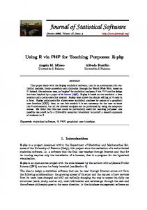
term in a document. English stopwords are removed from the matrix (it suffices to pass over TRUE to stopwords since the function looks up the language in each text document and loads the right stopwords automagically) R> crudeTDM (crudeTDMHighFreq Data(crudeTDM)[1:10, crudeTDMHighFreq] 10 x 3 sparse Matrix of class "dgCMatrix" oil opec kuwait 127 5 . . 144 12 15 . 191 2 . . 194 1 . . 211 1 . . 236 7 8 10 237 4 1 . 242 3 2 1 246 5 2 . 248 9 6 3 Another approach available in common text mining tools is finding associations for a given term, which is a further form of count-based evaluation methods. This is especially interesting when analyzing a text for a specific purpose, e.g., a business person could extract associations of the term “oil” from the Reuters articles. Technically we can realize this in R by computing correlations between terms. We have prepared a function findAssocs() which computes all associations for a given term and corlimit, that is the minimal correlation for being identified as valid associations. The example finds all associations for the term “oil” with at least 0.85 correlation in the termdocument matrix: R> findAssocs(crudeTDM, "oil", 0.85)

Journal of Statistical Software

29

saudi

month

sources

production

opec

mln

riyals

kuwait

report

budget

bpd

prices

billion

oil

market

nymex

indonesia

government

futures

economic

exchange

Figure 6: Visualization of the correlations within a term-document matrix. oil opec 1.00 0.87 Internally we compute the correlations between all terms in the term-document matrix and filter those out higher than the correlation threshold. Figure 6 shows a plot of the term-document matrix crudeTDM which visualizes the correlations over 0.5 between frequent (co-occurring at least 6 times) terms. Conceptually, those terms with high correlation to the given term oil can be interpreted as its valid associations. From the example we can see that oil is highly associated with opec, which is quite reasonable. As associations are based on the concept of similarities between objects, other similarity measures could be used. We use correlations between terms, but

30

Text Mining Infrastructure in R

theoretically we could use any well defined similarity function (confer to the discussion on the dissimilarity() function in the next section) for comparing terms and identifying similar ones. Thus the similarity measures may change but the idea of interpreting similar objects as associations is general.

5.2. Simple text clustering In this section we will discuss classical clustering algorithms applied to text documents. For this we combine our known acq and crude data sets to a single working set ws in order to use it as input for several simple clustering methods R> ws summary(ws) A text document collection with 70 text documents The metadata consists of 2 tag-value pairs and a data frame Available tags are: merge_date merger Available variables in the data frame are: MetaID

Hierarchical clustering Here we show hierarchical clustering (Johnson 1967; Hartigan 1975; Anderberg 1973; Hartigan 1972) with text documents. Clearly, the choice of the distance measure significantly influences the outcome of hierarchical clustering algorithms. Common similarity measures in text mining are Metric Distances, Cosine Measure, Pearson Correlation and Extended Jaccard Similarity (Strehl et al. 2000). We use the similarity measures offered by dist from package proxy (Meyer and Buchta 2007) in our tm package with a generic custom distance function dissimilarity() for term-document matrices. So we could easily use as distance measure the Cosine for our crude term-document matrix R> dissimilarity(crudeTDM, method = "cosine") Our dissimilarity function for text documents takes as input two text documents. Internally this is done by a reduction to two rows in a term-document matrix and applying our custom distance function. For example we could compute the Cosine dissimilarity between the first and the second document from our crude collection R> dissimilarity(crude[[1]], crude[[2]], "cosine") 127 144 0.4425716 In the following example we create a term-document matrix from our working set of 70 news articles (Data() accesses the slot holding the actual sparse matrix)

Journal of Statistical Software

31

100

crude crude crude crude crude crude crude crude acq crude acq acq acq acq acq acq acq acq acq acq acq acq acq acq acq acq acq crude acq acq acq acq acq acq acq acq acq acq acq crude crude acq acq acq acq acq acq acq acq acq acq acq crude acq acq acq acq acq acq acq acq crude crude crude crude acq crude crude acq crude

0

50

Height

150

200

250

Cluster Dendrogram

dist(wsTDM) hclust (*, "ward")

Figure 7: Dendrogram for hierarchical clustering. The labels show the original group names. R> wsTDM wsHClust wsKMeans wsReutersCluster cl_agreement(wsKMeans, as.cl_partition(wsReutersCluster), "diag") Cross-agreements using maximal co-classification rate: [,1] [1,] 0.7 which means that the k-means clustering results can recover about 70 percent of the human clustering. For a real-world example on text clustering for the tm package with several hundreds of documents confer to Karatzoglou and Feinerer (2007) who illustrate that text clustering with a decent amount of documents works reasonably well.

5.3. Simple text classification In contrast to clustering, where groups are unknown at the beginning, classification tries to put specific documents into groups known in advance. Nevertheless the same basic means can be used as in clustering, like bag-of-words representation as a way to formalize unstructured text. Typical real-world examples are spam classification of e-mails or classifying news articles into topics. In the following, we give two examples: first, a very simple classifier (k-nearest neighbor), and then a more advanced method (Support Vector Machines).

k-nearest neighbor classification Similar to our examples in the previous section we will reuse the term-document matrix representation, as we can easily access already existing methods for classification. A possible classification procedure is k-nearest neighbor classification implemented in the class (Venables and Ripley 2002) package. The following example shows a 1-nearest neighbor classification in a spam detection scenario. We use the Spambase database from the UCI Machine Learning Repository (Asuncion and Newman 2007) which consists of 4601 instances representing spam and nonspam e-mails. Technically this data set is a term-document matrix with a limited set of terms (in fact 57 terms with their frequency in each e-mail document). Thus we can easily bring text documents into this format by projecting our term-document matrices onto their 57 terms. We start with a training set with about 75 percent of the spam data set resulting in about 1360 spam and 2092 nonspam documents R> train trainCl test trueCl knnCl (nnTable sum(diag(nnTable))/nrow(test) [1] 0.7119234

Support vector machine classification Another typical, more sophisticated, classification method are support vector machines (Cristianini and Shawe-Taylor 2000). The following example shows an SVM classification based on methods from the kernlab package. We used the same training and test documents. Based on the training data and its classification we train a support vector machine: R> ksvmTrain svmCl (svmTable sum(diag(svmTable))/nrow(test) [1] 0.8772846 The results have improved over those in the last section (compare the improved cross-agreement) and prove the viability of support vector machines for classification. Though, we use a realisitic data set and gain rather good results, this approach is not competitive with available contemporary spam detection methods. The main reason is that spam detection nowadays encapsulates techniques far beyond analysing the corpus itself. Methods encompass mail format detection (e.g., HTML or ASCII text), black- (spam) and whitelists (ham), known spam IP addresses, distributed learning systems (several mail servers communicating their classifications), attachment analysis (like type and size), and social network analysis (web of trust approach). With the same approach as shown before, it is easy to perform classifications on any other form of text, like classifying news articles into predefined topics, using any available classifier as suggested by the task at hand.

5.4. Text clustering with string kernels This section covers string kernels, which are methods dealing with text directly, and not anymore with an intermediate representation like term-document matrices. Kernel-based clustering methods, like kernel k-means, use an implicit mapping of the input data into a high dimensional feature space defined by a kernel function k k(x, y) = hΦ(x), Φ(y)i , with the projection Φ : X → H from the input domain X to the feature space H. In other words this is a function returning the inner product hΦ(x), Φ(y)i between the images of two data points x, y in the feature space. All computational tasks can be performed in the feature space if one can find a formulation so that the data points only appear inside inner products. This is often referred to as the “kernel trick” (Sch¨olkopf and Smola 2002) and is computationally much simpler than explicitly projecting x and y into the feature space H. The main advantage is that the kernel computation is by far less computationally expensive than operating directly in the feature space. This allows one to work with high-dimensional spaces, including natural texts, typically consisting of several thousand term dimensions. String kernels (Lodhi et al. 2002; Shawe-Taylor and Cristianini 2004; Watkins 2000; Herbrich 2002) are defined as a similarity measure between two sequences of characters x and y. The generic form of string kernels is given by the equation X X k(x, y) = λs δs,t = nums (x)nums (y)λs , svx,tvy

s∈Σ∗

Journal of Statistical Software

35

where Σ∗ represents the set of all strings, nums (x) denotes the number of occurrences of s in x and λs is a weight or decay factor which can be chosen to be fixed for all substrings or can be set to a different value for each substring. This generic representation includes a large number of special cases, e.g., setting λs 6= 0 only for substrings that start and end with a white space character gives the “bag of words” kernel (Joachims 2002). Special cases are λs = 0 for all |s| > n, that is comparing all substrings of length less that n, often called full string kernel. The case λs = 0 for all |s| = 6 n is often referred to as string kernel. A further variation is the string subsequence kernel X kn (s, t) = hφu (s), φu (t)i u∈Σn

=

X X u∈Σn i:u=s[i]

=

X X

X

λl(i)

λl(j)

j:u=t[j]

X

λl(i)+l(j) ,

u∈Σn i:u=s[i] j:u=t[j]

where kn is the subsequence kernel function for strings up to the length n, s and t denote two strings from Σn , the set of all finite strings of length n, and |s| denotes the length of s. u is a subsequence of s, if there exist indices i = (i1 , . . . , i|u| ), with 1 ≤ i1 < · · · < i|u| ≤ |s|, such that uj = sij , for j = 1, . . . , |u|, or u = s[i] for short. λ ≤ 1 is a decay factor. A very nice property is that one can find a recursive formulation of the above kernel k00 (s, t) = 1, for all s, t, ki0 (s, t) = 0, if min(|s|, |t|) < i, ki (s, t) = 0, if min(|s|, |t|) < i, X 0 ki0 (sx, t) = λki0 (s, t) + ki−1 (s, t[1 : (j − 1)])λ|t|−j+2 , with i = 1, . . . , n − 1, j:tj =x

kn (sx, t) = kn (s, t) +

X

0 kn−1 (s, t[1 : (j − 1)])λ2 ,

j:tj =x

which can be used for dynamic programming aspects to speed up computation significantly. Further improvements for string kernel algorithms are specialized formulations using suffix trees (Vishwanathan and Smola 2004) and suffix arrays (Teo and Vishwanathan 2006). Several string kernels with above explained optimizations (dynamic programming) have been implemented in the kernlab package (Karatzoglou et al. 2004, 2006) and been used in Karatzoglou and Feinerer (2007). The interaction between tm and kernlab is easy and fully functional, as the string kernel clustering constructors can directly use the base classes from the tm classes. This proves that the S4 extension mechanism can be used effectively by passing only necessary information to external methods (i.e., the string kernel clustering constructors in this context) and still handle detailed meta information internally (i.e., the native text mining classes). The following examples show an application of spectral clustering (Ng et al. 2002; Dhillon et al. 2005), which is a non-linear clustering technique using string kernels. We create a string kernel for it R> stringkern stringCl table("String Kernel" = stringCl, Reuters = wsReutersCluster) Reuters String Kernel acq crude 1 46 1 2 4 19 This method yields the best results (the cross-agreement is 0.93) as we almost find the identical clustering as the Reuters employees did manually. This well performing method has been investigated by Karatzoglou and Feinerer (2007) and seems to be a generally viable method for text clustering.

6. Analysis of the R-devel 2006 mailing list This section shows the application of the tm package to perform an analysis of the R-devel mailing list (https://stat.ethz.ch/pipermail/r-devel/) newsgroup postings from 2006. We will both show to utilize metadata and the text corpora themselves. For the first we analyze author and topic relations whereas for the second we concentrate on investigating the e-mail contents and discriminative terms (e.g., match the e-mail subjects the actual content). The mailing list archive provides downloadable versions in gzipped mbox format. We downloaded the twelve archives from January until December 2006, unzipped them and concatenated them to a single mbox file 2006.txt for convenience. The mbox file holds 4583 postings with a file size of about 12 Megabyte. We start by converting the single mbox file to eml format, i.e., every newsgroup posting is stored in a single file in the directory 2006/. R> convertMboxEml("2006.txt", "2006/") Next, we construct a text document collection holding the newsgroup postings, using the default reader shipped for newsgroups (readNewsgroup()), and setting the language to American English. For the majority of postings this assumption is reasonable but we plan automatic language detection (Sibun and Reynar 1996) for future releases, e.g., by using n-grams (Cavnar and Trenkle 1994). So you can either provide a string (e.g., en_US) or a function returning a character vector (a function determining the language) to the language parameter. Next, we want the the postings immediately loaded into memory (load = TRUE)

Journal of Statistical Software

37

R> rdevel rdevel rdevel rdevel summary(rdevel) A text document collection with 4583 text documents The metadata consists of 2 tag-value pairs and a data frame Available tags are: create_date creator Available variables in the data frame are: MetaID We create a term-document matrix, activate stemming and remove stopwords. R> tdm authors authors sort(table(authors), decreasing = TRUE)[1:3] authors ripley at stats.ox.ac.uk (Prof Brian Ripley) 483 murdoch at stats.uwo.ca (Duncan Murdoch) 305 ggrothendieck at gmail.com (Gabor Grothendieck) 190 Next, we identify the three most active threads, i.e., those topics with most postings and replies. Similarly, we extract the thread name from the text document collection: R> headings headings (bigTopicsTable bigTopics ' + citations 0) + c