a complete MRF model, most of the âmassâ associated with the joint PDF will .... [3] Julian E. Besag, âOn the statistical analysis of dirty pictures,â Journal Of The Royal ... (a) D1 - aluminum wire mesh; (b) D15 - straw; (c) D20 - magnified French.
Texture Synthesis via a Non-parametric Markov Random Field Rupert Paget and Dennis Longstaff Department of Electrical and Computer Engineering, University of Queensland, and the Cooperative Research Centre for Sensor, Signal, and Information Processing QLD 4072 AUSTRALIA
ABSTRACT In this paper we present a non-causal non-parametric multiscale Markov random field (MRF) texture model that is capable of synthesising a wide variety of textures. The textures that this model is capable of synthesising vary from the highly structured to the stochastic type and include those found in the Brodatz album of textures. The texture model uses Parzen estimation to estimate the conditional probability density function that defines the MRF. For texture synthesis we introduce a novel multiscale approach. We show that these two facets of the model give the ability to model textures requiring large neighbourhood systems to incorporate high order statistical properties of the texture.
1
INTRODUCTION
Texture is the visual characteristics of an image segment that identifies it as belonging to a unique class. A class might be associated with a particular physical interpretation such as: grass, hair, water, or sand. Examples of such textures are shown in Brodatz album of textures [5]. In image processing, texture can be defined in terms of spatial pixel value interactions within a digital image. The aim of texture analysis is to model these spatial interactions. If the spatial interactions can be modelled for a particular texture, then it becomes possible to segment and delineate that particular texture from the rest of the image via the model. The segmented area can then be classified as belonging to the same class as that particular texture. The difficulty lies in finding a model which is unique to the particular texture, for without this there is the potential for misclassification of hitherto unknown textures. Texture analysis to date has been primarily concerned with just the first and second order statistical properties of texture. Texture models that have used only the first and second order statistical properties have only been able to synthesis the basic of textures for which they model. To synthesis a texture from its model means the model has to hold the complete characteristics of that texture. To synthesis complex textures like the Brodatz textures higher order statistical properties must be used. One model that is capable of modelling these properties is the Markov random field (MRF) model. Parametric versions of the MRF model are prohibitive for modelling the high order properties, therefore we present a non-parametric MRF model that can model these high order statistical properties. The model presented in this paper would be unsuitable for image compression or fast texture synthesis, for such purposes a parametric model would be required. However, as the texture model presented in this paper is capable accurately synthesising a wide variety of textures, it represents the basis of a complete texture model. Such a model would be suitable for segmenting an image into its various texture types and classifying the segmented regions accordingly.
2
MARKOV RANDOM FIELD TEXTURE MODEL
Markov random field (MRF) models have been used in image restoration [11], region segmentation [10] and texture synthesis [6]. The property of a MRF is that: a variable Xs on a lattice S = {s = (i, j) : 0 ≤ i, j < N } can have its value xs set to any value, but the probability of Xs = xs is conditional upon the values xr at its “neighbouring” sites r ∈ Gs . A local conditional probability density function (LCPDF) defined over these neighbouring sites r ∈ Gs determines how the variable Xs is set. The neighbourhood system G = {Gs , s ∈ S} and the LCPDF defined with respect to G and written P (Xs = xs |Xr = xr , r ∈ Gs ) s ∈ S
(1)
defines the MRF [1]. To model an image as a MRF, consider each pixel in the image as a site on a lattice, and the grey scale value associated with the pixel the value of that site. If the image is all of one texture, then the LCPDF derived from the image is the model that defines the texture. The uniqueness of the model can be tested by synthesising a texture via the LCPDF. If the model is unique to the texture then it is that texture which will most likely be synthesised.
(a)
(b)
(c)
Figure 1: Neighbourhoods. (a) The first order neighbourhood (c = 1) or “nearest-neighbour” neighbourhood for the site s = (i, j) = ‘•’ and r = (k, l) ∈ Gs = ‘◦’; (b) second order neighbourhood (c = 2); (c) eighth order neighbourhood (c = 8). The neighbourhood systems employed in this paper are the same as in [9] and [11] for which the neighbourhood system G c = {Gsc , s = (i, j) ∈ S} is defined as Gsc = {r = (k, l) ∈ S : 0 < (k − i)2 + (l − j)2 ≤ c}
(2)
where c refers to the order of the neighbourhood system. Neighbourhood systems for c = 1, 2 and 8 are shown in Fig.1
3
NON-PARAMETRIC MRF MODEL
Given an image of a homogeneous texture, and a predefined neighbourhood system, a nonparametric estimate of the LCPDF can be obtained by creating a multi-dimensional histogram with respect to the neighbourhood system. As an example lets choose a small neighbourhood system, G = {Gs=(i,j) } such that Gs=(i,j) = {r = (i − 1, j), t = (i, j − 1)}. Define a 3-dimensional histogram with dimensions (u, v, w) and a variable Y(u,v,w) = 0. The 3dimensional histogram of the image is then formed by raster scanning all the pixels in the image s ∈ S for which the neighbourhood Gs ⊂ S, and incrementing the variable Y(u,v,w) at the position (u = xs , v = xr , w = xt ). Since every site s ∈ S for which the specified neighbourhood Gs ⊂ S is used in creating the 3-dimensional histogram, the data obtained from the image is not independent and identically distributed (i.i.d.). However this technique for building the multi-dimensional histogram uses the same non i.i.d. data that is used in the “pseudo-likelihood” estimate for the LCPDF
proposed by Besag [2]. Besag [4] showed that this was an efficient technique for estimating the LCPDF for a Gaussian MRF. Geman and Graffigne [12] also proved that for a LCPDF defined over an equivalent Gibbs random field, the estimate found by the pseudo-likelihood technique converged to the true LCPDF with a probability one as the field increased to infinity. On this evidence we justify our use of non i.i.d. data for estimating our non-parametric version of the LCPDF. The LCPDF is obtained by performing density estimation on the multi-dimensional histogram. If we want to be very naive about the form the LCPDF, the best option is to use a non-parametric density estimator. The most common non-parametric density estimator is the Parzen-window density estimator [8].
4
PARZEN WINDOW DENSITY ESTIMATOR
The Parzen-window density estimator has the effect of smoothing each sample data point in the multi-dimensional histogram over a larger area, possibly in the shape of a multi-variate Gaussian surface. To estimate the true density function f from a sample of n real observations Y1 , . . . , Yn in the d-dimensional histogram, the estimate density function fˆ is given by � � n 1 1 X (y − Y ) K fˆ(y) = k nhd k=1 h
(3)
The shape of the smoothing is defined by the kernel function K. The size of the kernel is defined by the window parameter h. If h is too small, random error effects remain dominant, and no generalisations can be deduced. If h is too large, then all the useful information is lost in a “blur.” If the kernel function K(y) is chosen to be a standard multivariate normal density function 1 1 exp(− y T y), (4) K(y) = d/2 2 (2π) then from Silverman [14, p 85] an optimal window parameter hopt is hopt = σ
�
4 n(2d + 1)
�1/(d+4)
(5)
where σ 2 is the the average marginal variance. In our case the marginal variance is the same in each dimension and therefore σ 2 equals the variance associate with the one-dimensional histogram. Note, the formula for hopt given by Silverman [14] was derived with respect to assumptions made about the true density function f , one being that f is a standard multivariate normal density function.
5
TEXTURE SYNTHESIS
A texture can be synthesised from a MRF model via a method known as stochastic relaxation (SR). SR iteratively generates a succession of images which converge to an image with a probability given by the joint probability distribution function (PDF) of the MRF [11]. For a complete MRF model, most of the “mass” associated with the joint PDF will cover those images most like the texture being modeled. Therefore a texture synthesised via SR using a complete MRF model should be similar to the original texture. SR generates the sequence of images by replicating all but one random pixel value from one image to the next. The pixel value that is not replicated is replaced by a pixel value selected with respect to the LCPDF. Two well known SR algorithms are the Metropolis algorithm and the Gibbs sampler. These algorithms appear in [7] [9] and [11].
A deterministic relaxation algorithm was introduced by Besag [3] as the “iterative conditional modes” (ICM) algorithm. In this case for the pixel whose value is to be updated, the ICM algorithm returns the mode of the LCPDF. The ICM algorithm will most likely find equilibrium at a local maximum of the joint PDF. A realisation of an image at a local maximum should be all that is required to produce a reasonably similar texture.
6
MULTISCALE RELAXATION
The basic concept of multiscale relaxation of an MRF is to relax the field at various “resolutions.” The advantage is that some characteristics of a field are more prominent at some resolutions than at others. For example high frequency characteristics are prominent at high resolutions but are hidden at low resolutions. In contrast, low frequency characteristics are easier relaxed at low resolutions [13]. l=2
6 decreasing image resolution
l=1
6 increasing grid level
l=0
Figure 2: Possible grid organisation for multiscale modelling of a MRF. A small portion of three levels of a 2:1 multigrid hierarchy is shown. Only connections representing nearest-neighbour interactions are included.
The multiscale model can be best described through the use of a multigrid representation of the field as shown in Figure 2. The grid at level l = 0 represents the original image, where each intersection point ‘•’ is a site s ∈ S. The multigrid displayed in Figure 2 shows the connections involved in a decimation procedure for multiscale relaxation [13]. The algorithm starts at the lowest resolution and uses deterministic relaxation (ICM). Once an equilibrium state has been reached by the ICM, the image is propagated down to the the next level where it undergoes further relaxation. In our algorithm we also use an energy function that allows for the information transferred down from the previous level to be better incorporated into the estimation of the LCPDF.
7
ENERGY FUNCTION
Define an energy es at site s ∈ S on the same lattice as the image to undergo multiscale relaxation. Consider the relaxation of an image at level l. Before the relaxation starts, initialize es = 1 if s ∈ grid at previous level (l + 1), otherwise es = 0. After the pixel value xs has been updated the energy es at the same site s is updated to es =
1+
P
r∈Gs er
|Gs |
(6)
where er is the energy at the site r. If es > 1 equate es = 1. At each iteration when estimating the LCPDF via the Parzen density estimator use the modified form of (y − Yk ) in equation (3). s (y − Yk ) =
X
r∈Gs
(yr − Ykr )2 .e2r
(7)
The multiplication of e2r in the formula represents a “confidence” in using that site to calculate the LCPDF. Initially only those sites who have had their values relaxed at the previous level (l + 1) are used in the LCPDF, but as the iterations progress more sites gain a degree of “confidence.” When all es = 1 at level l it becomes time to move to the next level (l − 1) and begin again.
8
RESULTS
The textures displayed in Figure 3 were synthesised from the corresponding Brodatz texture. The synthesis algorithm employed was a multiscale ICM texture synthesis algorithm with the energy function described in section 7 used to determine the LCPDF. The texture model was obtained from a 128 × 128 image, and the synthesis was performed on a 256 × 256 image. This was done to confirm that the characteristics of the texture were indeed captured, and it was these captured characteristics that allowed the algorithm to synthesis the texture over a larger area. Therefore we believe that the non-causal non-parametric multiscale Markov random field texture model forms a highly representative model of the texture.
References [1] Julian E. Besag, “Spatial interaction and the statistical analysis of lattice systems,” Journal of the Royal Statistical Society, series B, vol. 36, pp. 192–326, 1974. [2] Julian E. Besag, “Statistical analysis of non–lattice data,” Statistician, vol. 24, pp. 179–195, 1975. [3] Julian E. Besag, “On the statistical analysis of dirty pictures,” Journal Of The Royal Statistical Society, vol. B–48, pp. 259–302, 1986. [4] Julian E. Besag and P. A. P. Moran, “Efficiency of pseudo–likelihood estimation for simple Gaussian fields,” Biometrika, vol. 64, pp. 616–618, 1977. [5] P. Brodatz, Textures – a photographic album for artists and designers, Dover Publications Inc., New York, 1966. [6] G. C. Cross and A. K. Jain, “Markov random field texture models,” IEEE Transactions on Pattern Analysis and Machine Intelligence, vol. 5, pp. 25–39, 1983. [7] Richard C. Dubes and Anil K. Jain, “Random field models in image analysis,” Journal of Applied Statistics, vol. 16, no. 2, pp. 131–164, 1989. [8] Richard O. Duda and Peter E. Hart, Pattern Classification and Scene Analysis, John Wiley, Stanford Reseach Institute, Menlo Park, California, 1973. [9] D. Geman, “Random fields and inverse problems in imaging,” in Lecture Notes in Mathematics, vol. 1427, pp. 113–193. Springer–Verlag, 1991. [10] Donald Geman, Stuart Geman, Christine Graffigne, and Ping Dong, “Boundary detection by constrained optimization,” IEEE Transactions on Pattern Analysis and Machine Intelligence, vol. 12, no. 7, pp. 609–628, 1990. [11] Stuart Geman and Donald Geman, “Stochastic relaxation, Gibbs distributions, and the Bayesian restoration of images,” IEEE Transactions on Pattern Analysis and Machine Intelligence, vol. 6, no. 6, pp. 721–741, 1984.
(a)
(a.1)
(a.2)
(b)
(b.1)
(b.2)
(c)
(c.1)
(c.2)
(d)
(d.1)
(d.2)
Figure 3: Brodatz textures: (a) D1 - aluminum wire mesh; (b) D15 - straw; (c) D20 - magnified French canvas; (d) D103 - loose burlap; (?.1) synthesised textures of the corresponding Brodatz texture - using neighbourhood order (c=8); (?.2) synthesised textures - using neighbourhood order (c=18).
[12] S. Geman and C. Graffigne, “Markov random field image models and their applications to computer vision,” Proceedings of the International Congress of Mathematicians, pp. 1496–1517, 1986. [13] Basilis Gidas, “A renormalization group approach to image processing problems,” IEEE Transactions on Pattern Analysis and Machine Intelligence, vol. 11, no. 2, pp. 164–180, 1989. [14] B. W. Silverman, Density estimation for statistics and data analysis, Chapman and Hall, London, 1986.