Imperial/TP/98–99/13.
arXiv:gr-qc/9811078v3 1 Mar 1999
The action operator for continuous-time histories
K. Savvidou1 Theoretical Physics Group Blackett Laboratory Imperial College of Science, Technology & Medicine London SW7 2BZ, U.K. November 1998
Abstract We define the action operator for the consistent histories formalism, as the quantum analogue of the classical action functional, for the simple harmonic oscillator case. We conclude that the action operator is the generator of time transformations, and is associated with the two types of time-evolution of the standard quantum theory: the wave-packet reduction and the unitary time-evolution. We construct the corresponding classical histories and demonstrate the relevance with the quantum histories. Finally, we show the relation of the action operator to the decoherence functional.
1
e-mail:
[email protected].
1
Introduction
One of the basic elements in the consistent histories formalism is the idea of a ‘homogeneous history’. This is a time-ordered sequence of propositions about the system and, in the original approaches to the formalism, is represented by a class operator C˜ C˜ := U(t0 , t1 )αt1 U(t1 , t2 )αt2 ...U(tn−1 , tn )αtn U(tn , t0 )
(1.1)
where αti is a single-time projection operator representing a property of the i ′ system at time ti , and U(t, t′ ) = e− h¯ H(t−t ) is the unitary time evolution operator. [4, 5, 16, 17] In the ‘History Projection Operator’ (HPO) approach developed by Isham and collaborators [1, 2, 3, 14], a homogeneous history “αt1 is true at time t1 and αt2 is true at time t2 ... and αtn is true at time tn ” is represented by a projection operator α, defined as the tensor product of projection operators α := αt1 ⊗αt2 ⊗...⊗αtn on the n-fold tensor product of copies of the standard Hilbert space Vn := Ht1 ⊗ Ht2 ⊗ ... ⊗ Htn . This approach re-establishes the logical nature of propositions about a physical system since these projection operators (and their disjunctions) represent a type of temporal quantum logic. Most discussions of the consistent-histories formalism have involved histories defined at a finite set of time points. However, it is important to extend this to include a continuous time variable (especially for potential applications to quantum field theory), and in order to construct continuoustime histories on the continuous tensor product of copies of the Hilbert space Vcts := ⊗Ht , Isham and Linden defined the History Group [2] as an analogue of the canonical group of normal quantum theory. This group plays a crucial role in the physical interpretation of the theory: the spectral projectors of the generators of its Lie algebra represent history propositions about the system. For the example of a non-relativistic point particle moving on a line, the history group was defined as a generalised Weyl group with Lie algebra [ xt , xt′ ] = 0 [ pt , pt′ ] = 0 hτ δ(t − t′ ) [ xt , pt′ ] = i¯
(1.2) (1.3) (1.4)
where −∞ < t, t′ < +∞ and τ is a constant with dimensions of time. It is important to emphasise that the generators of the history algebra xt and 1
pt , t ∈ R, are Schr¨odinger-picture operators. After being properly smeared, they correspond (actually, their spectral projectors), to propositions about the time-averaged values of the position and the momentum of the system respectively. The evident resemblance of the history algebra to the algebra of a quantum field theory meant that the one-dimensional quantum mechanics history theory could be treated mathematically in some respects as a 1 + 1 dimension quantum field theory. In a previous paper [1], the requirement of the existence of the Hamiltonian operator H which represents propositions about the time-averaged values of the energy of the system—in particular, for the example of a simple harmonic oscillator in one dimension—together with the explicit relation between the Hamiltonian and the creation and annihilation operators, selected uniquely a Fock space as the representation space of the history algebra [1.21.4] on the history space Vn . We shall return to this representation in more detail shortly. The history algebra generators xt and pt can be seen heuristically as operators, (actually they are operator-valued distributions on Vn ), that for each time label t, are defined on the Hilbert space Ht . The question then arises if, and how, these Schr¨odinger-picture objects with different time labels are related: in particular, is there a transformation law ‘from one Hilbert space to another’ ? One anticipates that the analogue of this question in the context of a histories treatment of a relativistic quantum field theory would be crucial to showing the Poincar´e invariance of the system. In the Hamilton-Jacobi formulation of Classical Mechanics, it is the action functional that plays the role of the generator of a canonical transformation of the system from one time to another. Indeed, the Hamilton-Jacobi functional S, evaluated for the realised path of the system—i.e., for a solution of the classical equations of motion, under some initial conditions—is the generating function of a canonical transformation, which transforms the system variables position x and momentum p from an initial time t = 0 to another time t. It is therefore natural to investigate whether a quantum analogue of the action functional exists for the HPO theory. Indeed, in [1] where we explored the quantum field theory case for the continuous-time histories, we were not able to show the manifest covariance of the theory under the ‘external’ Poincar´e group. However, we did not consider the action as an operator; the main goal of the present paper is to enhance the theory in this direction so as to have a clearer view of the time-transformation issue. This will ultimately allow us to re-address the 2
problem of the Poincar´e covariance of the quantum field theory [?] In what follows, we first prove the existence of the action operator Sκ , using the same type of quantum field theory methods that were used to prove the existence of the Hamiltonian operator Hκ [1]. We will show that, constructed as a quantum analogue of the classical action functional, Sκ does indeed act as a generator of time-transformations in the HPO theory. Furthermore—and more speculatively—this is arguably related to the two laws of time-evolution in standard quantum theory: namely, wave-packet reduction and the unitary time-evolution between measurements. A comparison with the classical theory case seems appropriate at this point, and thus, in Sections 3 and 4, we present a classical analogue of the HPO, where the continuous-time classical histories can be seen to be an analogue of the continuous-time quantum histories. In Section 5, we further exploit the classical analogy to discuss the ‘classical’ behaviour of the history quantum scheme. In particular, we expect the action operator to be involved in some way with the dynamics of the theory. To this end, we show how it appears in the expression for the decoherence functional expression, with operators acting on coherent states, as used earlier by Isham and Linden [2].
2
The action operator defined
In the generalised consistent histories theory by Gell-Mann and Hartle [4, 5] and others, a homogeneous history α is a time-ordered sequence of propositions about the system, and is represented by a class operator C˜ C˜ := U(t0 , t1 )αt1 U(t1 , t2 )αt2 ...U(tn−1 , tn )αtn U(tn , t0 )
(2.1)
where αti is a single-time projection operator representing a proposition about the system at time ti . If a particular history α belongs to a consistent set, then the probability for the history to be realised is Prob(α) = trH C˜α† ρt0 C˜α
(2.2)
where ρt0 is the density matrix of the initial state. Deciding whether or not a particular set of histories is consistent involves evaluating the decoherence functional d(α, β) := trH C˜α† ρt0 C˜β (2.3) 3
which is a complex-valued function of a pair of histories α and β. In particular, if α and β are disjoint propositions belonging to a consistent set, then they satisfy the ‘decoherence’ condition d(α, β) = 0
(2.4)
We note that, as a product of projectors, the class operator C˜α is generally not itself a projector, and hence the temporal logic structure of quantum mechanics is lost. This is remedied in the HPO theory, in which the history proposition “αt1 is true at time t1 and αt2 is true at time t2 ... and αtn is true at time tn ” is represented by the tensor product α := αt1 ⊗ αt2 ⊗ ... ⊗ αtn [14]. This is a genuine projection operator on the n-fold tensor product Vn := Ht1 ⊗ Ht2 ⊗ ... ⊗ Htn . Each constituent proposition αt , labelled by the time parameter t, is defined on a copy of the standard quantum theory Hilbert space, with the same t-label Ht . This is a straightforward idea for a discrete set of times (t1 , t2 , . . . , tn ) but, for reasons given in the Introduction, it is important to extend these ideas to continuous-time histories which are to be defined on some sort of continuous tensor product of copies of the Hilbert space Vcts := ⊗Ht . A key technical tool is the history group, constructed as an analogue of the canonical group [16] of normal quantum theory. For a particle moving in one dimension, the standard canonical commutation relation [ x, p ] = i¯ h
(2.5)
is replaced by the ‘history algebra’ [ xt , xt′ ] = 0 [ pt , pt′ ] = 0 hτ δ(t − t′ ) [ xt , pt′ ] = i¯
(2.6) (2.7) (2.8)
where −∞ < t, t′ < +∞. The constant τ has dimensions of time [15] and, in what follows, for convenience we shall choose units in which τ = 1 . These operators are written in the Schr¨odinger picture: t labels the Hilbert space— it is not the time parameter that appears in the Heisenberg picture for normal quantum theory. To be mathematically precise, the eqs. (2.6—2.7) must be smeared [ xf , xg ] = 0 [ pf , pg ] = 0
(2.9) (2.10)
[ xf , pg ] = i¯ h
Z
4
+∞
−∞
f (t)g(t)dt
(2.11)
where f and g belong to some appropriate subset of the space L2 (R, dt) of square integrable functions on R. The evident resemblance of the above with the canonical commutation algebra of a quantum field theory in 1 + 1 dimensions, leads to the treatment of the history algebra using mathematical ideas drawn from the former. In particular, a unique representation of the history algebra can be selected by the requirement that a representation of the (analogue of the) Hamiltonian operator exists [13]: physically, this operator represents history propositions about the time-averaged values of the energy. In previous work [1], we explored the familiar example of a simple harmonic oscillator in one dimension. In this case, the history algebra is extended to include the commutators i¯ h [ Hκ , xf ] = − pκf (2.12) m [ Hκ , pf ] = i¯ hω 2xκf (2.13) (2.14) [ Hκ , Hκ ′ ] = 0 ∞ where Hκ is the time-averaged history energy operator Hκ := −∞ κ(t)Ht dt. The smearing function κ(t) belongs to some subset of the space L2 (R, dt), in general not the same as the subset on which the test functions of the xt and pt are defined. The specific choice of test functions is partly determined by the physical situations to which the formalism is to be applied. The Fock representation of the history algebra, is based on the definition of the ‘annihilation’ operator
R
bt :=
r
s
mω 1 xt + i pt 2¯ h 2mω¯ h
(2.15)
with commutation relations [ bt , bt′ ] = 0 [ bt , b†t′ ] = δ(t − t′ )
(2.16) (2.17)
and is uniquely selected by the requirement that the time-averaged Hamiltonian operator exists in this representation; heuristically, Ht is connected with the operator b† by the expression Ht = h ¯ ωb†t bt . In the Hamiltonian formalism for a classical system, the action functional is defined as Z +∞ Scl := (pq˙ − H)dt (2.18) −∞
5
where q is the position, p is the momentum and H the Hamiltonian of the system. Following the same line of thought as for the definition of the Hamiltonian algebra, we want to find a representation of the history algebra in which their exists a one-parameter family of operators St —or better their smeared form Sλ,κ . Heuristically we have St := (pt x˙ t − Ht ) Sλ,κ :=
Z
+∞
−∞
(2.19)
(λ(t)pt x˙ t − κ(t)Ht )dt
(2.20)
where Sλ,κ is the smeared action operator with smearing functions λ(t), κ(t). In order to discuss the existence of an operator Sλ,κ we note that, if this operator exists, the Hamiltonian algebra eqs. (2.12 — 2.14), would be augmented in the form pκf [ Sλ,κ , xf ] = i¯ h(x d (λf ) + ) (2.21) dt m [ Sλ,κ , pf ] = i¯ h(pλf + mωxκf ) (2.22) Z ∞ i¯ h ˙ p˙2t )dt (κ′ (t)λ(t) (2.23) hH d (λκ′ ) − [Sλ,κ , Hκ′ ] = i¯ dt m −∞ ′ hH d (λκ′ ) − [ Sλ,κ , Sλ,κ ] = i¯ hH d (λ′ κ) − i¯ dt
i¯ h
dt
p˙2t ˙ )dt ([(κ(t)λ˙′ (t)) − (κ′ (t)λ(t))] m −∞
Z
∞
(2.24)
Although we have defined the action operator in a general smeared form, in what follows we will mainly employ only the case λ(t) = 1 and κ(t) = 1 that accords with the expression for the classical action functional. This choice of smearing functions poses no technical problems restrictions, provided we keep to the requirement that the smearing functions for the position and momentum operators are square-integrable functions. In particular, the products of the smearing functions f and g in eqs (2.21—2.24) with the test functions λ(t) = 1 and κ(t) = 1 with, are still square-integrable. The existence of the action operator in HPO. We now examine whether the action operator actually exists in the Fock representation of the history algebra employed in our earlier work[1]. Henceforward we choose λ(t) = 1. Then the formal commutation relations are Sκ :=
Z
+∞ −∞
6
(pt x˙ t − κ(t)Ht )dt
(2.25)
pκf ) m [ Sκ , pf ] = i¯ h(pf + mωxκf ) hHκ˙ ′ [ Sκ , Hκ′ ] = i¯ hHκ˙ − i¯ hHκ˙ ′ [ Sκ , Sκ′ ] = i¯ [ Sκ , xf ] = i¯ h(xf˙ +
(2.26) (2.27) (2.28) (2.29)
i
A key observation is that if the operators e h¯ Sκ existed they would produce the history algebra automorphism i
i
e h¯ Sκ bt e− h¯ Sκ = e−iω or, in the more rigorous smeared form i
R t+s t
d κ(t+s′ )ds′ +s dt
bt
i
e h¯ Sκ bf e− h¯ Sκ = bΣs f
(2.30)
(2.31)
where the unitary operator Σs is defined on L2 (R) by −iω
(Σs ψ)(t) := e
R t+s t
κ(t+s′ )ds′
ψ(t + s).
(2.32)
However, an important property of the Fock construction states that when there exists a unitary operator eisA acting on L2 (R), there exists a unitary operator Γ(eisA ) that acts on the exponential Fock space2 F (L2 (R)) in such way that −1 Γ(eisA )b†f Γ(eisA ) = b† eisA f (2.33) then the operator dΓ(A) on F (L2(R)) can also be defined as Γ(eisA ) = eisdΓ(A)
(2.34)
in terms of A, a self-adjoint operator that acts on L2 (R). In particular, it follows that the representation of the history algebra on the Fock space F (L2(R)) carries a (weakly continuous) representation of the one-parameter i family of unitary operators s 7→ e h¯ sSκ = Γ(Σs ). Therefore, the generator Sκ also exists on F (L2 (R)) and S = dΓ(−¯ hσκ ) where σκ is a self-adjoint operator that acts on L2 (R) and is defined as !
d ψ(t). σκ ψ(t) := −ωκ(t) − i dt
(2.35)
n A general expression for a Fock space is eH = ⊕∞ n=0 (⊗n H) where H is called the base H Hilbert space of the Fock space e . 2
7
In what follows, we will restrict our attention to the particular case κ(t) = 1 for the simple harmonic oscillator action operator S S :=
Z
+∞
−∞
(pt x˙ t − Ht )dt.
(2.36)
The Liouville operator definition. The first term of the action operator eq. (2.36) is identical to the kinematical part of the classical action functional eq. ( 2.18 ). For reasons that will become apparent later, we write Sκ as the difference between two operators: the Liouville operator and the Hamiltonian operator. The Liouville operator is formally written as V :=
Z
∞
−∞
(pt q˙t )dt
(2.37)
where Sκ = V − H κ
(2.38)
We prove the existence of V on F (L2(R)) using the same technique as before. Namely, we can see at once that the history algebra automorphism i
i
e h¯ sV bf e− h¯ sV = bBs f
(2.39)
is unitarily implementable. Here, the unitary operator Bs , s ∈ R, acting on L2 (R) is defined by d
(Bs f )(t) := es dt f (t) = eisD f (t) = f (t + s)
(2.40)
where D := −i dtd . The Liouville operator V has some interesting commutation relations with the generators of the history algebra: [ V, xf ] [ V, pf ] [ V, Hκ ] [ V, Sκ ] [ V, H ] [ V, S ] where we have defined H :=
R∞
−∞
= = = = = =
Ht dt. 8
−i¯ hxf˙ −i¯ hpf˙ −i¯ hHκ˙ i¯ hHκ˙ 0 0
(2.41) (2.42) (2.43) (2.44) (2.45) (2.46)
We notice that V transforms, for example, bt from one time t—that refers to the Hilbert space Ht —to another time t + s, that refers to Ht+s . More precisely, V transforms the support of the operator-valued distribution bt from t to t + s: i i e h¯ sV bf e− h¯ sV = bfs (2.47) where fs (t) := f (s + t). We shall return to the significance of this later. The Fourier-transformed ‘n-particle’ history propositions. An interesting family of history propositions emerges from the representation space F [L2 (R, dt)], acting on the δ-function normalised basis of states |0i, |t1 i := b†t1 |0i , |t1 , t2 i := b†t1 b†t2 |0i etc; or, in smeared form, |φi := b†φ |0i etc. The projection operator |tiht| corresponds to the history proposition ‘there is a unit energy h ¯ ω concentrated at the time point t’. The physical interpretation for this family of propositions, was deduced from the action of the Hamiltonian operator on the family of |ti states: Ht |0i = 0 Ht |t1 i = h ¯ ωδ(t − t1 )|t1 i Ht |t1 , t2 i = h ¯ ω[δ(t − t1 ) + δ(t − t2 )]|t1 , t2 i .. .
(2.48) (2.49) (2.50)
To study the behaviour of the S operator, a particularly useful basis for F [L2 (R, dt)] is the Fourier-transforms of the |ti-states. Indeed, if we consider the Fourier transformations |νi = |ν1 , ν2 i = bν = b†ν =
Z
+∞
−∞ Z +∞
−∞ Z +∞
−∞ Z +∞ −∞
eiνt b†t |0idt
(2.51)
eiν1 t1 eiν2 t2 b†t1 b†t2 |0idt1 dt2
(2.52)
eiνt bt dt
(2.53)
e−iνt b†t dt
(2.54)
the Fourier transformed |νi- states are defined by |νi := b†ν |0i, |ν1, ν2 i := b†ν1 b†ν2 |0i etc. The eigenvectors of the operator S are calculated to be S|0i = 0
(2.55) 9
S|νi = h ¯ (ν − ω)|νi S|ν1 , ν2 i = h ¯ [(ν1 − ω) + (ν2 − ω)]|ν1, ν2 i .. .
(2.56) (2.57)
i
and we note in particular that e h¯ sS |0i = |0i. The |νi-states are also eigenstates of the Hamiltonian operator: H|0i = 0 H|νi = h ¯ ω|νi H|ν1 , ν2 i = 2¯ hω|ν1, ν2 i .. .
(2.58) (2.59) (2.60)
∞ Again, as for the case of the |ti- states, for the special case of H := −∞ Ht dt, and for the simple harmonic oscillator example, we see how the integer-spaced spectrum of the standard quantum field theory appears in the HPO theory. The |νihν| history propositions give the spectrum of the action operator and they have an interesting connection with the |tiht| propositions.
R
2.1
The Velocity operator
In [1], we emphasised the existence of the operator x˙ t := dtd xt , that corresponds to history propositions about the velocity of the system. The velocity operator is better defined in its smeared form using the familiar quantum field theory procedure x˙ f = −xf˙ (2.61) In analogy with quantum field theory, this requires the function f to be differentiable and to ‘vanishes at infinity’ so that the implicit integration by parts in eq (2.61) is valid. We note that, in this HPO theory, the velocity operator commutes with the position [ xt , x˙ t′ ] = 0,
(2.62)
and therefore there exist history propositions about the position and the velocity at the same time. Furthermore, the existence of the Liouville operator in the HPO scheme, allows an interesting comparison between the velocity x˙ f and the momentum pf operators: namely, the momentum operator is defined by the history 10
commutation relation of the position with the Hamiltonian, while we can define the velocity operator from the history commutation relation of the position with the Liouville operator: pf [ xf , H ] = i¯ h (2.63) m [ xf , V ] = i¯ hx˙ f (2.64) These relations signify the different nature of the momentum pf from the velocity x˙ f concerning the dynamical behaviour of the momentum (related to the Hamiltonian operator), as opposed to the kinematical behaviour of the velocity (related to the Liouville operator).
2.2
The Heisenberg picture
In standard quantum theory, a Heisenberg-picture operator A(s) is defined as i i (2.65) AH (s) := e h¯ sH Ae− h¯ sH In particular, for the case of a simple harmonic oscillator, the equation of motion is d2 x(s) + ω 2 x(s) = 0 (2.66) ds2 from which we obtain the solution 1 sin(sω)p mω p(s) = −mω sin(sω)x + cos(sω)p x(s) = cos(sω)x +
(2.67) (2.68)
where we have used the classical equation p := m
dx(s) ds s=0
(2.69)
The commutation relations between these operators is [ x(s1 ), x(s2 ) ] =
i¯ h sin[ω(s1 − s2 )] mω
(2.70)
In formulating a history analogue of the Heisenberg picture [1], we adopted a ‘time-averaged’ Heisenberg picture defined by xκ,t := ei/¯hHκ xt e−i/¯hHκ = cos[ωκ(t)]xt + 11
1 sin[ωκ(t)]pt mω
(2.71)
for suitable test functions κ. The analogue of the equations of motion is the functional differential equation δ 2 xκ,t + δ(t − s1 )δ(t − s2 )ω 2 xκ,t = 0 δκ(s1 )δκ(s2 ) and δ(t − s)pt = m
δxκ,t δκ(s) κ=0
(2.72)
(2.73)
is the history analogue of the classical equation p := m dx(s) . ds s=0 We noted then that the Heisenberg-picture in an HPO theory involves two time labels: an ‘external’ label t—that specifies the time the proposition is asserted—and an ‘internal’ label s that, for a fixed time t, is the time parameter of the Heisenberg picture associated with the copy Ht of the standard Hilbert space. Using our new results, the two labels appear naturally in a new version of the Heisenberg picture: they are related to the groups that produce the two types of time transformations. In addition, the analogy with the classical expressions is regained. To see this explicitly, we define a Heisenberg picture analogue of xt as i
i
xκ,t,s : = e h¯ sHκ xt e− h¯ sHκ
pκ,t,s
1 = cos[ωsκ(t)]xt + sin[ωsκ(t)]pt mω i i : = e h¯ sHκ pt e− h¯ sHκ = −mω sin[ωsκ(t)]xt + cos[ωsκ(t)]pt
(2.74)
(2.75)
The commutation relations for these operators are i¯ h sin[ωκ(s′ − s)]δ(t − t′ ) (2.76) mω i h κ′ 1 ′ sin[sωκ(t)]p˙t − pκ,t,s (2.77) h cos[sωκ(t)]x˙t + [ xκ,t (s), Sκ ] = i¯ mω m h i ′ h cos[sωκ(t)]p˙t − mω sin[sωκ(t)]x˙t + κ′ (t)xκ,t,s (2.78) [ pκ,t (s), Sκ ] = i¯
[ xκ,t (s), xκ′ ,t′ (s′ ) ] =
and from these commutators we obtain the HPO analogue of the equations of motion d2 xκ,t,s + ω 2κ(t)2 xκ,t,s = 0 (2.79) 2 ds 12
We notice the strong resemblance with standard quantum theory; for the case κ(t) = 1, the classical expressions are fully recovered. In the HPO formalism, the Heisenberg picture objects appear time averaged with respect to the ‘external’ time label t. On the other hand, the ‘internal’ time label s is the time-evolution parameter of the standard Heisenberg picture, as viewed in the Hilbert space Ht . In what follows, we will show how the Heisenberg picture operators evolve in time under the action of the groups of time transformations.
3
Time transformation in the HPO formalism
In classical theory, the Hamiltonian H is the generator of time transformations. In terms of Poisson brackets, the generalised equation of motion for an arbitrary function u is given by du ∂u = {u, H} + . dt ∂t
(3.1)
In a HPO theory, the Hamiltonian operator Ht produces phase changes in time, preserving the time label t of the Hilbert space on which, at least formally, Ht is defined. On the other it is the Liouville operator V that assigns, analogous to the classical case, history commutation relations, and produces time transformations ‘from one Hilbert space to another’. The action operator generates a combination of these two types of time-transformation. If we use the notation xf (s) for the history Heisenberg-picture operators smeared with respect to the time label t, we observe that they behave as standard Heisenberg-picture operators, with time parameter s. Furthermore, their history commutation relations strongly resemble the classical expressions: [ xf (s), V ] = i¯ hx˙ f (s) i¯ h [ xf (s), H ] = pf (s) m [ xf (s), S ] = i¯ h(x˙ f (s) −
e
(3.2) (3.3) 1 pf (s)) m
(3.4)
We define a one-parameter group of transformations TV (τ ), with elements , τ ∈ R where V is the Liouville operator and we consider its action on
i τV h ¯
13
the bt operator; for simplicity we write the unsmeared expressions i
i
e h¯ τ V bt,s e− h¯ τ V = bt+τ,s
(3.5)
The Liouville operator is the generator of transformations of the time parameter t labelling the Hilbert spaces Ht . Then, we define a one-parameter group of transformations TH , with elei ments e h¯ τ H , where H is the time-averaged Hamiltonian operator i
i
e h¯ τ H bt,s e− h¯ τ H = bt,s+τ
(3.6)
The Hamiltonian operator is the generator of phase changes of the time parameter s, produced only on one Hilbert space Ht , for a fixed value of the t parameter. Finally, we define the one-parameter group of transformations TS , with i elements e h¯ τ S , where S is the action operator i
i
e h¯ τ S bt,s e− h¯ τ S = bt+τ,s+τ
(3.7)
The action operator generates both types of time transformations—a feature that appears only in the HPO scheme. In Fig.1a,b, we denote a quantum continuous-time history as a curve and the tensor product of Hilbert spaces as a sequence of planes, each one representing a copy of the standard Hilbert space. Each plane is labeled by the time label t that the corresponding Hilbert space Ht carries. We depict then a history, as a curve along an n-fold sequence of ‘Hilbert planes’ Hti . In analogy to this, we symbolise a classical history, as a curve along an n-fold sequence of planes corresponding to copies of the standard phase-space Γti , as we will explain later. The time transformations generated by the Liouville operator, shift the path in the direction of the ‘Hilbert planes’. On the other hand, the Hamiltonian operator generates time transformations that move the history curve in the direction of the path, as represented on one ‘Hilbert plane’. The duality in time-evolution In standard quantum theory, time-evolution is described by two different laws: the wave-packet reduction that occurs at a measurement, and the unitary time-evolution that takes place between measurements. Thus, according to von Neumann, one has to augment the 14
Figure 1: Quantum and classical history curves. In Figure 1.a the transformation of the history curves generated by V is represented by the dashed line, while the transformation generated by H are represented by the dotted line. The curves drawn on each ‘Hilbert plane’ correspond to the Hamiltonian transformations as effected on the corresponding Hilbert space. In Figure 1.b the classical history remains invariant under the corresponding time transformations Schr¨odinger equation with the collapse of the wave-function associated with a measurement [9]. It seems that the two types of time-transformations observed in the HPO theory, correspond to the two dynamical processes in standard quantum theory: the time transformations generated by the Liouville operator V are (arguably) related to the wave-packet reduction (the time ordering implied by the wave-packet reduction to be precise), while the time transformations produced by the Hamiltonian operator H are related to the unitary timeevolution between measurements. The argument in support of this assertion is as follows. Keeping in mind the description of the History space as a tensor product of single-time Hilbert spaces Ht , the V operator acts on the Schr¨odinger-picture projection operators translating them in time from one Hilbert space to another. These timeordered projectors appear in the expression for the decoherence functional that defines probabilities. In history theory, the expression for probabilities in a consistent set is the same as that derived in standard quantum theory using the projection postulate on a time-ordered sequence of measurements [4, 5]. It is this that suggests a relation of the Liouville operator to ‘wavepacket reduction’. To strengthen this claim, in what follows we will show the analogy of V with the Scts operator (an approximation of the derivative operator), that appears in the decoherence function and is implicitly related to the wave-packet reduction by specifying the time-ordering of the action of the single-time projectors. The action of V as a generator of time translations depends on the partial (in fact, total) ordering of the time parameter treated as the causal structure in the underlying spacetime. Hence, the V time translations illustrate the purely kinematical function of the Liouville operator. The Hamiltonian operator producing transformations, with an evident reference to the Heisenberg time-evolution, appears as the ‘clock’ of the the15
ory. As such, it depends on the particular physical system that the Hamiltonian describes. Indeed, we would expect the definition of a ‘clock’ for the evolution in time of a physical system to be connected with the dynamics of the system concerned. We note that the idea of reparametrizing time depends on the smearing function κ(t) used in the definition of the Hamiltonian operator; κ(t) is kept fixed for a particular physical system. The coexistence of the two types of time-evolution, as reflected in the action operator identified as the generator of such time transformations, is a striking result. In particular, its definition is in accord with its classical analogue, namely the Hamilton action functional. In classical theory, a distinction between a kinematical and a dynamical part of the action functional also arises in the sense that the first part corresponds to the symplectic structure and the second to the Hamiltonian.
4
The classical signature of the HPO formalism
Let us now consider more closely the relation of the classical and the quantum histories. We have shown above how the action operator generates time translations from one Hilbert space to another, through the Liouville operator; and on each labeled Hilbert space Ht , through the Hamiltonian operator. We now wish to discuss in more detail the analogue of these transformations in the classical case. We recall that a history is a time-ordered sequence of propositions about the system. The continuous-time quantum history in the HPO system, makes assertions about the values of the position or the momentum of the system, or a linear combination of them, at each moment of time, and is represented by a projection operator on the continuous tensor product of copies of the standard Hilbert space. One expects that a continuous-time classical history should reflect the underlying temporal logic of the situation. Thus the assertions about the position and the momentum of the system at each moment of time should be represented on an analogous history space: this can be achieved by using the Cartesian product of a continuous family (labelled by the time t) of copies of the standard classical state space. In classical mechanics, a (fine-grained) classical history is represented by
16
a path in the state space. Indeed, a path γ is defined as a map on the standard phase-space γ: R →Γ t 7→ (q(γ(t)), p(γ(t)))
(4.1)
where q((γ(t)) and p(γ(t)) are the position and momentum coordinates of the path γ, at the time t. For our purposes, we shall consider the path t 7→ γ(t) to defined for t in some finite time interval [t1 , t2 ]. We shall denote the set of such paths by Π. The key idea of this new approach to classical histories is contained in the symplectic structure of the theory: the choice of the Poisson bracket must be such that it includes entries at different moments of time. Thus we suppose that the space of functions on Π is equipped with the ‘history Poisson bracket’ defined by {qt , pt′ } = δ(t − t′ )
(4.2)
where we defined the functions qt on Π as qt : Π → R γ 7→ qt (γ) := q(γ(t)) and similarly for pt . We now define the history action functional Sh (γ) on Π as Sh (γ) :=
Z
t2
t1
[pt q˙t − Ht (pt , qt )](γ) dt
(4.3)
where qt (γ) is the position coordinate q at the time point t ∈ [t1 , t2 ] of the path γ, and q˙t (γ) is the velocity coordinate at the time point t ∈ [t1 , t2 ] of the path γ. We also define the history classical analogues for the Liouville and timeaveraged Hamiltonian operators as Vh (γ) := Hh (γ) :=
Z
t2
t1 t2
Z
t1
[pt q˙t ](γ) dt
(4.4)
[Ht (pt , qt )](γ) dt
(4.5)
Sh (γ) = Vh (γ) − Hh (γ) 17
(4.6)
In classical mechanics, the least action principle states that, there exists R t2 a functional S(γ) = t1 [pq˙ − H(p, q)](γ) dt such that the physically realised path is the curve in state space, γ0 , with respect to which the condition δS(γ0) = 0 holds, when we consider variations around this curve. From this, the Hamilton equations are deduced to be q˙ = {q, H} p˙ = {p, H}
(4.7) (4.8)
where q and p—the coordinates of the realised path γ0 —are the solutions of the classical equations of motion. For any function F (q, p) of the classical solutions it is also true that {F, H} = F˙
(4.9)
In the case of the classical continuous-time histories, one can formulate the above variational principal in terms of the Hamilton equations with the statement: A classical history γcl is the realised path of the system—i.e. a solution of the equations of motion of the system—if it satisfies the equations {qt , Vh }(γcl ) = {qt , Hh }(γcl ) {pt , Vh }(γcl ) = {pt , Hh }(γcl )
(4.10) (4.11)
where γcl = (qt (γcl ), pt (γcl )), and qt (γcl ) is the position coordinate of the realised path γcl at the time point t. The eqs. (4.10 – 4.11) are the history equivalent of the Hamilton equations of motion. Indeed, for the case of the simple harmonic oscillator in one dimension the eqs. (4.10 – 4.11) become pt q˙t (γcl ) = (γcl ) (4.12) m p˙t (γcl ) = −mω 2 qt (γcl ) (4.13) where q˙t (γcl ) = q(γ ˙ cl (t))| is the value of the velocity of the system at time t. One would have expected the result in eqs. (4.10—4.11) for the classical analogue of the histories formalism, as it shows that the classical analogue of the two types of time-transformation in the quantum theory coincide. From the eqs. (4.10—4.11) we also conclude that the canonical transformation generated by the history action functional Sh (γcl ), leaves invariant the paths that are classical solutions of the system: {qt , Sh }(γcl ) = 0 {pt , Sh }(γcl ) = 0 18
(4.14) (4.15)
It also holds that any function F on Π satisfies the equation {F, Sh }(γcl ) = 0
(4.16)
Some of these statements are implicit in previous work by C. Anastopoulos [6]; an interesting application of a similar extended Poisson bracket using a different formulation has been done by I.Kouletsis [7]. ‘Classical’ coherent states for the simple harmonic oscillator. The relation between the classical and the quantum theories can be further exemplified by using coherent states. This special class of states was used in [2] to represent certain continuous-time history propositions in the history space. Coherent states are particularly useful for this purpose since they form a natural (over-complete) base for the Fock space representation of the history algebra. A class of coherent states in the relevant Fock space is generated by unitary transformations on the cyclic vacuum state: |f, hi := U[f, h]|0i
(4.17)
where U[f, h] is the Weyl operator defined as i
U[f, h] := e h¯ (xf −ph) ,
(4.18)
where f and h are test functions in L2 (R). The Weyl generator α(f, h) := x(f ) − p(h)
(4.19)
can alternatively be written as α(f, h) =
h ¯ † (b (w) − b(w ∗ )) i
(4.20)
where w := f + ih. Suppose now that, for a pair of functions (f, h), the operator α(f, h) commutes with the action operator S [ S, α(f, h) ] = 0
(4.21)
Then any pair (f, h) satisfying this equation is necessarily a solution of the system of differential equations obtained from eq. (4.21): f˙ + mω 2 h = 0 f h˙ − = 0 m 19
(4.22) (4.23)
We see that if we identify f with the classical momentum pcl and h with the classical position xcl , then the eqs. (4.22– 4.23) are precisely the classical equations of motion for the simple harmonic oscillator: x¨cl + ω 2 xcl = 0.
(4.24)
The classical solutions (f, h) distinguish a special class of Weyl operators αcl (f, h), and hence a special class of coherent states: | exp zcl i := Uαcl (f,h) |0i
(4.25)
where zcl := f + ih. These classical-like features stem from the following relation with S [ S, Uαcl ] = 0
(4.26)
[ S, P| exp zcl i ] = 0
(4.27)
where P| exp zcl i is the projection operator onto the (non-normalised) coherent state | exp zcl i: | exp zcl ihexp zcl | P| exp zcl i := (4.28) hexp zcl | exp zcl i We note that there exists an analogy between the eqs. (4.14– 4.15) and the eq. (4.27), if we consider (f, h) to be the classical solution: t 7→ (qt , pt )(γcl ). In classical histories, the canonical transformation eqs. (4.14– 4.15) generated by the history action functional vanishes on a solution to the equations of motion. On the other hand, when we deal with quantum histories, the action operator produces the classical equations of motion eqs. (4.23– 4.22) when we require that it commutes with the projector (as in eq. (4.28)) which corresponds to a classical solution (f, h) of the system. However, we do not imply from this the appearance of the classical limit: to make any such physical predictions we must involve the decoherence functional and the coarse graining operation. Notice that the construction above holds for a generic potential, as long as there exists a representation on Vcts of the history algebra on which the action operator is defined.
20
5
The decoherence functional argument
In the consistent histories quantum theory, the dynamics of a system is described by the decoherence functional. In a classical theory it is the action functional that plays a similar role in regard to the dynamics of the system. It is only natural then, to seek for the appearance of the action operator in the decoherence functional. The aim is to write the HPO expression for the decoherence functional, with respect to an operator that includes S, and to compare this operator (i.e., its matrix elements), with the operator Scts U that appears in the decoherence functional [2]. In the HPO formalism, the decoherence functional d has been constructed for the special case of continuous-time projection operators corresponding to coherent states [2]. To this end, a continuous product of projectors ⊗t P| exp λ(t)i is identified with P⊗t | exp λ(·)i : the projector onto the (non-normalised) coherent states ⊗t | exp λ(t)i in the continuous tensor product ⊗t L2t (R). More precisely, this continuous tensor product is isomorphic to Fock space: Vcts := ⊗t∈R L2 t (R) ≈ exp(L2 (R, dt))
(5.1)
and we can identify a projector on the Hilbert space Vcts as ⊗t∈R P| exp(λ(t)i = P| exp λ(·)i
(5.2)
with P| exp λ(·)i = e−hλ,λi | exp λ(·)ihexp λ(·)|. The action of the continuoustime histories projectors on the non-normalised coherent states | exp(λ(·))i is denoted by P| exp λ(·)i | exp(µ(·))i = e−hλ,µ−λi | exp λ(·)i
(5.3)
The decoherence functional d(µ, ν) for two continuous-time histories is denoted by (5.4) d(µ, ν) = trVcts⊗Vcts (P| exp µ(·)i ⊗ P| exp(ν(·)i X) where X := h0|ρ−∞ |0i(Scts U)† ⊗ (Scts U).
(5.5)
The operator Scts that appears in this expression for the d(µ, ν) was defined as an approximation of the derivative operator in the sense that Scts | exp ν(·)i = | exp(ν(·) + ν(·))i ˙ 21
(5.6)
while the dynamics was introduced by the operator U, defined in such way that the notion of time evolution is encoded ˙
i
ehλ,λi e h¯ H[λ] = trVcts (Scts UP| exp λ(·)i )
(5.7)
We expect V and H to play a similar role to that of Scts and U respectively, inside an expression for the decoherence functional. To demonstrate this we will use the type of Fock space construction given in eqs. (2.33—2.34). In particular, we use the property Γ(A)| exp ν(·)i = | exp(Aν(·))i
(5.8)
where A is an operator that acts on the elements ν(·) of the base Hilbert space H, while the operator Γ(A), defined by eq. (2.33), acts on the coherent states | exp ν(·)i of the Fock space eH . We notice that U is related to the unitary time-evolution eq. (5.7) in a similar way to that of the Hamiltonian operator H eisH | exp ν(·)i = Γ(eisωI )| exp ν(·)i = | exp(eisω ν(·))i
(5.9)
where I is the unit operator. We also notice that the action of the operator eisH produces phase changes, as reflected in the right hand side of eq. (5.9) (which has been calculated for for the special case of the simple harmonic oscillator). Furthermore, when the operator Scts acts on a coherent state eq. (5.6), it transforms it to another coherent state which involves the addition to the defining function ν(·) in a way that involves the time derivative of ν; and it is noteworthy that the Liouville operator V acts in a similar way: eisV | exp ν(·)i = Γ(eisD )| exp ν(·)i = | exp(eisD ν(·))i
(5.10)
(eisD ν)(t) = ν(t + s)
(5.11)
where where D := −i dtd . The operator eisD acts on the base Hilbert space, and corresponds to the operator eisV under the Γ-construction on the Fock space; that is, it acts on the vector ν(t) and transforms it to another one ν(t + s), which, for each time t is translation by the time interval s. R +∞ This suggests that we define the operator As := eisS , where S := −∞ (pt x˙ t − Ht )dt is the action operator for the simple harmonic oscillator, which one expects to be related to the operator Scts U. For this reason, we write the matrix elements of both operators and compare them. 22
The general formula for the matrix elements of an arbitrary operator T with respect to the coherent states basis in the history space that was used in [2] is δ
δ
hexp µ(·)|T | exp ν(·)i = e(hµ, δλ¯ i+h δλ ,νi) hexp λ(·)|T | exp λ(·)i
(5.12)
¯ λ=λ=0
hence we need only compare the diagonal matrix elements of the two operators Scts U and As . Thus we have ˙
i
hexp(λ(·)|Scts U| exp(λ(·)i = ehλ,λ+λi e h¯ H[λ] where H[λ] :=
R∞
−∞
(5.13)
H(λ(t))dt and H(λ) := H(λ, λ) = hλ|H|λi/hλ|λi; and hexp λ(·)|As | exp λ(·)i = ehλ,e
is(ωI+D) λi
(5.14)
with (eis(ωI+D) λ)(t) = eisω λ(t + s)
(5.15)
We can also write both of the above operators on the history space F (L2(R)) using their corresponding operators on the Hilbert space L2 (R). The Γ construction shows that Scts U = Γ(1 + iσ) As = Γ(eisσ ) = eisdΓ(σ)
(5.16) (5.17)
where σ = ωI + iD, and I is the unit operator. As expressions of the same function σ, the operators Scts U and As commute. However, we cannot readily compute their common spectrum because the operator Scts U is not self-adjoint. We might speculate that the value of the decoherence functional is maximised for a continuous-time projector that corresponds to a coarse graining around the classical path. Indeed, if we take such a generic projection operator P , we expect that it should commute with the operator Scts U. In this context, we noticed earlier that the projection operator which corresponds to a classical solution (f, h) commutes with the action operator [Scts U, P(f,h) ] = 0.
(5.18)
Finally, this argument should be compared with the similar condition for classical histories: {Sh , FC }(γcl ) = 0. (5.19) 23
Conclusions We have examined the example of the simple harmonic oscillator, in one dimension, within the History Projection Operator formulation of the consistenthistories scheme. We defined the action operator as the quantum analogue of the classical Hamilton action functional and we have proved its existence by finding a representation on the F (L2 (R)) space of the history algebra. We have shown that the action operator is the generator of two types of time transformations: translations in time from one Hilbert space Ht , labeled by the time parameter t, to another Hilbert space with a different label t, and phase changes in time with respect to the time parameter s of the standard Heisenberg-time evolution that acts in each individual Hilbert space Ht . We have expressed the action operator in terms of the Liouville and Hamiltonian operators—which are the generators of the two types of time transformation—and which correspond to the kinematics and the dynamics of the theory respectively. We have constructed continuous-time classical histories defined on the continuous Cartesian product of copies of the phase space and demonstrated an analogous expression to the classical Hamilton’s equations. Finally we have shown that the action operator commutes with the defining operator of the decoherence functional, thus appearing in the expression for the dynamics of the theory, as would have been expected. One of the major reasons for undertaking this study was to provide new tools for tackling the recalcitrant problem of constructing a manifestly covariant quantum field theory in the consistent histories formalism. Work on this problem is now in progress with the expectation that the Hamiltonian and Liouville operators will play a central role in the proof of explicit Poincar´e invariance of the theory.
Acknowledgements I would like to thank Chris Isham for the help and support during this work. I would also like to thank Charis Anastopoulos and Nikos Plakitsis. I gratefully acknowledge support from the NATO Research Fellowships department of the Greek Ministry of Economy.
24
References [1] C. Isham, N. Linden, K. Savvidou and S. Schreckenberg. Continuous time and consistent histories. J. Math. Phys. 37, 2261 (1998). [2] C. Isham and N. Linden. Continuous histories and the history group in generalised quantum theory. J. Math. Phys. 36:5392-5408, (1995). [3] C.J.Isham. Quantum logic and the histories approach to quantum theory. J. Math. Phys. 23, 2157 1994. [4] J.Hartle. Spacetime quantum mechanics and the quantum mechanics of spacetime. In Proceedings on the 1992 Les Houches School, Gravitation and Quantisation. 1992. [5] M.Gell-Mann and J.Hartle. Quantum mechanics in the light of quantum cosmology. In K.K.Phua and Y.Yamaguchi, editors, Proceedings of the 25th International Conference on High Energy Physics, Singapore, August, 2-8, 1990, Singapore, 1990. World Scientific. [6] C.Anastopoulos, Int.Jour. Theor. Phys. 37, 2261 (1998). [7] I. Kouletsis. A classical history theory: geometrodynamics and general field dynamics regained gr-qc 9801019. [8] P.A.M. Dirac. The Lagrangian in quantum mechanics. In Selected papers on quantum electrodynamics, edited by J.Schwinger. Dover Publications, Inc. New York (1958). [9] H.D.Zeh. The physical basis of the direction of time Springer-Verlag Berlin Heidelberg 1992. [10] F.A.Berezin. The method of second quantization Academic Press New York and London 1966. [11] H.Goldstein. Classical Mechanics Addison-Wesley Publishing Company 1980. [12] J.J.Halliwell Notes on quantum cosmology lectures Imperial College, M.Sc. course in quantum fields and fundamental forces 1995.
25
[13] H.Araki. Hamiltonian formalism and the canonical commutation relations in quantum field theory. J.Math. Phys, 1:492-504 1960. [14] C.J.Isham, N.Linden and S. Schreckenberg. The classification of decoherence functionals: an analogue of Gleason’s theorem. J. Math. Phys. 35, 6360 1994. [15] From a private communication of Prof. Tulsi Dass with Prof. Chris Isham. [16] R.B.Griffiths. Consistent histories and the interpretation of quantum mechanics. J.Stat.Phys. 36:219-272, 1984. [17] R.Omn´ es. Logical reformulation of quantum mechanics. I.Foundations. J.Stat.Phys., 53:893-932, 1988.
26