Return new snake (may be exactly same as given snake). There are two components to the internal energy measure at any node; both take into consideration ...
The Application Of Active Contour Models To MR and CT Images
D.N. Davis
Medical Vision Group Department Of Computer Science, University Of Birmingham, Edgbaston, Birmingham, B15 2TT
February 1995
Contents 1.
Introduction
3
2.
Domain
4
3.
Introduction To Active Contour Models
5
4.
Adopted Model
6
5.
Advances On The Adopted Model
8
6.
Future Work
15
7.
Conclusion
17
8.
References
18
9.
Appendix A
Using The Snake Testbed
20
10.
Appendix B
Using The Advanced Segmentation Tool
32
2
1. Introduction This document reports on the work on active contour models (or snakes) undertaken as part of the SAMMIE project (AIM project A2032) on the development of advanced segmentation aides for object demarcation in MR and CT images [1,2]. Active contour models (or snakes) [3] are a pattern matching method which is gaining favour in many machine vision application areas. Snakes are a special form of deformable models, and are characterised by their property of dynamic deformation to an image from an original given shape. This deformation is controlled through the minimisation of an energy function. The active contour models discussed here are visually represented as closed contours (like an irregular balloon or bubble). The following section gives a brief overview of the Computer Tomography (CT) and Magnetic Resonance (MR) imaging modalities. This is followed by a section introducing active contour models, or snakes. The adopted active contour model is then detailed, followed by a breakdown of the work undertaken in developing this for CT and MR images. The document then considers what future work on active contour models may be useful. The document finishes with a few conclusions that can be drawn from our work on active contour models. The use of the snake within the Snake Testbed for CT, MR and other image types is covered in appendix A. The use of the snake within the advanced segmentation tool for CT, MR image types is covered in appendix B.
3
2. Domain Magnetic Resonance Imaging (MRI) and Computed Tomography (CT) are two very differing methods for producing three-dimensional radiological image data sets. CT [4] is a digital radiological technique using low dose X-rays and allow some degree of flexibility including the facility to control and manipulate the formation and presentation of images. MRI is different in that X-ray radiations are not used, but relies on very high magnetic fields and radio-frequency of a specific wavelength. A good overview of MRI can be found in [5] and [6]. The MR signal depends on four almost different physical parameters: the density of hydrogen nuclei, their movement and the relaxation times (T1 and T2) related to biochemical environment of the nuclei. This multiparametricity gives rise to a great degree of freedom in the imaging possibilities associated with MRI. They are increasingly popular and favoured digital imaging modalities, and are particularly useful for imaging both soft and hard (bony) tissue. MRI typically gives better soft tissue definition than CT, but they are both favoured in medical domains for producing volumetric image sets; the granularity of the z axis can be quite fine (1.5 mm or less). A good overview of atlases and both CT and MRI can be found in [7], while [8] gives an overview of cranial computed tomography. The type of images produced can be controlled in both cases to suit the type of investigation required, highlighting different aspects of the imaged body part. MR and CT vision work has been under investigation since the early 1980s. The methods for the interpretation of these forms of image are more complex than for normal projective radiology. Techniques range from threshold-based techniques for extracting the MR imaged brain [9] to knowledge-based classification and tissue labelling [10,11]. Earlier work include the IBIS system [12] for the labelling of anatomical regions in 3D MRI brain data sets, chest CT image interpretation [13], a blackboard system for both CT and MR images of the head [14], the finding of the thalamus and VL nucleus in CT images [15], region labelling in CT images of the brain [16], 3D image analysis of CT brain scans [17] and the use of neural nets in an expert system for MRI analysis [18] There has also been considerable work (world wide) on producing idealised and pathological digital atlases that are of use in both training and diagnosis using both MR and CT images. These include sophisticated environments such as the Brainworks environment (AIM project A2032)
4
3. Introduction To Active Contour Models Snakes were originally proposed by Katz, Terzopoulos and Witkin [3,19,20] for a number of image analysis tasks. Numerous researchers have developed these initial ideas [see 21], looking to improve the computational ease through the use of finite elements [22], or combining the deformable nature of active contour models with deformable models [23]. The standard active contour energy function is usually given with relation to the entire contour. The active contour model is defined as an energy minimising spline; with it's energy dependant upon its shape and location within an image. Typically, local energy minima correspond to desired image properties. The energy function to be minimised is a weighted combination of internal and external energy forces. Snakes lend themselves to object delineation, particularly where guided by higher level understanding processes (whether interaction with human or guidance from an automatic system). At the very least, they require a starting shape and location, preferably near to that of the desired object. Snakes can be open (like a length of string) or closed (more like balloons). It is possible to use an active contour model that does not look at the overall energy of the snake, but the effect of moving nodes (shape defining points) within the model, minimising the energy function for each node in turn, and allowing the snake as a whole to adapt dynamically through repeated iteration. Where this is the case, the energy at any node is given as:Enode = Eint(v(s)) + Eimage(v(s)) + Econstraint(v(s)) where
v(s)
represents a node on the curve,
Eint
the internal energy of the contour,
Eimage
the image forces,
Econstraint
the external constraints.
Summing the energy at every node (and performing some normalisation) gives the energy value for the snake as a whole. The internal energy at any given node is combination of forces controlling elasticity and stiffness, and tends to produce smooth contours. These forces are calculated using the position of the node under consideration and its neighbours together with minimum and maximum values for such measures over the entirety of the active contour model. The image energy of the snake at any given node is typically derived from some image processing technique, that is suitable for any chosen image domain, such as a first order edge gradient operator like the Sobel. The external forces affecting the active contour model are typically based on higher order constraints relating to more global strategies, such as the relation to other objects in the image or coercive forces forcing the snake towards or away from particular areas local to the snake. The provision of a means for specifying these external energy factors allows a degree of flexibility in the use of the active contour model for finding accurate contours in noisy or busy image areas.
5
4. Basic Adopted Model The active contour model developed here was originally based on that proposed by Williams and Shah [24], and implemented by the Multi-Media Research Information Systems Group at The University Of Manchester. This active contour model works in terms of local energy functions at shape defining nodes. In its initial state (as acquired from Manchester), the snake used an energy function of the form: Enode = Alpha*Va + Beta*Vb + Gamma*Vg where
Alpha
the elasticity coefficient
Beta
the stiffness coefficient
Gamma
the image energy coefficient
Va,Vb ,Vg
the measured values at the node.
There are a considerable number of parameters that affect the behaviour of the active contour model, these can be split into four main groups: internal energy parameters; image energy parameters; constraint energy parameters; and a more disparate set of general behaviour constraints. These parameters are detailed below in the section on the implementation adopted in the project, be will be referenced in the next section. The original algorithm worked as follows:1. Initialisation. i)
Choose source image
ii)
Draw seed contour in approximate shape and location
iii)
Ensure control nodes are within minimum and maximum distance thresholds a) Remove node too close to neighbour b) Add node when neighbours too far apart
iiii)
Set up parameters
2. Call minimisation routine i)
Perform Sobel operator on source image
ii)
Start iteration
iii)
Call williams-shah algorithm
iiii)
Continue iteration until a) no change b) iteration parameter exceeded
3, Williams-Shah algorithm i)
Find max-min values for curvature, gradient, distance etc
ii)
Start at first node on snake
iii)
Calculate energy at this node
iiii)
Calculate energy if node were to move to first point over n*n grid.
v)
Node migrates to new snake if energy lower at this point
vi)
Continue for all possible points in n*n grid
vii)
Continue for all nodes
viii) Return new snake (may be exactly same as given snake) There are two components to the internal energy measure at any node; both take into consideration the neighbouring nodes. The effect of these positive measures (elasticity and stiffness) is controlled by the elasticity and stiffness coefficients. As alpha is decreased (from a nominal value of 1.0), the strength of the elasticity of the contour at a node is decreased, giving nodes greater freedom in movement and so possibly producing more irregular contours. As beta is decreased (from a nominal value of 1.0), the stiffness of the contour at a node is 6
decreased, allowing sharper corners to develop. It has been found through experimentation that any change in the elasticity co-efficient should typically be accompanied by a similar change in the stiffness coefficient. The image energy component reflects the value in the Sobel operator image and is controlled through the gamma coefficient. The (Sobel) gradient image term has the effect of trying to pull nodes towards steep gradients. As the value of gamma is decreased (from a nominal value of 1.0), the energy minimising effect of steep gradients is decreased. Setting gamma to zero turns off the effect of the gradient image all together. There are a number of other parameters that affected the nature of the adopted active contour model. The Iterations parameter controls the maximum number of overall contour energy minimisations that will take place on each call; giving it a value of 0 will not cause any changes to be made. If the contour has not changed after an iteration (that is, there has been no change in the position of any contour defining node) the active contour module returns.
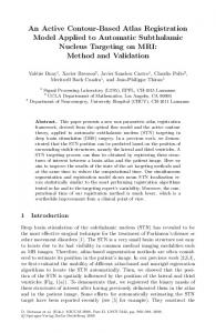
Local Sampling Grid Contour
Control Node
Figure 1.
Closed contour with control nodes and sampling grid
The window controls the sample size at each node (using a windows sized square discrete grid over which a node could move (see Figure 1); giving it a value of 0 will result in the contour failing to move, irrespective of any energy function parameters, as no alternative points for any node will be considered. A too large value will result in the contour making dramatic and erratic shapes in its morphology. Two other important parameters were defined as Minus and Maxus; these two parameters controlled the minimum and maximum allowed (straight line) distance between nodes; any drawn initial contour and any contour resulting from a call to the active control model would be redefined in terms of these two distances. The adopted active contour model algorithm would provide reasonable contours to well-defined high contrast features, such as the internal ventricles in MR and CT images but would fail to provide acceptable candidates for less well defined objects such as the thalamus and other white and grey-matter structures to be found in the imaged brain. For this reason a number of experiments were run to find changes to the original algorithm that would produce more acceptable contours; these are detailed below.
7
5. Advances On The Basic Model There are a number of simple modifications that were tried in order to improve the efficacy of the snake for our application. These include changes in the curvature measures, changes to the gradient operators and the addition of an extra component to the image energy. We also allowed the use of attractor, repulsor and static nodes. These initial changes are grouped together under the different energy components and the functional aspects of the active contour model algorithm. In its final state, the snake used an energy function of the form: Enode =
Alpha*Va + Beta*Vb + Gamma1*Vg + Gamma2*Vx + CoRepulse*VR + CoAttract*VA
where
Alpha
the elasticity coefficient
Beta
the stiffness coefficient
Gamma1
the edge gradient image energy coefficient
Gamma2
the zero-crossing image coefficient
CoRepulse
the Repulsor coefficient
CoAttract
the Attractor coefficient
Va,Vb
the measured internal values at the node
Vg
the edge gradient image value at the node
Vx
the zero crossings image value at the node
VA
the measured attraction value at the node
VR
the measured repulsion value at the node
The meaning and use of these terms becomes clearer in the following subsections.
New Algorithm The final algorithm for the active contour model developed under the auspices of the SAMMIE project works as follows:1. Initialisation. i)
Choose source image
ii)
Draw seed contour in approximate shape and location
iii)
Ensure control nodes are within minimum and maximum distance thresholds a) Remove node too close to neighbour b) Add node when neighbours too far apart
iiii)
Set up parameters
2. Call minimisation routine i)
Perform gradient operator on source image
ii)
Perform zero-crossing or canny approximation
iii)
Perform basic node checking
iiii)
Start iteration
v)
Call Global Shift
vi)
Call variation on Williams-Shah algorithm
vii)
Perform node checking if flagged
viii)
Continue iteration until
8
a) no change b) iteration parameter exceeded 3. Global Shift i)
Find max-min values for curvature, gradient, distance etc
ii)
Move all nodes to first offset on m*m global shift grid
iii)
Store position if lower energy
iv)
Repeat for all positions on global shift grid
v)
If lower energy snake found, move snake to that position.
4. Variation on Williams-Shah algorithm i)
Find max-min values for curvature, gradient, distance etc
ii)
Start at first node on snake
iii)
Calculate energy at this node
iiii)
Calculate energy if node were to move to first point on profile.
v)
Node migrates to new snake if energy lower at this point
vi)
Continue for all possible points in profile
vii)
Continue for all nodes
viii) Return new snake (may be exactly same as given snake) We can now turn the various components of this changed algorithm.
Sampling Space One change made to the active contour model, was the adoption of a profile based sampling space for the consideration of alternative coordinates for node placement, rather than a n*n discrete grid. Our early experiments with the original sampling method showed that ill-formed snakes were being produced too easily, so we constrained the search space.
Tangent To Node Contour
Control Node
Figure 2
Profile Based Sampling Space
The New Sampling Space
The tangent at a node is easily computed, so is the perpendicular to the tangent. The perpendicular to the tangent provides the basis for the profile space-sampling model adopted. Here the windows parameter rather than govern the size of a rectangular grid, is used to establish the point length of the profile; we actually use the original node coordinate plus a (windows length) profile out, and (windows length) in from that point. At each point of the profile, we consider a windows length tangent, with the central pixel on the normal profile (see figure 2). This actually gives us a sampling space of 2*windows+1 by windows, but unlike the original scheme 9
orientated about the tangent (and its normal) at the control node. This gave a definite improvement in the snake, at a slight computational cost. We also tried under sampling this space, to reduce the number of possible alternative positions for a node and so improve computational efficiency, but this gave poorer results.
Internal Energy A few changes to the method of calculating the two components to the internal energy were tried; this typically involved increasing the neighbourhood for the calculation of the internal energy components. These changes gave no observed improvement for the extra computational cost, so they were dropped.
Image Energy The image energy of the snake at any given node was changed so that it combines the output of two image processing techniques, and tends to shift nodes towards steep gradients in the image. One of these image processing techniques is a difference of Gaussian operator which produces a black image containing white edges (zero crossings). The other operator is a different form of edge operator which produces an edge gradient image. The zero crossings edge image (based on the Marr-Hildreth edge operator [25]) has the effect of pulling nodes towards zero crossings and away from non-zero crossings. The relevant coefficient, Gamma2, (taking a nominal value of 0.25) plays a similar role to Gamma1 in that controls the extent of this movement. Setting Gamma2 to 0 turns off the effect of zero crossings all together. The zero crossings operator is nominally given a lower Gaussian value, and the upper Gaussian value can be taken as 1.8 times the value of the lower Gaussian. As the zero crossing image is a binary image (where a point is either On or Off) , there is not the range of normalised values associated with this image as there is with the gradient image. If we were to simply use an integer (Boolean) value for a zero crossing image point, it is possible to produce a fluctuating erratic contour model. We have therefore designated two non-integer values for the two states; edge_off_weight (taking a nominal value of -0.10) for non-zero crossing points; and edge_on_weight (taking a nominal value of 0.15) for zero crossing points. It has been found that the Canny edge operator [26], with a SD of half the sum of the lower and upper Gaussian, acts as a good approximation to the zero crossing operator in most images but with less computational expense. Four alternative processes are allowed to produce the edge gradient map: the Mero-Vassey [27]; the Sobel edge detector [28]; a bidirectional morphological edge operator [29]; and the Canny edge operator [26]. The user is given control over which operator to use, with the Sobel as the default. Experiments show that the Sobel always out performed the Mero-Vassey, while the extra computational cost of the morphological operator was rewarded with better gradient information in gray-matter areas. For some areas in some images (notably greymatter areas in CT images), none of the operators provided reliable information, and that it normally paid to reduce the gradient coefficient (Gamma1). Improvements in computational efficiency were found by using a region of interest (ROI) for both image energy operators. The ROI is specified automatically to encompass the contour plus a border large enough to allow a considerable movement in the snake (during a global shift - see below) and in any change in morphology due to node migration. While we shall come to the fifth edge operator (or more correctly, the maximum likelihood edge detector MLD) at the end of this section (and in the section on future work); the testbed used for the development of the active contour model (and indeed the final Advanced Segmentation Module available in the Radiology Department at the Queen Elizabeth Hospital) does allow the use of this operator. When this is selected, no gradient image is used for local node migration as the MLD is one dimensional operator, but the Canny gradient image is used in the global shift algorithm (see below).
Constraint Energy The external constraint forces affecting the active contour model are attractor and repulsor forces from points in the image specified through user interaction. Attractor points are used to pull the contour towards a specific area, while repulsor points are used to ensure that the contour does not easily move towards a specific area. These two types of external force are not necessary for many features, and the active contour model will run without them; the provision of a means for specifying them allows a degree of flexibility in the use of the active contour model for finding accurate contours in noisy or busy image areas.
10
Repulsor points are used to stop the contour moving towards the areas where are placed; typically image areas of great contrast that are dragging the contour away from its desired shape. Repulsor points affect the movement of nodes in inverse ratio to the (normalised) distance between contour nodes and each repulsor point. A coefficient (Corepulse) controls the severity of this effect. As this coefficient is increased (from its nominal value of 0.15) the repulse energy is increased; conversely reducing this coefficient to 0 completely negates the effect of all the repulsor points. There is no limit to the number of repulsor points that can be used. We have found that when attempting to find highly convoluted brain structures (such as the sulci); setting up a central axis of repulsor points in the seed contour (with a low CoRepulse coefficient of less than 0.25) can be beneficial and tends to stop narrow contours crossing themselves. This will be discussed further in the section on future work. Attractor points are used to coerce the contour into moving towards the areas where are placed; typically image areas of poor contrast that are failing to drag the contour into its desired shape. Attractor points affect the movement of nodes in inverse ratio to the (normalised) distance between contour nodes and each attractor point. A coefficient (Coattract) controls the severity of this effect. As this coefficient is increased (from its nominal value of 0.15) the attraction energy is increased; conversely reducing this coefficient to 0 completely negates the effect of all the attractor points. There is no limit to the number of attractor points that can be used.
Dipoles and maximum likelihood detectors Dipoles are one dimensional edge detectors devised at the Wolfson Image Analysis Unit in Manchester [30]. They work by moving a window along a profile (an arbitrarily orientated line with a sampling width). Image informatics relating to the contents of the window give rise to informatics about the likelihood of an edge at that point along the profile. Maximum likelihood detectors are a development of this idea [31], but require no moveable sampling window. Instead, a moving divisor travels along the profile, and statistically based information about the likelihood of an edge at the divisors current position are amassed.
0
i
N-1
Figure 3 : A N Sized Dipole Placed On An Image Section Figure 3 shows a N sized MLD profile placed over a section of image. The size of the operator (here N = 5) is superimposed over an arbitrarily orientated profile of width W and length D. Typically the profile is orientated according to some higher order constraints; in the snake we use the perpendicular to a tangent at a contour controlling node. We arrange that W takes an odd integer value, while D is related to the local sample space parameter (actually D = 4*local). While we can specify the number of sampling spaces in the MLD (N), we have to ensure that the sampling space is great enough to allow meaningful statistics to be gathered (the standard deviation of the image pixel values in each sampling space). If this value is not great enough (we use a minimum value of 10 pixels per MLD sampling space, although there is room for experiment here), W is increased (in steps of 2 to remain odd). The MLD then produces maximum likelihood statistics for each sampling space. This it does by evaluating the standard deviation for the MLD as a whole; and the sds for each windows either side of the ith sampling space, from which the maximum likelihood can be calculated as follows:Maximum Likelihood, wi =
SDprofile N/2
/ [ SDAi/2 * SDA(N-i-1)/2 ]
This means that no statistics are gathered for the zero and (N-1) positions as there exists no window on one side for these positions. The MLD operator (when used in the snake works as follows):1.
Call MLD operator with current node CN.
i)
initialise W as 3/4 distance from previous to next node, and increase by 1 if even value.
ii)
initialise minimum sampling space MinS to 10.
iii)
set N to be twice local parameter plus 1. 11
iv)
set profile size D to 8 times local parameter.
v)
set window sample space WSS to be D over N.
vi)
make MLD structure
vii)
run MLD and clean up unwanted information.
viii)
return MLD structure to calling routine
2.
Make MLD structure
i)
while W*WSS less than MinS increment W by 2.
ii)
set up memory areas for information gathering
iii)
sample image over real coordinate profile to produce a local sampled image of size W by D.
iv)
return MLD structure
3. i)
Run MLD operator for each MLD sampling window, calculate:a)
number of pixel points
b)
sum of pixel values
c)
sum of the squares of the pixel values
ii)
using all these statistics calculate sd for MLD as a whole.
ii)
step through MLD sampling space (i