The characteristic function for Jacobi matrices with applications

The characteristic function for Jacobi matrices with applications

arXiv:1201.1743v1 [math.SP] 9 Jan 2012

F. Štampach, P. Šťovíček Department of Mathematics, Faculty of Nuclear Science, Czech Technical University in Prague, Trojanova13, 12000 Praha, Czech Republic

Abstract We introduce a class of Jacobi operators with discrete spectra which is characterized by a simple convergence condition. With any operator J from this class we associate a characteristic function as an analytic function on a suitable domain, and show that its zero set actually coincides with the set of eigenvalues of J in that domain. Further we derive sufficient conditions under which the spectrum of J is approximated by spectra of truncated finite-dimensional Jacobi matrices. As an application we construct several examples of Jacobi matrices for which the characteristic function can be expressed in terms of special functions. In more detail we study the example where the diagonal sequence of J is linear while the neighboring parallels to the diagonal are constant.

Keywords: infinite Jacobi matrix, spectral problem, characteristic function

1

Introduction

In this paper we introduce and study a class of infinite symmetric but in general complex Jacobi matrices J characterized by a simple convergence condition. This class is also distinguished by the discrete character of spectra of the corresponding Jacobi operators. Doing so we extend and generalize an approach to Jacobi matrices which was originally initiated, under much more restricted circumstances, in [20]. We refer to [16] for a rather general analysis of how the character of spectrum of a Jacobi operator may depend on the asymptotic behavior of weights. For a given Jacobi matrix J , one constructs a characteristic function FJ (z) as an analytic function on the domain Cλ0 obtained by excluding from the complex plane the closure of the range of the diagonal sequence λ of J . Under some comparatively simple additional assumptions, like requiring the real part of λ to be semibounded or J to be real, one can show that J determines a unique closed Jacobi operator J on ℓ2 (N). Moreover, the spectrum of J in the domain Cλ0 is discrete and coincides with 1

the zero set of FJ (z). When establishing this relationship one may also treat the poles of FJ (z) which occur at the points from the range of the sequence λ not belonging to the set of accumulation points, however. In addition, as an important step of the proof, one makes use of an explicit formula for the Green function associated with J. Apart of the localization of the spectrum we address too the question of approximation of the spectrum by spectra of truncated finite-dimensional Jacobi matrices. For bounded Hermitian Jacobi operators the problem has been studied, for example in [11, 3, 13]. We are aware of just a few papers, however, bringing some results in this respect also about unbounded Jacobi operators [14, 12, 18]. Our approach based on employing the characteristic function makes it possible to derive sufficient conditions under which such an approximation can be verified. This result partially reproduces and overlaps with some theorems from [12]. The characteristic function as well as numerous formulas throughout the paper are expressed in terms of a function, called F, defined on a subset of the space of complex sequences. In the introductory part we recall from [20] the definition of F and its basic properties which are then completed by various additional facts. On the other hand, we conclude the paper with some applications of the derived results. We present several examples of Jacobi matrices for which the characteristic function can be expressed in terms of special functions (the Bessel functions or the basic hypergeometric series). A particular attention is paid to the example where the diagonal sequence λ is linear while the neighboring parallels to the diagonal are constant. In this case the characteristic equation in the variable z reads J−z (2w) = 0, with w being a parameter, and our main concern is how the spectrum of the Jacobi operator depends on w.

The function F

2 2.1

Definition and basic properties

Let us recall from [20] some basic definitions and properties concerning a function F defined on a subset of the linear space formed by all complex sequences x = {xk }∞ k=1 . Moreover, we complete this brief overview by a few additional facts. Definition 1. Define F : D → C, F(x) = 1 +

∞ X

m=1

(−1)

m

∞ X

∞ X

k1 =1 k2 =k1 +2

where D=

(

∞ X

...

xk1 xk1 +1 xk2 xk2 +1 . . . xkm xkm +1 , (1)

km =km−1 +2

{xk }∞ k=1 ⊂ C;

∞ X k=1

)

|xk xk+1 | < ∞ .

For a finite number of complex variables we identify F(x1 , x2 , . . . , xn ) with F(x) where x = (x1 , x2 , . . . , xn , 0, 0, 0, . . . ). By convention, we also put F(∅) = 1 where ∅ is the empty sequence.

2

Let us remark that the value of F on a finite complex sequence can be expressed as the determinant of a finite Jacobi matrix. Using some basic linear algebra it is easy to show that, for n ∈ N and {xj }nj=1 ⊂ C, one has (2)

F(x1 , x2 , . . . , xn ) = det Xn where

 1 x1 x2 1 x2    .. .. ..   . . .   Xn =  . . . .   .. .. ..    xn−1 1 xn−1  xn 1 

Note that the domain D is not a linear space. One has, however, ℓ2 (N) ⊂ D. In fact, the absolute value of the mth summand on the RHS of (1) is majorized by the expression !m ∞ X 1 X |xk1 xk1 +1 xk2 xk2 +1 . . . xkm xkm +1 | ≤ |xj xj+1 | . m! j=1 m k∈N k1 n0 one has q q 1 1 (1) (1) (2) (2) |wn | ≤ |ζn ||ζn+1| , |wn | ≤ |ζn ||ζn+1| . 2 2

Using (3), after some straightforward manipulations one gets the estimate ! n ∞ 0 w2 Y 2 2 X w w k−1 (2) (1) k(1) + (2) k(2) wn fn(1) fn+1 ≤ 2−2(n−n0 ) exp (1) (2) ζ ζ k=1 ζk ζk+1 k k+1 k=1 ζk ζk

This implies (25).

|wn | × |ζn(1) ζ (2) |1/2 . 0 n0 (1) (2) 1/2 ζn ζn+1

In the literature on Jacobi matrices one encounters a construction of an infinite matrix associated with the bilateral difference equation (20) [21, § 1.1], [10, Theorem 1.2]. Let us define the matrix J with entries J(m, n), m, n ∈ Z, so that for every fixed m, the sequence un = J(m, n), n ∈ Z, solves (20) with the initial conditions J(m, m) = 0, J(m, m + 1) = 1/wm. Using (6) one verifies that, for m < n, !   n−1 2 2 2 Y ζj γm+1 γm+2 γn−1 1 J(m, n) = F . , ,..., wm j=m+1 wj ζm+1 ζm+2 ζn−1 Moreover, it is quite obvious that, for all m, n ∈ Z, J(m, n) =

1 (um vn − vm un ) , W(u, v) 9

where {un }, {vn } is any couple of independent solutions of (20). Hence the matrix J is antisymmetric. It also follows that, ∀m, n, k, ℓ ∈ Z, J(m, k)J(n, ℓ) − J(m, ℓ)J(n, k) = J(m, n)J(k, ℓ). Example 7. As an example let us again have a look at the particular case where wn = w, ζn = ν + n for all n ∈ Z and some w, ν ∈ C, w 6= 0, ν ∈ / Z. One finds, with the aid of (15), that the solutions (21) now read fn = Γ(ν + 1) w −ν Jν+n (2w), gn =

(−1)n π w ν J−ν−n (2w). sin(πν)Γ(ν + 1)

Hence the Wronskian equals πw (−Jν (2w)J−ν−1(2w) − Jν+1 (2w)J−ν (2w)) = F W(f, g) = sin(πν)



w ν +n

∞

n=−∞

 .

Recalling once more (15) we note that the RHS equals

lim F

N →∞



w ν −N +n

∞  n=1

= lim

N →∞

∞ X (−1)n n=0

n!

Γ(ν − N + 1) w 2n = 1. Γ(ν − N + n + 1)

Thus one gets the well known relation [1, Eq. 9.1.15] sin(πν) . (26) πw Concerning the matrix J, this particular choice brings us to the case discussed in [20, Proposition 22]. Then the Bessel functions Yn+ν (2w) and Jn+ν (2w), depending on the index n ∈ Z, represent other two linearly independent solutions of (20). Since [1, Eq. 9.1.16] 2 Jν+1 (z)Yν (z) − Jν (z)Yν+1 (z) = πz one finds that Jν+1 (2w)J−ν (2w) + Jν (2w)J−ν−1(2w) = −

J(m, n) = π (Ym+ν (2w)Jn+ν (2w) − Jm+ν (2w)Yn+ν (2w)) . Moreover, for σ = m + µ and k = n − m > 0 one has Γ(σ + k) Jσ+k (2w)Yσ (2w) − Jσ (2w)Yσ+k (2w) = F πw k Γ(σ + 1) (1)

(2)



w σ+j

k−1!

.

j=1

Finally, putting ζn = µ + n, ζn = ν + n and wn = w, ∀n ∈ N, in equation (22), one verifies that (24) holds true and reveals this way once more the identity (18).

10

3

A class of Jacobi operators with point spectra

3.1

The characteristic function

Being inspired by Proposition 4 and notably by equation (13), we introduce the (renormalized) characteristic function associated with a Jacobi matrix J as ∞   γn2 . (27) FJ (z) := F λn − z n=1 It is treated as a complex function of a complex variable z and is well defined provided the sequence in the argument of F belongs to the domain D. Let us show that this is guaranteed under the assumption that there exists z0 ∈ C such that ∞ X wn2 (28) (λn − z0 )(λn+1 − z0 ) < ∞. n=1 For λ = {λn }∞ n=1 let us denote

Cλ0 := C \ {λn ; n ∈ N}. Clearly, {λn ; n ∈ N} = {λn ; n ∈ N} ∪ der(λ)

where der(λ) stands for the set of all finite accumulation points of the sequence λ (i.e., der(λ) is equal to the set of limit points of all possible convergent subsequences of λ). Lemma 8. Let condition (28) be fulfilled for at least one z0 ∈ Cλ0 . Then the series ∞ X n=1

wn2 (λn − z)(λn+1 − z)

converges absolutely and locally uniformly in z on Cλ0 . Moreover,  n  γk2 λ ∀z ∈ C0 , lim F = FJ (z), n→∞ λk − z k=1

(29)

(30)

and the convergence is locally uniform on Cλ0 . Consequently, FJ (z) is a well defined analytic function on Cλ0 . Proof. Let K ⊂ Cλ0 be a compact subset. Then the ratio |z − z0 | |λn − z0 | ≤1+ |λn − z| |λn − z| admits an upper bound, uniform in z ∈ K and n ∈ N. The uniform convergence on K of the series (29) thus becomes obvious. 11

The limit (30) follows from Lemma 2. Moreover, using (30) and also (6), (3) one has   n  l ! l+1 !  ∞ 2 2 2 X γ γ γ k k k F − FJ (z) ≤ −F F λk − z k=1 λk − z k=1 λk − z k=1 l=n ! ∞ ∞ 2 2 X X w w k l exp ≤ (λk − z)(λk+1 − z) . (λl − z)(λl+1 − z) k=1 l=n

From this estimate and the locally uniform convergence of the series (29) one deduces the locally uniform convergence of the sequence of functions (30). By a closer inspection one finds that, under the assumptions of Lemma 8, the function FJ (z) is meromorphic on C \ der(λ) with poles at the points z = λn for some n ∈ N (not belonging to der(λ), however). For any such z, the order of the pole is less than or equal to r(z) where ∞ X δz,λk r(z) := k=1

is the number of members of the sequence λ coinciding with z (hence r(z) = 0 for z ∈ Cλ0 ). To see this, suppose that r(z) ≥ 1 and let M be the maximal index such that λM = z. Using (4) one derives that, for u ∈ Cλ0 ,  M !  ∞  2 γn γn2 FJ (u) = F F λn − u n=1 λn − u n=M +1 !  ∞    M −1 2 2 γM γM +1 γn2 γn2 . F +F λn − u n=1 (u − z)(λM +1 − u) λn − u n=M +2 The RHS clearly has a pole at the point u = z of order at most r(z).

3.2

The Jacobi operator J

Our goal is to investigate spectral properties of a closed operator J on ℓ2 (N) whose matrix in the standard basis coincides with J . Provided the Jacobi matrix does not determine a bounded operator, however, there need not be a unique way how to introduce J. But among all admissible operators one may distinguish two particular cases which may respectively be regarded, in a natural way, as the minimal and the maximal operator with the required properties; see, for instance, [4]. Definition 9. The operator Jmax is defined so that Dom(Jmax ) = {y ∈ ℓ2 (N); J y ∈ ℓ2 (N)},

and one sets Jmax y = J y, ∀y ∈ Dom Jmax . Here and in what follows J y is understood as the formal matrix product while treating y as a column vector. To define the ˙ is the linear hull of operator Jmin one first introduces the operator J˙ so that Dom(J) ˙ = J y for all y ∈ Dom(J). ˙ J˙ is known to be closable the standard basis, and again Jy ˙ [4], and Jmin is defined as the closure of J. 12

One has the following relations between the operators Jmin , Jmax and their adjoint operators [4, Lemma 2.1]. Let J H designates the Jacobi matrix obtained from J ∗ H ∗ H by taking the complex conjugate of each entry. Then Jmin = Jmax , Jmax = Jmin . In particular, the maximal operator Jmax is a closed extension of Jmin . It is even true that any closed operator J whose domain contains the standard basis and whose matrix in this basis equals J fulfills Jmin ⊂ J ⊂ Jmax . Moreover, if J is Hermitian, i.e. ∗ J = J H (which means nothing but J is real), then Jmin = Jmax ⊃ Jmin . Hence Jmin is symmetric with the deficiency indices either (0, 0) or (1, 1). We are primarily interested in the situation where Jmin = Jmax since then there exists a unique closed operator J defined by the Jacobi matrix J , and it turns out that the spectrum of J is determined in a well defined sense by the characteristic function FJ (z). If this happens J is sometimes called proper [4]. Let us recall more details on this property. We remind the reader that the orthogonal polynomials of the first kind, pn (z), are defined by the recurrence wn−1 pn−1 (z) + λn pn (z) + wn pn+1 (z) = z pn (z),

n = 1, 2, 3, . . . ,

with the initial conditions p0 (z) = 1, p1 (z) = (z −λ1 )/w1. The orthogonal polynomials of the second kind, qn (z), obey the same recurrence but the initial conditions are q0 (z) = 0, q1 (z) = 1/w1; see [2, 5]. It is not difficult to verify that these polynomials are expressible in terms of the function F as follows: !  n  n Y z − λk γl2 pn (z) = F , n = 0, 1, 2 . . . , wk λl − z l=1 k=1

and

1 qn (z) = w1

n Y z − λk wk k=2

!  n  γl2 F , λl − z l=2

n = 1, 2, 3 . . . .

The complex Jacobi matrix J is called determinate if at least one of the sequences ∞ 2 p(0) = {pn (0)}∞ n=0 or q(0) = {qn (0)}n=0 is not an element of ℓ (Z+ ). For real Jacobi matrices there exits a parallel terminology. Instead of determinate one calls J limit point at +∞, and instead of indeterminate one calls J limit circle at +∞, see [21, p. 48]. According to [22, Theorem 22.1], J is indeterminate if both p(z) and q(z) are elements of ℓ2 for at least one z ∈ C, and in this case they are elements of ℓ2 for all z ∈ C. For a real Jacobi matrix J one can prove that it is proper if and only if it is determinate (or, in another terminology, limit point), see [2, pp. 138-141] or [21, Lemma 2.16]. For complex Jacobi matrices one can also specify assumptions under which Jmin = Jmax . In what follows, ρ(A) designates the resolvent set of a closed operator A. Concerning the essential spectrum, one observes that specess (Jmin ) = specess (Jmax ) [4, Eq. 2.10]. Hence if ρ(Jmax ) 6= ∅ then specess (Jmin) 6= C. Moreover, in that case J is determinate [4, Theorem 2.11 (a)] and proper [4, Theorem 2.6 (a)]. This way one extracts from [4] the following result. Theorem 10. If ρ(Jmax ) 6= ∅ then Jmin = Jmax . 13

3.3

The spectrum and the zero set of the characteristic function

Let us define n o Z(J ) := z ∈ C \ der(λ); lim (u − z)r(z) FJ (u) = 0 . u→z

(31)

Of course, Z(J ) ∩ Cλ0 is nothing but the set of zeros of FJ (z). Further, for k ∈ Z+ and z ∈ C \ der(λ) we put !  ∞  k Y γl2 w l−1 r(z) F , (32) ξk (z) := lim (u − z) u→z u − λ λ l l − u l=k+1 l=1

where one sets w0 = 1. One observes that for k ≥ M, where M = Mz is either the maximal index, if any, such that z = λM , or M = 0 otherwise, !−1  ∞  k k Y Y γl2 (z − λl ) F ξk (z) = wl−1 . (33) λl − z l=k+1 l=1 l=1 λl 6=z

Proposition 11. Let condition (28) be fulfilled for at least one z0 ∈ Cλ0 . If ξ0 (z) ≡ lim (u − z)r(z) FJ (u) = 0 u→z

for some z ∈ C \ der(λ), then z is an eigenvalue of Jmax and ξ(z) := (ξ1 (z), ξ2 (z), ξ3 (z), . . .) is the corresponding eigenvector. Proof. Using (5) one verifies that if ξ0 (z) = 0 then the column vector ξ(z) solves the matrix equation J ξ(z) = zξ(z). To complete the proof one has to show that ξ(z) does not vanish and belongs to ℓ2 (N). First, we claim that ξ1 (z) 6= 0. Suppose, on the contrary, that ξ1 (z) = 0. Then the formal eigenvalue equation (which is a second order recurrence) implies ξ(z) = 0. From (33) it follows that ∞   γl2 =0 F λl − z l=k+1

for all k ≥ M = Mz . This equality is in contradiction with (7), however. Second, suppose z ∈ / der(λ) is fixed. By Lemma 8, there exists N ∈ N, N > M, such that |wn2 | ≤ |λn − z||λn+1 − z|/2, ∀n ≥ N. Let us denote

C=

N Y l=1

|wl−1|

2

N Y

l=1 λl 6=z

14

|z − λl |−2 .

Using also (3) one can estimate ∞ X

k=N

2

|ξk (z)| =

∞ Y k X

k=N l=1

|wl−1 |

2

k Y

l=1 λl 6=z

|z − λl |

 ∞ γl2 F λl − z

−2

l=k+1

 2

! ∞  k  ∞ 2 X X Y z − λl−1 1 w k ≤ C exp 2 z − λl . (λk − z)(λk+1 − z) 2 k=N l=N +1 k=N +1

Since |λk − z| ≥ τ for all k > M and some τ > 0, the RHS is finite.

Further we wish to prove a statement converse to Proposition 11. Our approach is based on a formula for the Green function generalizing a similar result known for the finite-dimensional case; see (14). Proposition 12. Let condition (28) be fulfilled for at least one z0 ∈ Cλ0 . If z ∈ C\ der(λ) does not belong to the zero set Z(J ) then z ∈ ρ(Jmax ) and the Green function for the spectral parameter z, G(z; i, j) := hei , (Jmax − z)−1 ej i, i, j ∈ N, (a matrix in the standard basis) is given by the formula   max(i,j) Y wl  1  (34) G(z; i, j) = − wmax(i,j) z − λl l=min(i,j) !   min(i,j)−1 !  ∞ ∞ −1 γl2 γl2 γl2 ×F . F F λl − z l=1 λl − z l=max(i,j)+1 λl − z l=1 In particular, for the Weyl m-function one has 1 F m(z) := G(z; 1, 1) = λ1 − z



γl2 λl − z

∞   ∞ −1 γl2 . F λl − z l=1 l=2

(35)

If, in addition, |λn | → ∞ as n → ∞ then der(λ) = ∅ and for every z ∈ C\Z(J ), the resolvent (Jmax − z)−1 is compact. Proof. Denote by R(z)i,j the RHS of (34). Thus R(z) is an infinite matrix provided its entries R(z)i,j , i, j ∈ N, make good sense. Suppose that a complex number z does not belong to Z(J) ∪ der(λ). By Lemma 8, in that case the RHS of (34) is well defined. By inspection of the expression one finds that this is so even if z happens to coincide with a member λk of the sequence λ not belonging to der(λ), i.e. the seeming singularity at z = λk is removable. For the sake of simplicity we assume in the remainder of the proof, however, that z does not belong to the range of the sequence λ. The only purpose of this assumption is just to simplify the discussion and to avoid more complex expressions but otherwise it is not essential for the result. 15

First let us show that there exists a constant C, possibly depending on z but independent of the indices i, j, such that |R(z)i,j | ≤ C 2−|i−j|, ∀i, j ∈ N.

(36)

To this end, denote τ = inf{|z − λn |; n ∈ N} > 0.

Assuming (28), one can choose n0 ∈ N so that, for all n ≥ n0 , |wn |2 ≤ |λn − z| |λn+1 − z|/4.

(37)

Let us assume, for the sake of definiteness, that i ≤ j. Again by (28) and (3),  i−1 !  ∞ !  ∞ −1 γl2 γl2 γl2 F F F ≤ C1 , λl − z l=1 λl − z l=j+1 λl − z l=1 for all i, j. It remains to estimate the expression j−1 1 Y wl . |λj − z| l=i λl − z

(38)

We distinguish three cases. For the finite set of couples i, j, i ≤ j ≤ n0 , (38) is bounded from above by a constant C2 . Using (37), if i ≤ n0 ≤ j then (38) is majorized by j−1 λ − z Y w n l C2 0 ≤ C2 τ −1/2 |λn0 − z|1/2 2−j+n0 . λj − z λl − z l=n0

Similarly, if n0 ≤ i ≤ j then (38) is majorized by τ −1 2−j+i . From these partial upper bounds the estimate (36) readily follows. From (36) one deduces that the matrix R(z) represents a bounded operator on 2 ℓ (N). In fact, one can write R(z) as a countable sum, X R(z) = R(z; s), (39) s∈Z

where the matrix elements of the summands are R(z; s)i,j = R(z)i,j if i − j = s and R(z; s)i,j = 0 otherwise. Thus R(z; s) has nonvanishing elements on only one parallel to the diagonal and kR(z; s)k = sup{|R(z)i,j |; i − j = s} ≤ C 2−|s| . Hence the series (39) converges in the operator norm. With some abuse of notation, we shall denote the corresponding bounded operator again by the symbol R(z). Further one observes that, on the level of formal matrix products, (J − z)R(z) = R(z)(J − z) = I. 16

The both equalities are in fact equivalent to the countable system of equations (with w0 = 0) wk−1 G(z; i, k − 1) + (λk − z)G(z; i, k) + wk G(z; i, k + 1) = δi,k , i, k ∈ N. This can be verified, in a straightforward manner, with the aid of the rule (4) or some of its particular cases (5) and (6). By inspection of the domains one then readily shows that the operators Jmax − z and R(z) are mutually inverse and so z ∈ ρ(Jmax ). Finally, suppose that |λn | → ∞ as n → ∞, and z ∈ C \ Z(J ). It turns out that then the above estimates may be somewhat refined. In particular, (38) is majorized by |λi − z|−1/2 |λj − z|−1/2 2−j+i for n0 ≤ i, j. But this implies that R(z; s)i,j → 0 as i, j → ∞, with i − j = s being constant. It follows that the operators R(z; s) are compact. Since the series (39) converges in the operator norm, R(z) is compact as well.

Corollary 13. If condition (28) is fulfilled for at least one z0 ∈ Cλ0 then spec(Jmax ) \ der(λ) = specp (Jmax ) \ der(λ) = Z(J ). Proof. Propositions 11 and 12 respectively imply the inclusions Z(J ) ⊂ specp (Jmax ) \ der(λ), spec(Jmax ) \ der(λ) ⊂ Z(J ). This shows the equality. Theorem 14. Suppose that the convergence condition (28) is fulfilled for at least one z0 ∈ Cλ0 and the function FJ (z) does not vanish identically on Cλ0 . Then Jmin = Jmax =: J and spec(J) \ der(λ) = specp (J) \ der(λ) = Z(J ). (40) Suppose, in addition, that the set C\ der(λ) is connected. Then spec(J)\der(λ) consists of simple eigenvalues which have no accumulation points in C \ der(λ). Proof. By the assumptions, C \ (der(λ) ∪ Z(J )) 6= ∅. From Proposition 12 one infers that ρ(Jmax ) 6= ∅. According to Theorem 10, one has Jmin = Jmax . Then (40) becomes a particular case of Corollary 13. Let us assume that C\ der(λ) is connected. Then the set Cλ0 is clearly connected as well. Suppose on contrary that the point spectrum of J has an accumulation point in C \ der(λ). Then, by equality (40), the set of zeros of the analytic function FJ (z) has an accumulation point in C \ der(λ). This accumulation point may happen to be a member λn of the sequence λ, but then one knows that FJ (z) has a pole of finite order at λn . In any case, taking into account that Cλ0 is connected one comes to the conclusion that FJ (z) = 0 everywhere on Cλ0 , a contradiction.

17

Remark 15. Theorem 14 is derived under two assumptions: (i) The convergence condition (28) is fulfilled for at least one z0 ∈ Cλ0 . (ii) The function FJ (z) does not vanish identically on Cλ0 . But let us point out that assumption (ii) is automatically fulfilled if (i) is true and the range of the sequence λ is contained in a halfplane. This happens, for example, if the sequence λ is real or the sequence {Re λn }∞ n=1 is semibounded. In fact, let us for definiteness consider the latter case and suppose that Re λn ≥ c, ∀n ∈ N. Then (−∞, c) ⊂ Cλ0 and 1/|λn − z| tends to 0 monotonically for all n as z → −∞. Similarly as in (3) one derives the estimate ! ∞ 2 X wn |FJ (z) − 1| ≤ exp (λn − z)(λn+1 − z) − 1. n=1 It follows that limz→−∞ FJ (z) = 1. Notice that in the real case, the function FJ (z) can identically vanish neither on the upper nor on the lower halfplane.

Corollary 16. Let J be real and suppose that (28) is fulfilled for at least one z0 ∈ Cλ0 . Then Jmin = Jmax = J is self-adjoint and spec(J) \ der(λ) = Z(J ) consists of simple real eigenvalues which have no accumulation points in R \ der(λ). Proof. Some assumptions in Theorem 14 become superfluous if J is real. As observed in Remark 15, assuming the convergence condition the function FJ (z) cannot vanish identically on Cλ0 . The operator J is self-adjoint and may have only real eigenvalues. The set C \ der(λ) may happen to be disconnected only if the range of the sequence λ is dense in R, i.e. der(λ) = R. But even then the conclusion of the theorem remains trivially true. Let us complete this analysis by a formula for the norms of the eigenvectors described in Proposition 11. In order to simplify the discussion we restrict ourselves to the domain Cλ0 . Then instead of (32) one may write !  ∞  k Y γl2 wl−1 F , z ∈ Cλ0 , k ∈ Z+ . (41) ξk (z) = z − λ λ − z l l l=k+1 l=1 This is in fact nothing but the solution fn from (21) restricted to nonnegative indices. Proposition 17. If z ∈ Cλ0 satisfies (28) then the functions ξk (z), k ∈ Z+ , defined in (41) fulfill ∞ X ξk (z)2 = ξ0′ (z)ξ1 (z) − ξ0 (z)ξ1′ (z). (42) k=1

Particularly, if in addition J is real and z ∈ R ∩ Cλ0 is an eigenvalue of J then ξ(z) = (ξk (z))∞ k=1 is a corresponding eigenvector and kξ(z)k2 = ξ0′ (z)ξ1 (z). 18

(43)

(1)

(2)

Proof. Put ζj = z − λj , ζj = y − λj , j ∈ N, in equation (23), where z, y ∈ Cλ0 . Then (1) (2) Proposition 6 is applicable to fj = ξj (z), fj = ξj (y), j ∈ Z+ . Hence (w0 = 1) (z − y)

∞ X k=0

ξk (z)ξk (y) = ξ1 (z)ξ0 (y) − ξ0 (z)ξ1 (y).

Now the limit y → z can be treated in a routine way.

Corollary 18. Suppose J is real and let condition (28) be fulfilled for at least one z0 ∈ Cλ0 . Then the function FJ (z) has only simple real zeros on Cλ0 .

Proof. Suppose z ∈ Cλ0 is a zero of FJ (z), i.e. FJ (z) ≡ ξ0 (z) = 0. Then z is a real eigenvalue of J where J = Jmax = Jmin is self-adjoint, as we know from Corollary 16. Moreover, by Proposition 11, ξ(z) 6= 0 is a corresponding real eigenvector. Hence from (43) one infers that necessarily ξ0′ (z) 6= 0.

3.4

Approximation of the spectrum by spectra of truncated matrices

Let us first introduce some additional notation which will be needed in the current subsection. W and L stand for the diagonal matrix operators whose diagonals equal w and λ, respectively. U designates the unilateral shift and U ∗ its adjoint operator (Uen = en+1 for n = 1, 2, 3, . . . , with en being the vectors of the standard basis). For a Jacobi matrix J we introduce the set Λ(J ) := {µ ∈ C; lim dist(spec(Jn ), µ) = 0} n→∞

(44)

where Jn is defined in (10) but now with v = w. Thus µ ∈ Λ(J ) iff there exists a sequence of eigenvalues {µn } of Jn such that µn → µ as n → ∞. Remark 19. (i) Definition (44) is taken, for example, from [3]. Some authors prefer ˜ ) formed by all limit points of sequences {µk } of to work, however, with the set Λ(J eigenvalues from spec(Jnk ), with {nk } being any possible strictly increasing sequence ˜ ) and the inclusion is in general strict of indices [11, 12]. One clearly has Λ(J ) ⊂ Λ(J as demonstrated by a simple example in [11, Eq. (2)]. (ii) In the case where the sequences λ and w are real and positive, respectively, the relation between the spectrum of a Jacobi operator J and the set Λ(J ) has been intensively studied by several authors. Most results of this kind are restricted to the bounded case, however. The inclusion spec(J) ⊂ Λ(J ) is proved for bounded Jacobi matrices in [3, Theorem 2.3]. It cannot be replaced, in general, by the sign of equality as demonstrates an counterexample constructed in the Appendix in [3]. (iii) In [14, Theorem 5.1] it is shown that spec(JS ) ⊂ Λ(J ) where the operator JS := L + W U ∗ + UW

(an operator sum) is assumed to be self-adjoint. Some reasoning used below, notably that in Lemmas 21 and 22, is inspired by this article. We also remark that Theorem 23 below partially reproduces and overlaps with Theorems 2.1 and 2.10 from [12]. 19

Lemma 20. If condition (28) is fulfilled for at least one z0 ∈ Cλ0 then Λ(J ) \ der(λ) ⊂ Z(J ).

(45)

Proof. Let z ∈ Λ(J ) \ der(λ). Then, by definition, there exists a sequence {µn } such that µn ∈ spec(Jn ) and µn → z as n → ∞. Considering sufficiently large indices n one may assume that µn does not coincide with any member λk of the sequence λ, possibly except of z. Using (13) one gets, for all sufficiently large n,    n  n γl2  Y r(z) (µn − λk ) lim (u − z) F 0 = det(µn In − Jn ) =  . (46) u→µn λ l − u l=1 k=1 λk 6=z

Denote temporarily ˜n

F (u) = (u − z)

r(z)

F



γl2 λl − u

n  , u ∈ Cλ0 , n ∈ N ∪ {∞}. l=1

All functions F˜ n (u) have a removable singularity at u = z. Moreover, with some slight modification of Lemma 8 one can show that F˜ n (u) → F˜ ∞ (u) as n → ∞ uniformly on a neighborhood of the point z. Since all the involved functions are analytic on this domain, one knows that the corresponding derivatives converge uniformly as well. Equation (46) means that F˜ n (µn ) = 0 for all n sufficiently large. One concludes that lim (u − z)r(z) FJ (u) = F˜ ∞ (z) = lim F˜ n (µn ) = 0.

u→z

n→∞

Hence z ∈ Z(J ). Denote by Pn , n ∈ N, the orthogonal projection on ℓ2 (N) onto the linear hull of the first n vectors of the standard basis. Then the finite-dimensional operator Jn introduced in (10) can be identified with Pn JPn restricted to the subspace Ran Pn . Here J is any operator such that J˙ ⊂ J (see Definition 9). Lemma 21. Let J be any operator on ℓ2 (N) fulfilling J˙ ⊂ J. Then (in ℓ2 (N)) lim Pn JPn x = Jx, ∀x ∈ Dom(J) ∩ Dom(W U ∗ ).

n→∞

Proof. Let x ∈ Dom(J) ∩ Dom(W U ∗ ). Since (J − Pn JPn )x = (I − Pn )Jx + Pn J(I − Pn )x one has k(J −Pn JPn )xk2 = k(I −Pn )Jxk2 + |wn |2 |hx, en+1 i|2 = k(I −Pn )Jxk2 + |hW U ∗ x, en i|2 . The RHS clearly tends to zero as n → ∞. 20

Lemma 22. Suppose that J is real and let J be a self-adjoint extension of the symmetric operator Jmin . If Dom(J) ⊂ Dom(W U ∗ ) then spec(J) ⊂ Λ(J ). If, in addition, condition (28) is fulfilled for at least one z0 ∈ Cλ0 then Z(J ) = spec(J) \ der(λ) = specp (J) \ der(λ) = Λ(J ) \ der(λ).

(47)

Proof. First suppose that, on the contrary, µ ∈ spec(J) and µ ∈ / Λ(J ). Then there ∞ exist d > 0 and a subsequence {Jnk }k=1 such that dist(µ, spec Jnk ) ≥ d for all k. Let x be an arbitrary vector from Dom(J) ⊂ Dom(W U ∗ ). As is well known and easy to verify, if A is a self-adjoint operator such that 0 belongs to its resolvent set then kA−1 k ≤ 1/ dist(0, spec A). This implies that ∀f ∈ Dom A, kAf k ≥ dist(0, spec A)kf k. Applying this observation to the operators Jnk one gets k(µPnk − Pnk JPnk )xk ≥ dkPnk xk. Sending k → ∞ and referring to Lemma 21 one concludes that k(µ − J)xk ≥ dkxk, for every x ∈ Dom(J). By the Weyl criterion µ ∈ ρ(J), a contradiction. If, in addition, (28) is fulfilled for at least one z0 ∈ Cλ0 then we know from Corollary 16 that J is in fact unique and the first two equalities in (47) are true. So combination of Lemma 20 with the first part of the current lemma yields Z(J ) = spec(J) \ der(λ) ⊂ Λ(J ) \ der(λ) ⊂ Z(J ). This completes the proof. Theorem 23. Suppose that the Jacobi matrix J is real and let condition (28) be fulfilled for at least one z0 ∈ Cλ0 . If any of the following two conditions is satisfied: (i) limn→∞ wn = 0, (ii) limn→∞ |λn | = ∞ and lim sup n→∞

|wn | |wn | + lim sup < 1, |λn | n→∞ |λn+1 |

(48)

then Λ(J ) = spec(J),

(49)

where J is the unique self-adjoint operator whose matrix in the standard basis equals J. Proof. According to Corollary 16, J = Jmin = Jmax is the unique self-adjoint operator determined by J . (i) Let limn→∞ wn = 0. Then we claim that der(λ) = specess (J) ⊂ spec(J) ⊂ Λ(J ). 21

(50)

In fact, the Hermitian operator W U ∗ + UW is compact and J = L + (W U ∗ + UW )

(51)

(an operator sum, Dom J = Dom L). But the Weyl theorem tells us that J has the same essential spectrum as L, which is nothing but der(λ). The last inclusion in (50) follows from Lemma 22. Again by Lemma 22, spec(J) \ der(λ) = Λ(J ) \ der(λ), which jointly with (50) implies (49). (ii) Suppose that |λn | → ∞ and (48) is true. Then clearly der(λ) = ∅. We wish to verify the assumptions of Lemma 22. Since the sum of a self-adjoint operator with a bounded Hermitian operator does not change the domain one may suppose, without loss of generality, that |λn | ≥ 1, ∀n, and sup n

|wn | |wn | + sup ≤ α < 1, |λn | n |λn+1 |

where α is a constant. But this means that k(W U ∗ + UW )L−1 k ≤ kW U ∗ L−1 k + kW L−1 k ≤ α, and hence (W U ∗ + UW ) is L-bounded with a relative bound smaller than 1. By the Kato-Rellich theorem [17, Theorem V.4.3], (51) is again true. Moreover, Dom J = Dom L ⊂ Dom(W U ∗ ). Hence in this case, too, Lemma 22 implies (49). Remark 24. Observe that (28) already implies that wn2 = 0. lim n→∞ λn λn+1

Thus assumption (48) may well turn out to be superfluous in some concrete examples.

4 4.1

Examples Explicitly solvable examples of point spectra

In all examples presented below the Jacobi matrix J is real and symmetric. The set of accumulation points der(λ) is either empty or the one-point set {0}. Moreover, condition (28) is readily checked to be satisfied for any z0 ∈ C \ R. Thus Corollary 16 applies to all these examples and may be used to determine the spectrum of the unique self-adjoint operator J determined by J (recall also definition (31) of the zero set of the characteristic function). In addition, Proposition 11 and equation (32) (or (41)) provide us with explicit formulas for the corresponding eigenvectors.

22

Example 25. This is an example of an unbounded Jacobi operator. Let λn = nα, where α ∈ R \ {0}, and wn = w > 0 for all n ∈ N. Thus   α w w 2α w    J = . w 3α w   .. .. .. . . .

One has der(λ) = ∅ and spec(J) = Z(J ). Using (15) one derives that    ∞ ∞      w −r+z/α  2w w z γk2 = Jr−z/α =F Γ 1+r− F αk − z k=r+1 αk − z k=r+1 α α α for r ∈ Z+ . It follows that spec(J) =



z ∈ C; J−z/α



2w α





=0 .

(52)

For the corresponding eigenvectors v(z) one obtains   2w k , k ∈ N. vk (z) = (−1) Jk−z/α α Let us remark that the characterization of the spectrum of J, as given in (52), was observed earlier by several authors, see [15, Sec. 3] and [19, Thm. 3.1]. We discuss in more detail solutions of the characteristic equation J−z (2w) = 0 below in Subsection 4.3. Further we describe four examples in which the Jacobi matrix always represents a compact operator on ℓ2 (N). We shall make use of the following construction. Let us fix positive constants c, α and β. For n ∈ Z+ we define the c-deformed number n as [n]c =

n−1 X

ci .

i=0

Hence [n]c = (cn − 1)/(c − 1) if c 6= 1 and [n]c = n for c = 1. Notice that [n + m − 1]c − [n − 1]c = [n]c − [n − 1]c , ∀n, m ∈ N. [m]c

(53)

As for the Jacobi matrix J , we put λn =

p 1 , wn = β λn − λn+1 , α + [n − 1]c

23

n = 1, 2, 3, . . . .

(54)

We claim that the identity ∞ X

∞ X

...

k1 =r k2 =k1 +2

∞ X

ks =ks−1 +2

wk22 wk21 wk2s ··· (λk1 − z)(λk1 +1 − z) (λk2 − z)(λk2 +1 − z) (λks − z)(λks +1 − z) −1  s  (−1)s 2s Y z = [ i ]c 1 − β (55) zs λ r+i−1 i=1 ×

holds for every r, s ∈ N. In fact, to show (55) one can proceed by mathematical induction in s. The case s = 1 as well as all induction steps are straightforward consequences of the equality  −1 s−1  Y wj2 z [ i ]c 1 − (λj − z)(λj+1 − z) i=1 λj+i+1  −1 Y −1 !  s  s  2 Y z z β [ i ]c 1 − , − [ i ]c 1 − = − z λj+i−1 λj+i i=1 i=1

with s = 1, 2, 3, . . ., which in turn can be verified with the aid of (53). A principal consequence one can draw from (55) is that  ∞  X −1  ∞ s  γn2 z β 2s Y F = [ i ]c 1 − s λn − z n=r+1 z λr+i s=0 i=1

(56)

holds for all r ∈ Z+ . Example 26. In (54), p let us put c = 1 and α = 1 while β is arbitrary positive. Then λn = 1/n, wn = β/ n(n + 1) , for all n ∈ N, and so   √ 1√ β/ 2 β/ 2 1/2 β/√6    √ √ J = . 6 1/3 β/ 12 β/   .. .. .. . . . One finds that  ∞    ∞ s X 1 1 β2 β 2s Y γn2 = = 0 F1 k + 1 − ; − 2 F λn − z n=k+1 s! z s j=1 1 − (k + j)z z z s=0     k−1/z  2β z 1 Jk−1/z , = Γ k+1− β z z

with k ∈ Z+ , see [1, Eq. 9.1.69]. Then   −1/z    z 1 2β J−1/z FJ (z) = Γ 1 − z β z 24

(57)

and spec(J) =



z ∈ R \ {0}; J−1/z



2β z





= 0 ∪ {0}.

For the corresponding eigenvectors v(z) one has   √ −1/z 2β , k ∈ N. Jk−1/z vk (z) = k z z Example 27. Now we suppose in (54) that c > 1 and put α = 1/(c − 1). Then λn = (c−1)c−n+1 and wn = β (c−1)c−1/2 c(−n+1)/2 . In order to simplify the expressions let us divide all matrix elements by the term c − 1. Furthermore, we also replace the parameter β by βc1/2 and use the substitution c = 1/q, with 0 < q < 1. Thus for the matrix simplified in this way we have λn = q n−1 and wn = βq (n−1)/2 . Hence   1 β √ β  q β q   √ J =  β q q 2 βq .   .. .. .. . . .

Using (17), equation (56) then becomes  ∞  r 2s  ∞ X q s(s−1) q β γn2 s (−1) = F r λn − z n=r+1 (q; q)s (q /z; q)s z s=0 =

0 φ1 (; q

r

/z; q, −q r β 2 /z 2 ), r ∈ Z+ .

Thus we get     1  β2 1 = 0 ∪ {0}. ;q spec(J) = z ∈ R \ {0}; 0 φ1 ; ; q, − 2 z z z ∞

The kth entry of an eigenvector v(z) corresponding to a nonzero point of the spectrum z may be written in the form  k−1  k    k β q qk β 2 q (k−1)(k−2)/4 vk (z) = q ;q ; q, − 2 , k ∈ N. 0 φ1 ; z z z z ∞

Further we shortly discuss two examples of Jacobi matrices with zero diagonal and w ∈ ℓ2 (N). Such a Jacobi matrix represents a compact operator (even HilbertSchmidt). The characteristic function is an even function,  2 ∞  X ∞ ∞ ∞ ∞ X γn (−1)m X X F ... wk21 wk22 . . . wk2m . = 2m z n=1 z m=0 k =1 k =k +2 k =k +2 1

2

1

m

m−1

Hence the spectrum of J is symmetric with respect to the origin. Though 0 always belongs to the spectrum of a compact Jacobi operator, one may ask under which conditions 0 is even an eigenvalue (necessarily simple). An answer 25

can be deduced directly from the eigenvalue equation (11). One immediately finds that any eigenvector x must satisfy x2k = 0 and x2k−1 = (−1)k+1 x1 /γ2k−1, k ∈ N. Consequently, zero is a simple eigenvalue of J iff ∞ X

1

γ2 k=1 2k−1

< ∞.

(58)

p Example 28. Let λn = 0 and wn = 1/ (n + α)(n + α + 1), n ∈ N, where α > −1 is fixed. According to (15) one has, for k ∈ Z+ ,    ∞    2 ∞ 2 1 γn α+k = Γ(α + k + 1)z Jα+k . =F F z n=k+1 z(α + n) n=k+1 z Hence

    2 spec(J) = z ∈ R\{0}; Jα = 0 ∪ {0}. z

The kth entry of an eigenvector v(z) corresponding to a nonzero eigenvalue z may be written in the form   √ 2 α , k ∈ N. vk (z) = α + k z Jα+k z

It is well known that for α ∈ 1/2 + Z, the Bessel function Jα (z) can be expressed as a linear combination of sine and cosine functions, the simplest cases being r r 2 2 J−1/2 (z) = cos(z), J1/2 (z) = sin(z). πz πz

Thus for α = ±1/2 the spectrum of J is described fully explicitly. In other cases the eigenvalues of J close to zero can approximately be determined from the known asymptotic formulas for large zeros of Bessel functions, see [1, Eq. 9.5.12]. Example 29. Suppose that 0 < q < 1 and put λn = 0, wn = q n−1 , n ∈ N. With the aid of (17) one derives that   2 ∞ γn = 0 φ1 (; 0; q 2, −q 2k z −2 ), k ∈ Z+ . F z n=k+1 It follows that spec(J) = {z ∈ R \ {0}; 0 φ1 (; 0; q 2, −z −2 ) = 0} ∪ {0}. The components of an eigenvector v(z) corresponding to an eigenvalue z 6= 0 may be expressed as vk (z) = q (k−1)(k−2)/2 z −k+1 0 φ1 (; 0; q 2, −q 2k z −2 ), k ∈ N. In this example as well as in the previous one, 0 belongs to the continuous spectrum of J since the condition (58) is not fulfilled. 26

4.2

Applications of Proposition 17

Here we apply identity (42) to the five examples of Jacobi matrices described above. Without going into details, the final form of the presented identities is achieved after some simple substitutions. On the other hand, no attempt is made here to optimize the range of involved parameters; it is basically the same as it was for the Jacobi matrix in question. 1) In case of Example 25 one gets   ∞ X ∂ ∂ x 2 Jν (x) Jν+1 (x) − Jν+1 (x) Jν (x) , Jν+k (x) = 2 ∂ν ∂ν k=1 where x > 0 and ν ∈ C. This is in fact a particular case of (18). 2) In case of Example 26 one gets   ∞ X z2 d d 2 k J−αz+k (z) = J−αz (z) J−αz+1 (z) − J−αz+1 (z) J−αz (z) , 2 dz dz k=1

where α > 0 and z ∈ C. 3) In case of Example 28 one gets ∞ X

z2 (α + k)Jα+k (z) = 2 k=1 2

  d d Jα (z) Jα+1 (z) − Jα+1 (z) Jα (z) , dz dz

where α > −1 and z ∈ C. 4) In case of Example 27 one gets ∞ X k=1

=

q (k−1)(k−2)/2 (βz)2k−2 (q k z; q)∞ 0 φ1 (; q k z; q, −q k β 2 z 2 )

(qz; q)∞2



0 φ1 (; z; q, −β


2

2 2

z ) 0 φ1 (; qz; q, −qβ 2 z 2 )

 d 2 2 + z (z − 1) 0 φ1 (; qz; q, −qβ 2z 2 ) 0 φ1 (; z; q, −β z ) dz  2 2 d 2 2 − 0 φ1 (; z; q, −β z ) , 0 φ1 (; qz; q, −qβ z ) dz

where 0 < q < 1, β > 0 and z ∈ C. 5) In case of Example 29 one gets ∞ X k=1

q (k−1)(k−2)/2 z k−1 0 φ1 (; 0; q, −q k z)2 =

0 φ1 (; 0; q, −z) 0 φ1 (; 0; q, −qz)

 d d + 2z 0 φ1 (; 0; q, −z) 0 φ1 (; 0; q, −qz) − 0 φ1 (; 0; q, −qz) 0 φ1 (; 0; q, −z) , dz dz 

where 0 < q < 1 and z ∈ C. 27

4.3

A Jacobi matrix with a linear diagonal and constant parallels

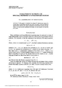
Here we discuss in somewhat more detail Example 25 concerned with a Jacobi matrix having a linear diagonal and constant parallels. For simplicity and with no loss of generality we put α = 1. Our goal is to study how the spectrum of the Jacobi operator J depends on the real parameter w. We treat J as a linear operator-valued function, J = J(w). One may write J(w) = L + wT where L is the diagonal operator with the diagonal sequence λn = n, ∀n ∈ N, and T has all units on the parallels neighboring to the diagonal and all zeros elsewhere. Notice that kT k ≤ 2. We know that J(w) has, for all w ∈ R, a semibounded simple discrete spectrum. Let us enumerate the eigenvalues in ascending order as λs (w), s ∈ N. From the standard perturbation theory one infers that all functions λs (w) are real analytic, with λs (0) = s. Moreover, the functions λs (w) are also known to be even and so we restrict w to the positive real half-axis. In Example 25 we learned that for every w > 0 fixed, the roots of the equation J−z (2w) = 0 are exactly λs (w), s ∈ N. Several first eigenvalues λs (w) as functions of w are depicted in Figure 1. The problem of roots of a Bessel function depending on the order, with the argument being fixed, has a long history. Here we make use of some results derived in the classical paper [6]. Some numerical aspects of the problem are discussed in [15]. For comparatively recent results in this domain one may consult [19] and references therein. In [6] it is shown that  ˆ ∞ −1 dλs (w) = − 2w K0 (4w sinh(t)) exp (2λs (w)t) dt . dw 0 From this relation one immediately deduces a few basic qualitative properties of the spectrum of the Jacobi operator. Proposition 30 (M. J. Coulomb). The spectrum {λs (w); s ∈ N} of the above introduced Jacobi operator, depending on the parameter w ≥ 0, has the following properties. (i) For every s ∈ N, the function λs (w) is strictly decreasing. (ii) If r < s then λr ′ (w) < λs ′ (w). (iii) In particular, the distance between two neighboring eigenvalues λs+1 (w) − λs (w), s ∈ N, increases with increasing w and is always greater than or equal to 1, with the equality only for w = 0. Let us next check the asymptotic behavior of λs (w) at infinity. The asymptotic expansion at infinity of the sth root js (ν) of the equation Jν (x) = 0, with ν being fixed, reads [1, Eq. 9.5.22]
js (ν) = ν − 2−1/3 as ν 1/3 + O ν −1/3 as ν → +∞,

where as is the sth negative zero of the Airy function Ai(x). From here one deduces that
λs (w) = −2w − as w 1/3 + O w −1/3 as w → +∞. 28

Concerning the asymptotic behavior of λs (w) at w = 0, one may use the expression for the Bessel function as a power series and apply the substitution, λs (w) = s − z(w), s = 1, 2, 3, . . .. The solution z = z(w), with z(0) = 0, is then defined implicitly near w = 0 by the equation ∞ X

(−1)m w 2m = 0. m! Γ(m + 1 − s + z(w)) m=0 The computation is straightforward and based on the relation

1 = (−1)m m! z − ψ (0) (m + 1)z 2 + O z 3 , m = 0, 1, 2, 3, . . . , Γ(−m + z)

where ψ (0) is the polygamma function. This way one derives that, as w → 0,
1 (59) λ1 (w) = 1 − w 2 + w 4 + O w 6 , 2
2s 1 w 2s + w 2s+2 + O w 2s+4 , for s ≥ 2. λs (w) = s − (s − 1)!s! (s − 1)(s − 1)!(s + 1)!

The same asymptotic formulas, as given in (59), can also be derived using the standard perturbation theory [17, § II.2]. Alternatively, one may use equivalent formulas for coefficients of the perturbation series derived in [7, 8] which are perhaps more convenient for this particular example. The distance of s ∈ N to the rest of the spectrum of of the diagonal operator L equals 1. The Kato-Rellich theorem tells us that there exists exactly one eigenvalue of J(w) in the disk centered at s and with radius 1/2 as long as |w| < 1/4. The explicit expression for the leading term in (59) suggests, however, that the eigenvalue λs (w) may stay close to s on a much larger interval at least for high orders s. It turns out that actually λs (w) is well approximated by this leading asymptotic term on an interval [0, βs ), with βs ∼ s/e for s ≫ 1. A precise formulation is given in Proposition 33 below. Denote by yk (ν) the kth root of the Bessel function Yν (z), k ∈ N. Let us put  1/(2s) (s − 1)! s! βs := , s ∈ N. π In order to avoid confusion with the usual notation for Bessel functions, the nth truncation of J(w) is now denoted by a bold letter as J n (w).

Lemma 31. The following estimate holds true:   1 1 , ∀s ∈ N. βs < y1 s − 2 2

(60)

Proof. One knows that ν < y1 (ν), ∀ν ≥ 0 [1, Eq. 9.5.2], and in particular this is true for ν = s − 1/2, s ∈ N. On the other hand, the sequence  2s π 1 φs = s− 2−2s (s − 1)! s! 2 29

is readily verified to be increasing, and 1 < φ4 . This shows (60) for all s ≥ 4. The cases s = 1, 2, 3 may be checked numerically. Lemma 32. Denote by χn (w; z) the characteristic polynomial of the nth truncation J n (w) of the Jacobi matrix J(w). If 0 ≤ w ≤ βs for some s ∈ N then z = λs (w) solves the equation wJ2s−z (2w) χ2s−2 (w; z) = 0. (61) χ2s−1 (w; z) − J2s−1−z (2w) Proof. Let {ek ; k ∈ N} be the standard basis in ℓ2 (N). Let us split the Hilbert space into the orthogonal sum ℓ2 (N) = span {ek ; 1 ≤ k ≤ 2s − 1} ⊕ span {ek ; 2s ≤ k}. Then J(w) splits correspondingly into four matrix blocks,   A(w) B(w) J(w) = . C(w) D(w) Here A(w) = J 2s−1 (w), D(w) = J(w) + (2s −1)I, the block B(w) has just one nonzero element in the lower left corner and C(w) is transposed to B(w). By the min max principle, the minimal eigenvalue of D(w) is greater than or equal to 2s − 2w. Since λs (w) ≤ s one can estimate min spec(D(w)) − λs (w) = λ1 (w) − λs (w) + 2s − 1 ≥ s − 2w. We claim that 0 ≤ w ≤ βs implies min spec(D(w)) − λs (w) > 0. This is obvious for s = 1. For s ≥ 2, it suffices to show that βs < s/2. This can be readily done by induction in s. Hence, under this assumption, D(w) − z is invertible for z = λs (w). Solving the eigenvalue equation J(w)vv = zvv one can write the eigenvector as a sum v = x +yy , in accordance with the above orthogonal decomposition. If D(w) − z is invertible then the eigenvalue equation reduces to the finite-dimensional linear system
A − z − B(D − z)−1 C x = 0. (62) One observes that B(D − z)−1 C has all entries equal to zero except of the element in the lower right corner. Using (35) and (15) one finds that this nonzero entry equals wJ2s−z (2w)J2s−1−z (2w)−1 . Equation (61) then immediately follows from (62). Proposition 33. For s ∈ N and 0 ≤ w ≤ βs , one has   πw 2s 1 . 0 ≤ s − λs (w) ≤ arcsin π (s − 1)!s! 30

Proof. We start from Lemma 32 and equation (61). Let us recall from [20, Proposition 30] that  s−k−1 s−1  X
2s − k − 1 2k Y J 2s−1 (w) − s − x) = (−1) x w j 2 − x2 . det (J k j=1 k=0 s

Hence if z ∈ R, |z − s| ≤ 1, then |χ2s−1 (w; z)| ≥ |z − s|

s−1 Y j=1

(63)


j 2 − (z − s)2 .

Since J−s+1/2 (x) = (−1)s Ys−1/2 (x) it is true that for 2w = y1 (s − 1/2) one has λs (w) = s − 1/2. Because of monotonicity of λs (w) one makes the following observation: if 2w ≤ y1 (s − 1/2) then s ≥ λs (w) ≥ s − 1/2. By Lemma 31, if w ≤ βs then 2w ≤ y1 (s − 1/2), and so the estimate (63) applies for z = λs (w). Using also Proposition 4 to express χ2s−2 (w; z) one derives from (61) that   J2s−λ (2w) s − λ w w w |λ − s| ≤ w (64) F , , . . . , J2s−1−λ (2w) 2s − 1 − λ 1−λ 2−λ 2s − 2 − λ

where as well as in the remainder of the proof we write for short λ instead of λs (w). Starting from the equation   w w w , , , . . . = 0, with λ = λs (w), F 1−λ 2−λ 3−λ

and using (4), (15) one derives that, for all k ∈ Z+ , !   k Y w Jk+1−λ (2w) w w (j − λ) F = wk , ,..., . 1 − λ 2 − λ k − λ J (2w) 1−λ j=1

(65)

Combining (64) and (65) we get (knowing that 0 ≤ s − λ ≤ 1/2 for λ = λs (w)) !−1 s−1 s−1 Y Y J2s−λ (2w) 2s−1 (λ − j) (j + s − λ) s−λ≤w . J1−λ (2w) j=1 j=1

But notice that, by expressing the sine function as an infinite product, s−1 s−1 Y Y sin(π(s − λ)) (j + s − λ) = ((s − 1)!)2 (λ − j) π(s − λ) j=1 j=1

Hence

∞  Y j=s

(s − λ)2 1− j2

w 2s−1 J2s−λ (2w) . sin(π(s − λ)) ≤ π ((s − 1)!)2 J1−λ (2w) 31

!−1

.

From (26) one gets, while taking into account that J−λ (2w) = 0, sin(πλ) = πwJλ (2w)J1−λ(2w). In addition, one knows that |Jν (x)| ≤

x ν 1 Γ(ν + 1) 2

provided ν > −1/2 and x ∈ R [1, Eq. 9.1.62]. Hence sin(π(s − λ))2 ≤

π 2 w 4s . ((s − 1)!)2 Γ(2s + 1 − λ)Γ(λ + 1)

Writing λ = s − ζ, with 0 ≤ ζ ≤ 1/2, one has   1 d = −ψ (0) (s + ζ + 1) + ψ (0) (s − ζ + 1) < 0. log dζ Γ(s + ζ + 1)Γ(s − ζ + 1) Thus we arrive at the estimate sin(π(s − λ))2 ≤

π 2 w 4s . ((s − 1)!)2 (s!)2

To complete the proof it suffices to notice that the assumption w ≤ βs means nothing but w 2s / ((s − 1)!s!) ≤ 1, and it also implies that 0 ≤ s − λ ≤ 1/2.

Acknowledgments The authors wish to acknowledge gratefully partial support from the following grants: Grant No. 201/09/0811 of the Czech Science Foundation (P.Š.) and Grant No. LC06002 of the Ministry of Education of the Czech Republic (F.Š.).

References [1] M. Abramowitz, I. A. Stegun: Handbook of Mathematical Functions with Formulas, Graphs, and Mathematical Tables, (Dover Publications, New York, 1972). [2] N. I. Akhiezer: The Classical Moment Problem and Some Related Questions in Analysis, (Oliver & Boyd, Edinburgh, 1965). [3] W. Arveson: C ∗ -Algebras and numerical linear algebra, J. Funct. Anal. 122 (1994) 333-360. [4] B. Beckerman: Complex Jacobi matrices, J. Comput. Appl. Math. 127 (2001) 17-65. 32

[5] T. S. Chihara: An Introduction to Orthogonal Polynomials, (Gordon and Breach, Science Publishers, Inc., New York, 1978). [6] M. J. Coulomb: Sur les zéros de fonctions de Bessel considérées comme fonction de l’ordre, Bull. Sci. Math. 60 (1936) 297-302. [7] P. Duclos, P. Šťovíček, M. Vittot: Perturbation of an eigen-value from a dense point spectrum: an example, J. Phys. A: Math. Gen. 30 (1997) 7167-7185. [8] P. Duclos, P. Šťovíček, M. Vittot: Perturbation of an eigen-value from a dense point spectrum: a general Floquet Hamiltonian, Ann. Inst. H. Poincaré 71 (1999) 241-301. [9] G. Gasper, M. Rahman: Basic Hypergeometric Series, second ed., (Cambridge University Press, Cambridge, 2004). [10] W. Gautschi: Computational aspects of three-term recurrence relations, SIAM Review 9 (1967) 24-82. [11] P. Hartman, A. Winter: Separation theorems for bounded Hermitian forms, Amer. J. Math. 71 (1949) 856-878. [12] E. K. Ifantis, C. G. Kokologiannaki, P. Panagopoulos: Limit points of eigenvalues of truncated unbounded tridiagonal operators, Central Europ. J. Math. 5 (2007) 335-344. [13] E. K. Ifantis, P. Panagopoulos: Limit points of eigenvalues of truncated tridiagonal operators, J. Comput. Appl. Math. 133 (2001) 413-422. [14] E. K. Ifantis, P. D. Siafarikas: An alternative proof of a theorem of Stieltjes and related results, J. Comput. Appl. Math. 65 (1995) 165-172. [15] Y. Ikebe, N. Asai, Y. Miyazaki, DongSheng Cai: The eigenvalue problem for infinite complex symmetric tridiagonal matrices with application, Linear Alg. Appl. 241–243 (1996) 599–618. [16] J. Janas, S. Naboko: Multithreshold spectral phase transition examples in a class of unbounded Jacobi matrices, in Recent Advances in Operator Theory, Oper. Theory Adv. Appl., Vol. 124, (Birkhäuser-Verlag, Basel, 2001), pp. 267-285. [17] T. Kato: Perturbation Theory for Linear Operators, (Springer-Verlag, New York, 1980). [18] M. Malejki: Approximation of eigenvalues of some unbounded self-adjoint discrete jacobi matrices by eigenvalues of finite submatrices, Opuscula Math. 27 (2007) 37-49. [19] E. N. Petropoulou, P. D. Siafarikas, I. D. Stabolas: On the common zeros of Bessel functions, J. Comput. Appl. Math. 153 (2003) 387-393. 33

[20] F. Štampach, P. Šťovíček: On the eigenvalue problem for a particular class of finite Jacobi matrices, Linear Alg. Appl. 434 (2011) 1336-1353. [21] G. Teschl: Jacobi operators and completely integrable nonlinear lattices, (AMS, Rhode Island, 2000). [22] H. S. Wall: Analytic Theory of Continued Fractions, (Chelsea, Bronx NY, 1973).

34

Λ8H w L

8

Λ7H w L

6

Λ6H w L Λ5H w L

4

Λ4 H w L

2

Λ3H w L 1

2

3

4

5

Λ2H w L

-2 -4

Λ1H w L

-6

Figure 1. Several first eigenvalues λs (w) as functions of the parameter w for the Jacobi operator J = J(w) from Example 25, with α = 1.

35

w