The Complexity and Approximation of Fixing ... - Carleton University

The Complexity and Approximation of Fixing Numerical Attributes in Databases Under Integrity Constraints ? Leopoldo Bertossi Carleton University, School of Computer Science, Ottawa, Canada. [email protected]

Loreto Bravo University of Edinburgh, School of Informatics, UK. [email protected]

Enrico Franconi Free University of Bozen–Bolzano, Faculty of Computer Science, Italy. [email protected]

Andrei Lopatenko Google Inc., Mountain View, CA, USA. [email protected]

Abstract Consistent query answering is the problem of characterizing and computing the semantically correct answers to queries from a database that may not satisfy certain integrity constraints. Consistent answers are characterized as those answers that are invariant under all minimally repaired versions of the original database. We study the problem of repairing databases with respect to denial constraints by fixing integer numerical values taken by attributes. We introduce a quantitative definition of database repair, and investigate the complexity of several decision and optimization problems. Among them, DRP: deciding the existence of repairs within a given distance to the original instance, and CQA: deciding consistency of answers to simple and aggregate conjunctive queries under different semantics. We provide sharp complexity bounds, identifying relevant tractable and intractable cases. We also develop approximation algorithms for the latter. Among other results, we establish: (a) The ∆P2 -hardness of CQA. (b) That DRP is MAXSNP-hard, but has a good approximation. (c) The intractability of CQA for aggregate queries for one database atom denials (plus built-ins), and also that it has a good approximation. Key words: Integrity constraints, Inconsistent databases, Consistent query answering, Database repairs

Preprint submitted to Elsevier Science

1

Introduction

Integrity constraints (ICs) are used to impose semantics on a database. In this way, the database becomes an accurate model of an application domain. Database management systems or application programs enforce the satisfaction of the ICs by either rejecting undesirable updates or by executing additional compensating actions. However, there are many situations where we need to interact with a database that is inconsistent wrt certain desirable ICs. An important problem in database research consists in characterizing and retrieving consistent data from inconsistent databases, in particular, consistent answers to queries [4]. From the logical point of view, consistently answering a query on an inconsistent database amounts to evaluating the truth of a formula against a particular class of first-order relational structures [2]. This process is quite different from usual truth or query evaluation on a single structure, namely the relational database at hand. In our case, the class under consideration is formed by alternative instances that are consistent, i.e. satisfy the ICs, and minimally differ from the original database, the so-called repairs of the latter. What is consistently true in the original instance corresponds to what is classically true of all repairs. Obviously, the notion of repair depends upon particular notions of difference between database instances and minimality. Certain database applications, such as census, demographic, financial, and experimental data, contain quantitative data usually associated to nominal or qualitative data. For example, the number of children associated to a household identification code (or address); and the measurements associated to a sample identifier. Often this kind of data contains errors or mistakes with respect to certain semantic constraints. For example, a census form for a particular household may be considered incorrect if the number of children is negative; or if the age of a mother is less than those of her offsprings. These restrictions can be expressed with denial integrity constraints, which prevent attributes from taking certain combinations of values [18]. Other restrictions may be expressed with aggregation ICs. For example, the maximum concentration of certain toxin in a sample may not exceed a known threshold; or the number of married men and married women must be the same. Inconsistencies in numerical data can be resolved by changing individual attribute values, while keeping values in the keys, e.g. without changing the household code, the number of children is decreased considering the admissible values. More precisely, we consider the problem of fixing integer numerical data wrt certain constraints while (a) keeping the attribute values in the keys ? Dedicated to the memory of Alberto Mendelzon. Our research on this topic started with conversations with him. Alberto was always generous with his time, advice and ideas.

2

of the relations, and (b) minimizing the quantitative global distance between the original and modified instances. Since the problem may admit several global solutions, each of them involving possibly many individual changes, we are interested in characterizing and computing data and properties that remain invariant under any of these repair processes. We concentrate on denial constraints; and conjunctive queries, with or without aggregation. Database repairs have been studied in the context of consistent query answering (CQA), i.e. the process of obtaining the answers to a query that are consistent wrt a given set of ICs [2] (cf. [4,5,13] for surveys). An answer to a query is consistent if it can be obtained as a standard answer to the query from every possible repair. In most of the research on CQA, a repair is a new instance that satisfies the given ICs, but differs from the original instance by a minimal set, under set inclusion, of (completely) deleted or inserted tuples. Changing the value of a particular attribute can be modelled as a deletion followed by an insertion, but this may not correspond to a minimum repair. In certain applications it may make more sense to correct (update) values in certain numerical attributes only. This requires a new definition of repair that considers: (a) the quantitative nature of individual changes, (b) the association of the numerical values to other key values; and (c) a quantitative distance between database instances. We consider fixable attributes that take integer values. Only in these fixable attributes we allow for changes of values with the purpose of restoring consistency. In consequence, obtaining a repair becomes a numerical constraint satisfaction problem, where the constraints are given by the denials. The additional requirement in this problem is that the solutions, i.e. instances, should stay close to the initial instance. Example 1 Consider a network traffic database D storing flow measurements of links in a network. This network has two types of links, labelled 0 and 1, with maximum flows 1000 and 1500, resp. The following database D is inconsistent wrt this constraint on the values that flows may take. Traffic Time 1.1 1.1 1.3

Link a b b

Type Flow 0 1100 1 900 1 850

Under the tuple and set oriented semantics of repairs [2], there is a unique repair, namely deleting tuple Traffic(1.1, a, 0, 1100). However, we have two options that may make more sense than deleting the flow measurement, namely updating the violating tuple to Traffic(1.1, a, 0, 1000) or to Traffic(1.1, a, 1, 1100). These alternatives would satisfy the implicit requirement that the numbers should not change too much. 2 In order to define a sensible distance function, for comparing alternative repairs to the original instance, we think that the numerical nature and the

3

magnitude of these changes have to be considered. In this paper we start from the assumption that keeping the overall and absolute variation of values small and in balance is something desirable. A natural and usual way to achieve this goal consists in minimizing the square distance between the initial instance and a repair. For more flexibility, we allow for different weights to be assigned to the fixable attributes, and these weights are brought into the distance formula. In the same spirit, other distances between database instances, as an alternative to the Euclidean or L2 distance that we investigate in this paper, could be considered (c.f. Section 7.4). Specific repairs and approximations may be different under other distance functions, e.g. the “city distance” L1 (the sum of absolute differences), but the general (in)tractability and approximation results remain. The problem of attribute-based correction of census data forms is addressed in [18] using disjunctive logic programs with stable model semantics. Several underlying and implicit assumptions that are necessary for that approach to work are made explicit and used here, extending the semantic framework of [18]. However, in that work the numerical nature of some attributes is not brought into the model, and the distance just counts the number of changes, no matter how big or small they are. Update-based repairs for restoring consistency are also studied in [34], where changing values in attributes in a tuple is made a primitive repair action. Semantic and computational problems around CQA are analyzed from this perspective. However, peculiarities of changing numerical attributes are not considered, and more importantly, the distance between databases instances used in [34,35] is based on set-theoretic homomorphisms, but is not quantitative, as in this paper. We provide semantic foundations for repairs that are based on changes on numerical attributes in the presence of key dependencies and wrt denial constraints, while keeping the numerical distance to the original database to a minimum. This framework introduces new challenging decision and optimization problems, and many algorithmic and complexity theoretic issues. We concentrate in particular on the “Database Repair Problem” (DRP) of determining the existence of a repair at a distance not greater than a given bound. In particular, we consider the problems of construction and verification of such a repair. These problems are highly relevant for large inconsistent databases. For example, solving DRP can help us find the minimum distance from a repair to the original instance. This information can be used to prune impossible branches in the process of materialization of a repair. The CQA problem of deciding the consistency of query answers is studied wrt decidability, complexity, and approximation under several alternative semantics. We prove that DRP is NP-complete for denial constraints, which are enough to capture census like applications. CQA belongs to ΠP2 and becomes ∆P2 -

4

hard. For a particular, simple, but relevant class of denials we get tractability of CQA for a large and relevant class of non aggregate queries. For the same class of denials, simple aggregations based on acyclic conjunctive queries easily lead to intractability of CQA. Wrt approximation, we prove that DRP is MAXSNP -hard in general; and for a relevant subclass of denials, we provide a polynomial time approximation within a constant factor. All the algorithmic and complexity results, unless otherwise stated, refer to data complexity [1], i.e. to the size of the database that here includes a binary representation for numbers. For complexity theoretic definitions and classical results we refer to [29]. Moving to the case of real numbers would certainly bring new issues that would require different approaches. They are left for ongoing and future research. Actually, it would be natural to investigate them in the richer context of constraint databases [25]. For databases like those we are considering here, aggregation constraints may also be relevant. Here we briefly study the DRP and CQA problems when repairs have to satisfy aggregation constraints. It turns out that both problems become undecidable when both the instance and the constraints are part of the input. This paper is structured as follows. Section 2 introduces basic definitions. Section 3 presents the notion of database repair, several semantics for the notion of consistent answer to a query; and some relevant decision problems. Section 4 investigates their complexity. In Section 5, approximation algorithms for the problem of finding the minimum distance to a repair are studied. We obtain negative results for the general case, but a good approximation for the relevant class of local denial constraints. Section 6 investigates tractability of CQA for conjunctive queries and denial constraints containing one database atom plus built-ins. Section 7 contains extensions of the main framework, like a brief analysis of repairs that have to satisfy certain statistical conditions, the above mentioned results around aggregation constrains, and a discussion of alternative distances. Section 8 presents some conclusions and refers to related work.

2

Preliminaries

Consider a relational schema Σ = (U, R, B), with domain U that includes Z,R a set of database predicates, B a set of built-in predicates. If a predicate R ∈ R has arity n ≥ 1, each of its n arguments has associated a unique attribute name that is not shared with other argument positions of database predicates in the schema. This is not an essential restriction, but it will make the formulation of some definitions much simpler. The set of attribute names (we will simply 5

call them attributes) in the schema is denoted with A. According to this, we usually denote a database predicate with R(A1 , . . . , An ), with each Ai ∈ A. A(R) denotes the set of attributes of R. It holds A(R) ⊆ A. Each attribute A has a domain that is a subset of U, where it can take values. Different attributes may share the same domain and make take the same values. Numerical attributes are those that have domain Z. With denial constraints, we can make a numerical attribute take values in a subset of Z, e.g. in N or {0, 1}. For the latter case, we can use denial constraints like ∀x, y¬(R(x, y) ∧ x < 0), ∀x, y¬(R(x, y) ∧ x > 1). A database instance is a finite collection D of database tuples, i.e. of ground atoms R(¯ c), with R ∈ R and c¯ a finite sequence of constants in U. If R(A1 , . . . , An ) ∈ R, t = R(c1 , . . . , cn ) ∈ D, and S = (Ai1 , . . . , Aik ) is a subsequence of (A1 , . . . , An ), then t[Ai1 , . . . , Aik ] denotes the projection of tuple t on S, i.e. (ci1 , . . . , cik ). For k = 1, we simple write t(Ai ) = ci . There is a set F ⊆ A containing all the fixable attributes, those that take values in Z and are allowed to be fixed. Attributes outside F are called rigid. F need not contain all the numerical attributes, that is, we may also have rigid numerical attributes. More precisely, each predicate R ∈ R has a set of fixable attributes, denoted by F(R). It holds F(R) ⊆ F . We also have a set K of key constraints expressing that predicates R ∈ R have a primary key KR , with KR ⊆ (A(R) r F(R)). Later on (cf. Definition 2), we will assume that K is satisfied both by the initial instance D, denoted D |= K, and its repairs. In this sense, we say the elements of K are hard. Since F(R) ∩ KR = ∅, values in rigid attributes cannot be changed in a repair process. In addition, there may be a separate set IC of flexible ICs that may be violated, and it is the job of a repair to restore consistency wrt them (while still satisfying K). A linear denial constraint [25] has the form ∀¯ x¬(A1 ∧ . . . ∧ Am ), where the Ai are database atoms (i.e. with predicate in R), or built-in atoms of the form xθc, where x is a variable, c is a constant, and θ ∈ {=, 6=, , ≤, ≥}, or of the form x = y. If x 6= y is allowed, we call them extended linear denials. We assume that all the constants appearing in ICs belong to the domain U. In a constraint, x¯ denotes the sequence of variables, say x¯ = x1 , . . . , xn , that appear in the conjunction of atoms. Since the order in which the variables appear in the quantification does not matter, we usually identify x¯ with the set formed by its variables, say {x1 , . . . , xn }. Furthermore, in denials we usually replace ∧ by a comma, and sometimes we use ∀ for the whole prefix of universal quantifications. Unless otherwise stated, all the flexible ICs in this paper are denial constraints; and sets of denials are always finite. Example 2 The following are linear denials: (a) No customer is younger than 21: ∀Id , Age, Income, Status¬(Customer (Id , Age, Income, Status), Age < 21). (b) No customer with income less than 60000 has “silver” status: ∀Id , Age, Income, Status¬(Customer (Id , Age, Income, Status), Income < 60000, Status 6

= silver ). (c) The constraint in Example 1, i.e. ∀T , L, Type, Flow ¬(Traffic(T, L, Type, Flow ), Type = 0, Flow > 1000). 2 In this example, in order to make the intuitive contents of a denial constraint more clear, we have used the attribute names as variables. Sometimes this practice will allow us to simplify the formulation of some definitions and results. This can always be done, by introducing extra versions of the attributes names if necessary; versions that are not shared by other attribute names. For example, for the predicate R(A, B), the denial ∀x, y, z¬(R(x, z), R(y, z), z = 1) can be rewritten as ∀A, A0 , B¬(R(A, B), R(A0 , B), B = 1). We will consider aggregate queries containing the aggregation functions sum, count, or average. More precisely, an aggregate conjunctive query has the form q(x1 , . . . xm ; agg(z)) ← B(x1 , . . . , xm , z, y1 , . . . , yn ), where agg is an aggregation function. The non aggregate matrix (NAM) of the aggregate query is given by q 0 (x1 , . . . xm ) ← B(x1 , . . . , xm , z, y1 , . . . , yn ), which is a usual firstorder (FO) conjunctive query with built-in atoms. In the query predicate q, the aggregation attribute (or variable) z does not appear among the xi . We use the set semantics for aggregate queries. An aggregate conjunctive query is cyclic (acyclic) if its NAM is cyclic (acyclic) [1]. Example 3 q(x, y, sum(z)) ← R(x, y), Q(y, z, w), w 6= 3 is an aggregate conjunctive query, with aggregation attribute z. Each answer (x, y) to its NAM, i.e. to q(x, y) ← R(x, y), Q(y, z, w), w 6= 3, is expanded to (x, y, sum(z)) as an answer to the aggregate query. sum(z) is the sum of all the values for z having a w, such that (x, y, z, w) makes R(x, y), Q(y, z, w), w 6= 3 true. In the database instance D = {R(1, 2), R(2, 3), Q(2, 5, 9), Q(2, 6, 7), Q(3, 1, 1), Q(3, 1, 5), Q(3, 8, 3)} the answer set for the aggregate query is {(1, 2, 5 + 6), (2, 3, 1 + 1)}. In this example, the aggregate query is a group-by query, because the query predicate has free variables (x and y). 2 An aggregate comparison query is a sentence of the form q(agg(z)) ∧ agg(z)θk, where q(agg(z )) is the head of a scalar aggregate conjunctive query (i.e. with no free variables, or equivalently, without group-by), θ is a comparison operator, and k is an integer number. For example, the following is an aggregate comparison query asking whether the aggregated value obtained via q(sum(z)) is greater than 5: Q : q(sum(z)) ∧ sum(z) > 5, with q(sum(z)) ← R(x, y), Q(y, z, w), w 6= 3. We can see that aggregate comparison queries are boolean, i.e. they have a true or false answer in a database instance. An aggregate comparison query q(agg(z)) ∧ agg(z)θk is (a)cyclic if the NAM of the query that defines q(agg(z)) is (a)cyclic.

7

3

Least Squares Repairs

When we update numerical values to restore consistency, it is desirable to make the smallest overall variation of the original values, while considering the relative relevance or specific scale of each of the fixable attributes. Since the original instance and a repair will share the same rigid values (cf. Definition 2), we can use them to compute variations in the numerical values. Now, we make this idea more precise. We say that instances D, D0 over Σ are rigid-comparable if for every tuple t = R(¯ c) ∈ D, for some R ∈ R, there is a unique tuple t0 = R(¯ c0 ) ∈ D0 such that t[A(R) r F(R)] = t0 [A(R) r F(R)], and viceversa. In this case, we write t0 = m(t), indicating that tuple t0 ∈ D0 is the corresponding version of t ∈ D, possibly modified at its fixable attributes. That is, tuples t and t0 coincide on the values of their rigid attributes. Definition 1 For rigid-comparable instances D and D 0 over schema Σ, their P square distance is ∆α¯ (D, D 0 ) = t∈D,A∈F αA · (t(A) − m(t)(A))2 , and α ¯ = (αA )A∈F . 2 Definition 2 Let D, D0 be instances over the same schema Σ, such that D |= K and D0 |= K; and IC be a set of flexible ICs. D0 is a repair for D wrt IC if: (a) D, D0 are rigid-comparable; and (b) D0 |= IC. A least squares repair (LS-repair) for D is a repair D0 that minimizes the square distance ∆α¯ (D, D0 ) over all the instances that satisfy (a) and (b). 2 The conditions in this definition make D and D0 rigid-comparable, and Definition 1 can be applied. In general, we are interested in LS-repairs, but (not necessarily minimum) repairs will be useful auxiliary instances. Example 4 (example 1 cont.) R = {Traffic}, A = {T ime, Link, T ype, F low}, KTraffic = {T ime, Link}, F = {T ype, F low}, with weights α ¯ = −5 (10 , 1), resp. A repair of the original instance D is D1 = {Traffic(1.1, a, 0, 1000), Traffic(1.1, b, 1, 900), Traffic(1.3, b, 1, 850)}. In this case, m(Traffic(1.1, a, 0, 1100)) = Traffic(1.1, a, 0, 1000), etc. Another repair is D2 = {Traffic(1.1, a, 1, 1100), Traffic(1.1, b, 1, 900), Traffic(1.3, b, 1, 850)}. The distances are ∆α¯ (D, D1 ) = 1002 × 10−5 = 10−1 and ∆α¯ (D, D2 ) = 12 × 1. D1 is the only LS-repair. 2 The coefficients αA can be chosen in many different ways depending on factors like relative relevance of attributes, actual distribution of data, measurement scales, etc. In the rest of this paper we will assume, for simplification, that αA = 1 for all A ∈ F , and ∆α¯ (D, D 0 ) will be simply denoted by ∆(D, D 0 ). Example 5 Database D has predicates Client(ID, A, C ), with attributes for identification (the key), age and credit line of the client; and Buy(ID1 , I , P ), with key {ID1 , I} and containing clients buying items at certain prices. There

8

are two denial ICs ic 1 : ∀ID1 , P, A, C¬( Buy(ID1 , I, P ), Client(ID, A, C), ID1 = ID, A < 18, P > 25) and ic 2 : ∀ID, A, C¬( Client( ID, A, C), A < 18, C > 50), requiring that people younger than 18 cannot spend more than 25 on one item nor have a credit line higher than 50 in the store. The following table shows the database contents. We added an extra column to be able to refer to the tuples. D:

Client

ID 1 2 3

A 15 16 60

C 52 51 900

Buy t1 t2 t3

ID1 1 1 3

I CD DVD DVD

P 27 26 40

t4 t5 t6

We can see that ic 1 is violated by {t1 , t4 } and {t1 , t5 }, and ic 2 by {t1 } and {t2 }. Assuming that αA = αC = αP = 1, we have two LS-repairs, D0 , D00 , at a distance 10 from the original instance. D0 :

D00 :

Client

Client

ID 1 2 3

A 15 16 60

C 50 50 900

ID 1 2 3

A 18 16 60

C 52 50 900

Buy t01 t2 0 t3 Buy 00

t1 t2 00 t3

ID1 1 1 3

I CD DVD DVD

P 25 25 40

t4 0 t5 0 t6

ID1 1 1 3

I CD DVD DVD

P 27 26 40

t4 t5 t6

2 In this example, it was possible to obtain LS-fixes by performing direct, local changes in the original conflictive tuples alone. No new, intermediate inconsistencies are introduced in the repair process. The following example shows that this may not be always the case. Example 6 Consider a database D with relations P (A, B, C) and Q(D, E) with KP = {A}, KQ = {D} and F = {B, C, E}; and linear denials ic 1 : ∀x, y, z, w¬(P (x, y, z), Q(x, w), y > 3, w > 5) and ic 2 : ∀x, y, z¬(P (x, y, z), y < 5, z < 4). The following instance is inconsistent, because {t1 , t2 } violates ic 1 . P

A a

B 6

C 1

Q t1

D a

E 9

t2

If we tried to find a repair by making the smallest change that restores consistency, t1 (B) would be replaced by 3 (the alternative of replacing t2 (E) by 5 is more expensive): P

A a

B 3

C 1

Q t01

D a

E 9

t2

This new instance is still inconsistent since {t01 } violates ic 2 . Now, if we tried

9

to solve this new inconsistency by making the smallest variation, t01 (B) would be replaced by 5, which violates ic 2 again. Actually, the only LS-repair is: P

A a

B 6

C 1

Q t1

D a

E 5

t02

We can see that new inconsistencies can be introduced by local changes, and that an LS-repair is not necessarily a sequence of minimum local changes. 2 The numerical values in the denial constraints define threshold values that may determine their satisfaction by a database instance. Definition 3 Let IC be a set of extended linear denials. The set of borders of IC is Borders(IC) = {c | there is ic ∈ IC and a variable x in ic, such that x appears in the position of fixable attribute in a predicate in ic and either (x < c), (x > c), (x ≤ c − 1), (x ≥ c + 1), (x = c − 1), (x = c + 1), or (x 6= c) appears as a comparison in ic}. 2 When comparisons of the type x = y or x 6= y, and joins involve only rigid attributes, the built-in atoms in extended linear denials determine a solution space for repairs as an intersection of semi-spaces. LS-repairs can be found taking values from the borders of the ICs (cf. previous examples). However, if comparisons of the type x = y or x 6= y, or joins in the denials involve fixable attributes, then the attribute values in LS-repairs can be found in intervals around borders, as defined by the denials, and around values in tuples of the inconsistent database. Lemma 1 Let D0 be an LS-repair of D wrt a set IC of extended linear denial constraints. Let a = |A|. For each tuple t ∈ D0 and fixable attribute A of t, it holds t(A) ∈ [v − a, v + a], for some integer v in a tuple in D, or t(A) ∈ [c−a, c+a], for some c ∈ Borders(IC). Furthermore, if IC is such that equalityand 6=-atoms between attributes, and joins involve only rigid attributes, then either t(A) = m−1 (t)(A) or t(A) ∈ Borders(IC).1 2 If there are equalities, non-equalities or joins involving fixable attributes, the LS-repairs can take values that are not borders nor values from the inconsistent database. The following examples show such cases and illustrate Lemma 1. Example 7 Consider a predicate T (X, Y ), with only Y fixable, and the instance D = {T (3, 3)}, which is inconsistent wrt IC = {∀x, y¬(T (x, y), x = y)}. In this case, Borders(IC) = ∅. There are two LS-repairs: D0 = {T (3, 2)} and D00 = {T (3, 4)}. The values for attribute Y in both LS-repairs can be found in the interval [v − |A|, v + |A|], with v = 3 and |A| = 2. 2 Example 8 Consider a predicate R(A, B, C, D), with only B fixable, and a set of ICs IC = {∀x, y, z, w¬(R(x, y, z, w), y < 6), ∀x, y, z, w¬(R(x, y, z, w), 1

We recall that m(t) ∈ D0 , with D0 a repair of D, is the tuple that results from modifying t ∈ D.

10

y = z), ∀x, y, z, w ¬(R(x, y, z, w), z = w)}. The instance D = {t} with t : R(1, 5, 6, 7) is inconsistent. Here, Borders(IC) = {6}. The inconsistency wrt the first IC can be solved by changing t(B) from 5 to 6. This new value violates the second constraint. So now, to stay as close as possible to the original instance, we replace t(B) by 7. This value now violates the third constraint. By increasing the value by one once more, we get an LS-repair D0 = {R(1, 8, 6, 7)}. The value taken by B is a border value plus 2. 2 Proof of Lemma 1 First we will concentrate in the case where IC is such that the attributes participating in equality atoms between attributes or in joins are all rigid. Let us assume, by contradiction, that there exists a tuple t ∈ D0 and a fixable attribute A, for which t(A) = k and k 6= m(t)(A) and k 6∈ Borders(IC). Without loss of generality, assume that k < m(t)(A). Let D00 be the same as D0 except that t(A) is changed from k to k − 1. Since k 6∈ Borders(IC), no new inconsistencies can be added since the built-ins that were (or were not) satisfied before, will continue in the same state. Thus, D00 also satisfies IC and is rigid-comparable to D. However, D00 is closer to D than D0 . Thus, D0 is not an LS-repair. We have a contradiction. In the general case, integrity constraints may have fixable attributes participating in (non-)equality atoms between attributes or in joins. In this case, the value of such an attribute in a tuple might be changed to satisfy a constraint, so that the equality does not hold. As before, we assume there exists an LSrepair D0 and an attribute A such that t(A) = k and k is not in [v − a, v + a] for each numerical value v in a tuple in D, nor in [c − a, c + a] for each c ∈ Borders(IC). In a similar way as in the proof for the case with equalities and joins between rigid attributes, a contradiction can be reached. 2 It is easy to construct examples with an exponential number of repairs. For the kind of repairs and ICs we are considering, it is possible that no repair exists, in contrast to [2,3], where, if the set of ICs is consistent as a set of logical sentences, a repair for a database always exists. Example 9 R(A, B) has key A, and B is fixable. IC = {∀x1 , x2 , y ¬(R(x1 , y), R(x2 , y), x1 = 1, x2 = 2),∀x1 , x2 , y ¬(R(x1 , y), R(x2 , y), x1 = 1, x2 = 3), ∀x1 , x2 , y ¬(R(x1 , y), R(x2 , y), x1 = 2, x2 = 3), ∀x, y ¬(R(x, y), y> 3), ∀x, y ¬( R(x, y), y < 2)} is consistent. The first three ICs force attribute B to be different in every tuple. The last two ICs require 2 ≤ B ≤ 3. The inconsistent database D = {R(1, −1), R(2, 1), R(3, 5)} has no repair. 2 Proposition 1 If D has a repair wrt IC, then it also has an LS-repair wrt IC. Proof: Let ρ be the square distance between D and a repair D0 according to Definition 1. The circle of radius ρ around D containing instances over the same schema that share the rigid attribute values with D intersects the non empty “consistent” region that contains the database instances with the

11

same schema and rigid values as D and satisfy IC. All the instances within that circle have their fixable numerical values bounded in absolute value by a fixed function of ρ and the fixable values in D. In consequence, the circle has a finite number of instances, and the distance takes a minimum in the consistent region. 2 4

Decidability and Complexity

In applications where repairs are based on changes of numerical values, computing concrete repairs is a relevant problem. In databases containing census forms, correcting the latter before doing statistical processing is a common problem [18]. In databases with experimental samples, we can fix certain erroneous quantities as specified by linear ICs. In these cases, the repairs are relevant objects to compute explicitly, which contrasts with CQA [2], where the main motivation for introducing repairs is to formally characterize the notion of a consistent answer to a query, as an answer that persists under all possible repairs. In consequence, we now consider some decision problems related to existence and verification of LS-repairs, and to CQA under different semantics. Definition 4 For an instance D and a set IC of ICs: (a) Rep(D, IC) = {D0 | D0 is an LS-repair of D wrt IC}, the repair checking problem. (b) Rep(IC) = {(D, D0 ) | D0 ∈ Rep(D, IC)}. (c) NE (IC) = {D | Rep(D, IC) 6= ∅}, for non empty set of repairs, i.e. the problem of checking existence of LS-repairs. (d) DRP (IC) ={(D, k) | there is D0 ∈ Rep(D, IC) with ∆(D, D0 ) ≤ k}, the database repair problem, i.e. the problem of checking existence of LS-repairs within a given positive distance k. (e) DROP (IC) is the optimization problem of finding the minimum distance from an LS-repair wrt IC to a given input instance. 2 Notice that, by Proposition 1, DRP (IC) could also be defined as {(D, k) | there is a repair D0 of D with ∆(D, D0 ) ≤ k}. Definition 5 Let D be a database, IC a set of ICs, and Q a conjunctive query. 2 (a) A finite sequence c¯ of constants in U is a consistent answer to Q(¯ x) under the: (a1) skeptical semantics if for every D0 ∈ Rep(D, IC), 0 D |= Q(¯ c). (a2) brave semantics if there exists D0 ∈ Rep(D, IC) with D0 |= Q(¯ c). 3 (a3) majority semantics if |{D0 | D0 ∈ Rep(D, IC) and D0 |= Q(¯ c)}| 0 0 0 > |{D | D ∈ Rep(D, IC) and D 6|= Q(¯ c)}|. (b) That c¯ is a consistent answer to Q in D under semantics S is denoted by 2 3

Whenever we say “conjunctive query”, we mean a non aggregate query. Skeptical and brave semantics are aka. certain and possible semantics, resp.

12

D |=S Q[¯ c]. If Q is boolean (i.e. a sentence) and D |=S Q, we say that yes is a consistent answer, meaning that Q is true in the repairs of D as prescribed by semantics S. CA(Q, D, IC, S) is the set of consistent answers to Q in D wrt IC under semantics S. For a boolean Q, if CA(Q, D, IC, S) 6= {yes}, CA(Q, D, IC, S) = {no}. (c) CQA(Q, IC, S) = {(D, c¯) | c¯ ∈ CA(Q, D, IC, S)} is the decision problem of consistent query answering, i.e. of checking consistent answers. 2 In the literature on consistent query answering, the notion of consistent answer and the CQA problem usually refer to the skeptical semantics. Proposition 2 NE (IC) can be reduced in polynomial time to the complements of CQA(False, IC, Skeptical ) and CQA(True, IC, Majority), where False, True are ground queries that are always false, resp. true. Proof: First for the skeptical semantics. Given a database instance D, consider the instance (D, no) for CQA(False, IC, Skeptical ), corresponding to the question “Is there an LS-repair of D wrt IC that does not satisfy False?” has answer yes iff the class of LS-repairs of D is empty. For the majority semantics, for the instance (D, no) for CQA(True, IC, Majority), corresponding to the question “Is it not the case that the majority of the LS-repairs satisfy True?”, we get answer yes iff the set of LS-repairs is empty. 2 In Proposition 2, it suffices for queries True, False to be true, resp. false, in all instances on the same schema as the input database. The former can be represented by (yes) ←, a query with empty body; and the latter by (yes) ← R(. . . , x, . . .), x = 1, x = 2, where variable x corresponds to a numerical attribute. Theorem 1 For every fixed set IC of linear denials: (a) Deciding if for an instance D there is a repair D0 with ∆(D, D0 ) ≤ k, with positive integer k that is part of the input, is in NP . (b) There is a fixed set IC of denials for which DRP (IC) is NP -complete. Proof: (a) First of all, we notice that a linear denial with implicit equalities, i.e. occurrences of a same variable in two different database atoms, e.g. ∀x, y, z¬(R(x, y), Q(y, z), z > 3), can be replaced by its explicit version with explicit equalities, e.g. ∀x, y, z, w¬(R(x, y), Q(w, z), y = w, z > 3). Let n be the number of tuples in the database, and l be the number of attributes that appear in built-in predicates in the explicit versions of the ICs. For example, consider the denial ∀x, y, z¬(P (x, y), Q(z, x), y > 2). The explicit version is ∀x, y, z, w¬(P (x, y), Q(z, w), y > 2, x = w) and l would be 3 (for x, y, w). Notice that, by Proposition 1, there is a repair at a distance not greater than k iff there is an LS-repair at a distance not greater than k.

13

If there exists an LS-repair D0 with ∆(D, D0 ) ≤ k, then no value in a fixable 0 attribute √ for a tuple in D differs from its corresponding value in D by more than k. In consequence, the size of an LS-repair may not differ from the original instance by more than l × n × bin(k)/2, where bin(k) is the size of the binary representation of k. Thus, the size of an LS-repair is polynomially bounded by the size of D and k. Since we can determine in polynomial time if D0 satisfies the ICs and if the distance is smaller than k, we obtain the result. (b) Membership: According to Proposition 1, there is an LS-repair at a distance ≤ k iff there is a repair D0 at a distance ≤ k. We use part (a) of this proposition. Hardness: We can reduce Vertex Cover to DRP (IC0 ) for a fixed set of denials IC0 . Given a graph instance (V, E), k for VC, consider a database schema with a binary predicate E(X, Y ) with key {X, Y } for the edges of the graph, and a predicate V (X1, Chosen), with key X1 that takes vertices as values. Attribute Chosen is the only fixable attribute. The original database D contains the tuples E(e1 , e2 ), E(e2 , e1 ) for {e1 , e2 } ∈ E, and the tuples V (v, 0) for v ∈ V. The constraint IC : ∀x, y, c1 , c2 ¬(E(x, y) ∧ V (x, c1 ) ∧ V (y, c2 ) ∧ c1 < 1 ∧ c2 < 1) expresses that for any edge, at least one of the incident vertices is covered. A vertex cover of size k exists iff there exists an LS-repair of D wrt IC at a distance ≤ k. The encoding is polynomial in the size of the original graph. 2 By Proposition 1, there is a repair for D wrt IC at a distance ≤ k iff there is an LS-repair at a distance ≤ k. So, a test for the former, that is analyzed in Theorem 1(a), can be used for the latter. Actually, if we happen to know, e.g. by using the test in 1(a), that there is a repair at a distance ≤ k, then the minimum distance between D and a repair (i.e. the distance between D and any LS-repair) can be found by binary search in the distance interval [0, k] in log(k) steps, using at each of them the test in Theorem 1(a). If an LS-repair exists, its square distance to D is polynomially bounded by the size of D (cf. Lemma 2 below). Since D and a repair have the same number of tuples, only the size of their values in a repair matter, and they are constrained by a fixed set of linear denials and the condition of minimality. Lemma 2 Given a database D and a set of extended denials IC, the size of an LS-repair D0 is polynomial in the size of D and the numerical constants in the ICs. This is also true if D0 is a repair obtained from D by replacing values of fixable attributes by values at the intervals around numerical values in D or the borders determined by the ICs (according to Lemma 1). Proof: The proof of the first claim follows immediately from: (a) The LSrepair D0 has the same number of tuples as D, and (b) By Lemma 1, in an LS-repair, the value for each attribute and in each tuple falls in an interval of the form [c − |A|, c + |A|], where c is either a value of D or a border. For the

14

second claim, the proof is similar, since D0 has the same number of tuples as D. 2 Theorem 2 For a fixed set IC of extended linear denials: (a) The problem NE (IC) of deciding if an instance has an LS-repair wrt IC is NP -complete, and (b) CQA under the skeptical and the majority semantics is coNP -hard. Proof: (a) For hardness, it suffices to consider linear denials. We reduce 3Colorability to NE (IC0 ), for a fixed set IC0 of ICs. Let G = (V, E) be an undirected graph with set of vertices V and set of edges E. Consider the following database schema, instance D, and set IC0 of ICs: 1. Predicate V ertex(Id , Red , Green, Blue), with key Id , and domain N for the last three attributes, actually the only three fixable attributes in the schema. For each v ∈ V, we have Vertex (v, 0, 0, 0) in D (and no other Vertex tuple in D). 2. Predicate Edge(Id1 , Id2 ), with no fixable attributes. For each e = {v1 , v2 } ∈ E, Edge(v1 , v2 ), Edge(v2 , v1 ) ∈ D. 3. Predicate Tester (Red1 , Green1 , Blue1 ), with no fixable attributes, and extension Tester (1, 0, 0), Tester (0, 1, 0), Tester (0, 0, 1) in D. 4. Integrity constraints: ∀i, x, y, z¬(Vertex (i, x, y, z), x < 1, y < 1, z < 1); ∀i, x, y, z¬(Vertex (i, x, y, z), x > 1) (the same for y, z); ∀i, x, y, z¬(Vertex (i, x, y, z), x = 1, y = 1, z = 1); ∀i, x, y, z¬(Vertex ( i, x, y, z), x = 1, y = 1); etc. ∀i, j, x, y, z¬(Vertex (i, x, y, z), Vertex (j, x, y, z), Edge(i, j), Tester (x, y, z)). If there is an LS-repair wrt IC0 of the generated instance, then the graph is 3-colorable. If the graph is 3-colorable, then there is a consistent instance with the same rigid values as the original instance. Thus, by Proposition 1, there is an LS-repair. The reduction is polynomial in the size of the graph. Now we prove membership. By Proposition 1 and Lemma 1, the existence of a repair is equivalent to the existence of an LS-repair; and the latter is equivalent to the existence of a repair that has its modified fixable values taken at the intervals around the borders of the corresponding attributes or around the values in the tuples of D (cf. Lemma 1). So, we can concentrate on the latter problem. An NP algorithm for this problem is as follows: (1) For the positive cases D, guess a witness, i.e. a repair D0 of D that shares the values of non fixable attributes with D, and the modified values of the fixable attributes taken from intervals of the form [c − |A|, c + |A|], for c a value in D or a border. (2) Check that D, D0 are rigid-comparable. (3) Check that D0 satisfies the ICs. This test is polynomial in the size of D, D0 . By Lemma 2, the size of D0 is polynomial in the size of D. (b) coNP -hardness follows from Proposition 2 and part (a).

15

2

For hardness in (a) and (b) in Theorem 2, linear denials suffice. Membership in (a) can be obtained for any fixed finite set of extended denials. Theorem 3 For a fixed set IC of linear denials: (a) The problem Rep(IC) of checking if an instance is an LS-repair is coNP -complete, and (b) CQA under skeptical semantics is in ΠP2 , and, for ground atomic queries, ∆P2 -hard. Proof: (a) We reduce 3-SAT’s complement to Rep(IC) for a fixed schema and set IC of denials. We have a predicate Lit(l, ¯l) whose extension stores complementary literals (only), e.g. Lit(p, ¬p) when p is one of the variables in the instance Φ of SAT. Also a predicate Cl for tuples of the form Cl (ϕ, l, k), where ϕ is a clause of Φ (we assume, wlog. that all clauses have exactly 3 literals), l is a literal in the clause, and k takes value 0 or 1 (for the truth value of l in ϕ). The first two arguments are the key of Cl . Finally, we have a predicate Aux (K, N ), with key K and fixable numerical attribute N , and a predicate Num(N 1) with a rigid numerical attribute N 1. Consider an instance Φ = ϕ1 ∧ · · · ∧ ϕm for 3-SAT. We produce an instance D for the predicates as indicated above, assigning arbitrary truth values to the literals in Cl , but making sure that, in the whole set of Cl -tuples, a literal takes only one truth value, and complementary literals take complementary √ truth values. We also have Aux (0, 0), and Num(d s + 1e) in D, where s is the number of different pairs of the form (ϕi , l), with l a literal that appears in ϕi . There are no other Aux - or Num-tuples in D. Consider now the following set of denials: (a) ∀¬(Cl (ϕ, l, u), u > 1); ∀¬(Cl (ϕ, l, u), u < 0). (b) ∀¬(Cl (ϕ, l, u), Cl (ψ, l, v), u 6= v). (c) ∀¬(Cl (ϕ, l, u), Cl (ψ, l0 , v), Lit(l, l0 ), u = v). (d) ∀¬(Cl (ϕ, l, u), Cl (ϕ, l0 , v), Cl (ϕ, l00 , w), Aux (k, n), l 6= l0 , l 6= l00 , l0 6= l00 , u = v = w = 0, n = 0). (e) ∀¬(Num(z), Aux (k, n), n 6= 0, n 6= z). Denial (a) indicates that 0, 1 are possible truth values. Denial (b), that a literal takes only one truth value in the whole set of Cl -tuples. Denial (c) indicates that complementary literals take different truth values. Denial (d), that each clause becomes true, and then also Φ, or Aux takes a value other than 0 in its second attribute. Finally, denial √ (e) indicates that the value in the second attribute of Aux has to be 0 or d s + 1e. Attribute K in Aux is introduced just to have a key. Other than this, it is not relevant. If Φ is unsatisfiable, then the original instance is inconsistent, because (d) is violated. Even more, in this case there is no repair that can be obtained by changing truth values only, because (d) would still be violated. In this case, in order to make (d) true, √ only the value of the second attribute of Aux has to be changed, from 0 to √ d s + 1e, as prescribed by (e). The distance between this repair and D is (d s + 1e)2 , which is greater than s. This is the closest

16

repair to D we can have when Φ is not satisfiable. When Φ is satisfiable, it may be the case that D already encodes a satisfying truth assignment. In this case, D is consistent and it is its only LS-repair, at a distance 0. If D does not encode a satisfying assignment, but there is one, we can change the truth values in the Cl -tuples in D in order to encode in a repair D0 of D the satisfying assignment. In this case, the distance between D and D0 is at most s (this generous upper bound is reached only if all literals have to change their truth values). It holds that Φ is unsatisfiable iff the instance D0 that coincides with D except √ for Aux , that now contains only Ans(0, d s + 1e) instead, is an LS-repair of D wrt IC. Thus, checking D0 for LS-repair of D suffices to check unsatisfiability. For membership to coNP , for an initial instance D, instances D0 in the complement of Rep(IC) have witnesses D00 that can be checked in polynomial time, namely instances D00 that have the same rigid values as D, satisfy the ICs, but ∆(D, D00 ) < ∆(D, D0 ). (b) For the first claim on CQA, let IC and a query Q be given. The complement of CQA is in NP coNP : Given an instance D, nondeterministically choose an instance D0 with D0 6|= Q and a repair D0 of D. The latter test can be done P in coNP (by part (a)). But NP coNP = NP Σ1 = ΣP2 . In consequence, CQA belongs to coΣP2 = ΠP2 . For the second claim, we prove hardness of CQA by a LOGSPACE -reduction from the following problem [24, Theo. 3.4]: Given a Boolean formula in 3CNF Φ(p1 , . . . , pn ), decide if the last variable pn is equal to 1 in the lexicographically maximum satisfying assignment (the answer is No if Φ is not satisfiable). We consider a fixed database schema containing predicate Var (V , T, Weight), with key V and fixable attributes T , taking values 0 or 1, and Weight. It also contain predicate Cl (C , Var 1 , Val 1 , Var 2 , Val 2 , Var 3 , Val 3 ), with key C and no fixable attributes. Now, if Φ is ϕ1 ∧ · · · ∧ ϕm , with each ϕi a clause, we create an instance D as follows. For each variable pi , Var (pi , 0, 2n−i ) goes into D. In binary encoding, the values 2n−i are polynomial in the size of original formula. For each clause ϕi = li1 ∨ li2 ∨ li3 , Cl (ϕi , pi1 , ˜li1 , pi2 , ˜li2 , pi3 , ˜li3 ) is inserted into D, where ˜lij is equal to 1 in case of positive occurrence of variable pij in ϕi and equal to 0 for a negative occurrence. For example, for ϕ6 = p6 ∨ ¬p9 ∨ p12 , Cl (ϕ6 , p6 , 1, p9 , 0, p12 , 1) is inserted. We consider the following ICs: 4 (a) ∀v, t¬(Var (v, t, ) ∧ t < 0); ∀v, t¬(Var (v, t, ) ∧ t > 1). 4

Un underscore, , in an argument of an atom means that any fresh variable may appear at its place.

17

(b) ∀v, t, w¬(Var (v, t, w) ∧ t = 0 ∧ w > 0). (c) ∀c, v1 , x1 , v2 , x2 , v3 , x3 , u1 , u2 , u3 ¬(Cl(c, v1 , x1 , v2 , x2 , v3 , x3 ) ∧ Var (v1 , u1 , ) ∧Var (v2 , u2 , ) ∧ Var (v3 , u3 , ) ∧ x1 6= u1 ∧ x2 6= u2 ∧ x3 6= u3 ). The idea is that the 3rd, 5th and 7th arguments in Cl -tuples contain the truth value that makes the propositional variable in the preceding argument true. According to denial (c), the truth values in the 2nd argument of Var -tuples associated to a same clause cannot differ all from the right value prescribed by the corresponding Cl -tuple. In this way we make the clause true. The extended denial constraint in (c) could be replaced by eight non-extended denial constraints. Instance D is inconsistent due to (b). Each repair of D represents a satisfying assignment for Φ. If Φ is not satisfiable, there is no repair of D. If it is, in order to obtain a satisfying assignment, the values in the 2nd argument of Var have to be changed to obtain a repair. Let us now consider the square distance from a repair to D. Each repair D0 is associated to a satisfying truth assignment S = hs1 , . . . , sm i for hp1 , . . . , pn i. If i1 < · · · < ir is the sequence of all the indices in S associated to 0s in S, the square distance from D0 to D is 22(n−i1 ) + 22(n−i2 ) + · · · + 22(n−ir ) + (n − r), because due to (b) we have to give value 0 to Weight for each variable that retains the value 0 it had in D. The term (n − r) comes from the truth values that were changed from 0 to 1. Assume that S = hs1 , . . . , sn i and S 0 = ht1 , . . . , tn i are satisfying truth assignments (for hp1 , . . . , pn i) with S ≺ S 0 under the lexicographical order. In this case, there exists an integer m such that 0 = sm < tm = 1, while for all k < m, sk = tk = 0. We can compare the square distances to D from the repairs D(S), D(S 0 ), associated to S, S 0 , resp. Since for m it holds sm = 0 and tm = 1, the tuple Var (pm , 0, 2(n−m) ) in D has to be changed to Var (pm , 0, 0) in D(S), contributing to the square distance with 22(n−m) + 1, which is greater than the sum of terms for higher indices (and smaller exponents) with which S 0 may contribute to the distance ∆(D, D(S 0 )). Notice that for both D(S) and D(S 0 ), the sums of the first m − 1 terms of the distance (corresponding 2(n−i) to the first (m − 1) indices) are the same, namely Σm−1 . i=1 2 We can see that S ≺ S 0 implies ∆(D, D(S 0 )) < ∆(D, D(S)). In consequence, the closest repair to D in square distance (i.e. the only LS-repair if any) corresponds to the maximum satisfying assignment for Φ in the lexicographical order. It is good enough to check if this repair has pn taking value 1: The consistent answer to the ground atomic query Var (pn , 1, 1) is yes iff pn takes the value 1 in the lexicographically maximum satisfying truth assignment. 2 Membership in Theorem 3(a) can be obtained for any set of extended denials. It is still open to close the gap between the lower and upper data complexity bounds for CQA.

18

Theorem 4 For aggregate comparison queries using sum, CQA under linear denials and brave semantics is coNP -hard. Proof: A reduction from Vertex Cover can be established with a fixed set IC0 of ICs. Given an undirected graph G = (V, E), consider a database with predicates Ver (V, Z), Edge(V 1, V 2), where V is a key for Ver , and Z is the only fixable attribute, that takes values in {0, 1}, which can be enforced by including in IC0 the linear denials ∀x, z¬(Ver (x, z), z > 1), ∀x, z¬(Ver (x, z), z < 0). Intuitively, Z indicates with 1 if the vertex V is in the cover, and with 0 otherwise. The values for the attributes of Edge are vertices and then, non numerical. In the original database D we have the tuples Ver (e, 0), for e ∈ V; and also the tuples Edge(e1 , e2 ), Edge(e2 , e1 ) for {e1 , e2 } ∈ E. Putting into IC0 the linear constraint ∀x1 , z1 , x2 , z2 ¬(Ver (x1 , z1 ), Ver (x2 , z2 ), Edge(x1 , x2 ), z1 < 1, z2 < 1), the LS-repairs of the database are in one-to-one correspondence with the vertex covers of minimum cardinality. For the query Q(k) : q(sum(z)) ∧ sum(z) < k, with q(sum(z)) ← Ver (x, z), the instance (D, yes) for consistent query answering under brave semantics has answer No, (i.e. Q(k) is false in all LS-repairs) only for every k smaller than the minimum cardinality c of a vertex cover. 2 5

Approximation for the Database Repair Problem

We consider the problem of finding a good approximation for the optimization problem DROP (IC). Proposition 3 For a fixed set IC of linear denials, DROP (IC) is MAXSNP hard. Proof: By reduction from the MAXSNP -hard problem B-Minimum Vertex Cover (BMVC) which asks for a minimum vertex cover in a graph whose nodes have a bounded degree [23, chap. 10]. We encode the graph as in the proof of Theorem 4. We also use the same initial database D. Every LS-repair D0 of D corresponds to a minimum vertex cover V 0 for G and vice versa, and it holds |V 0 | = ∆(D, D0 ). This gives us an L-reduction from BMVC to DRP (IC) [29]. 2 As an immediate consequence [29], we obtain that DROP (IC) cannot be uniformly approximated within an arbitrarily small constant factor. Corollary 1 There is a set IC of linear denials for which, unless P = NP , there is no Polynomial Time Approximation Schema for DROP (IC). 2 This negative result does not preclude the possibility of finding an efficient algorithm for approximation within a constant factor for DROP . Actually, in 19

the following we do this for a restricted but still useful and interesting class of denial constraints. 5.1 Local denials Definition 6 A set of linear denials IC is local if: 5 (a) Attributes participating in equality atoms between attributes or in joins are all rigid. (b) There is a built-in atom with a fixable attribute in each element of IC. (c) No element of IC contains 6= involving a fixable attribute. (d) No attribute A appears in IC both in comparisons of the form A < c1 and A > c2 . 2 Without loss of generality and for simplicity of the presentation, we assume in what follows that each local constraint contains (a) < and >, but not ≤ or ≥ 6 ; (b) at most one comparison of the type Aθc per attribute A, for θ either > or 3, y > 5, z ≤ 7) has the second attribute compared more than once, and the third attribute is compared with a ≤. The denial can be replaced by ∀x, y, z¬(R(x, y, z), y > 5, z < 8). 2 In Example 5, IC is local. In Example 6, the set of ICs is not local since attribute B of relation P is compared through both < and >. In Example 9, IC is not local for the same reason. Local constraints have the property that by solving a particular inconsistency, no new inconsistencies are generated as shown in the following example. Example 11 (example 5 continued) The ICs are local. IC ic 1 is violated by {t1 , t4 } and {t1 , t5 }, and ic 2 by {t1 } and {t2 }. The first inconsistency can be solved by updating t4 (P ) from 27 to 25. The resulting instance is such that ic 1 is violated by {t1 , t5 }, and ic 2 by {t1 } and {t2 }. No new inconsistency is introduced. 2 Example 12 Consider a predicate R(A, B, C), where A is the key and C is the fixable attribute; and the local ICs ic 1 : ∀x, y, z¬(R(x, y, z), z > 4), and ic 2 : ∀x, y, z¬(R(x, y, z), z > 2). The instance D that contains only the tuple t : R(a, 1, 5) violates both ic 1 and ic 2 . The inconsistency wrt ic 1 can be solved by replacing t(C) by 4. In the new database, the updated tuple t0 is still inconsistent wrt ic 2 , but no new inconsistencies arise from the update. 2 Lemma 3 Given an instance D and a set IC of local denial constraints, there always exists an LS-repair of D wrt IC. 5

We assume here that attributes or versions thereof are used as variables in the ICs. 6 The comparisons x ≤ c and x ≥ c can be expressed as x < c + 1 and x > c − 1, resp.

20

Proof: Since IC is local, in each denial in it, there is at least one fixable attribute involved in a built-in. Changing its value, the comparison atom can be falsified and the whole constraint can be satisfied. We have to show that such a change can be made for the whole set of ICs. For each fixable attribute A in IC , we are able to derive an interval [cA , ∞) or (−∞, cA ] such that if we pick up the value of A from it, all the ICs involving A in a built-in are satisfied. An interval of the form [cA , ∞) can be found if A is compared with . Let FB be the set of fixable attributes that are in a built-in atom in at least one element of IC. An instance D0 can be constructed from D by replacing the value of every fixable attribute A ∈ FB in every tuple t ∈ D by cA . This new instance satisfies the constraints, therefore it is a repair of D wrt IC. By Proposition 1, there is an LS-repair. 2 Locality is a sufficient, but not necessary condition for existence of LS-repairs. This can be seen with the database D = {P (a, 2)}, whose first attribute is the key, and the non-local set of denials {∀x, y¬(P (x, y), y < 3), ∀x, y¬(P (x, y), y > 5)}. D has {P (a, 3)} as LS-repair. In the rest of Section 5 we will assume that the sets of flexible denials associated to a schema are local. Proposition 4 There is a set IC of local denials, such that DRP (IC) is NP complete, and DROP (IC) is MAXSNP -hard. Proof: For the first claim, membership follows from Theorem 1(b). For hardness, we can do the same reduction as in Theorem 1(b), because the ICs used there are local denials. For the second claim, we can proceed as in the proof of Proposition 3, but instead of using the non-local denials in that proof, we can use the single local denial ic : ∀x1 , z1 , x2 , z2 ¬(Ver (x1 , z1 ), Ver (x2 , z2 ), Edge(x1 , x2 ), z1 < 1, z2 < 1). We need no denials that restrict the attributes to take values in {0, 1}, because in the tuples in D, attribute Z takes value 0. By minimality of LS-repairs, when restoring consistency wrt ic, Z will only be modified to take value 1. 2 This proposition tells us that the problem of finding good approximations in the case of local denials is still relevant. Local constraints do not make our decision problems easier. For example, Theorem 4 still holds for them, because in its proof the first denial in IC 0 can be eliminated, and the two remaining form a local set. This is due to the contents of the initial instance and the minimality imposed on value changes. Definition 7 Let ic ∈ IC be denial constraint of the form ∀¯ x¬(A1 (¯ x1 ) ∧ · · · ∧ Am (¯ xm ) ∧ B1 (¯ xm+1 ) ∧ · · · ∧ Bm+s (¯ xm+s )), S

Sm+s

¯j ⊇ where x¯ = m j=1 x are built-in predicates.

j=m+1

(1)

x¯j , the Aj are database predicates and the Bj

21

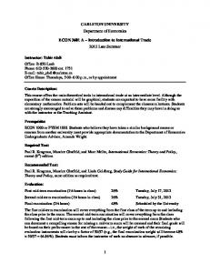
(a) A set I = {A01 (¯ a1 ), . . . , A0k (¯ ak )} of (ground) database atoms is a violation set for ic in instance D iff: (a1) A0j (¯ aj ) ∈ D, j = 1, . . . , k. (a2) There is a substitution θ : x¯ → U , such that {A1 (¯ x1 ), . . . , Am (¯ xm )}θ = I, and, for i = m + 1, . . . , m + s, Bi (¯ xi )θ is true in U. (b) The set of labeled violation sets of IC in D is I(D, IC) = {(I, ic) | ic ∈ IC and I is a violation set for ic}. 2 Here, A(¯ x0 )θ, with x¯0 ⊆ x¯, is the ground atom that results from applying θ to the variables in A(¯ x0 ); and {A1 (¯ x1 ), . . . , Am (¯ xm )}θ = {A1 (¯ x1 )θ, . . . , Am (¯ xm )θ}. In consequence, the substitution θ in the definition is a unifier of {A1 (¯ x1 ), . . . , Am (¯ xm )} and I. So, k ≤ m, and the predicates A0j must be among the Ai in (1). Notice that a violation set makes the conjunction in (1) true in D, and then ic becomes false in D. I(D, IC) contains the violation sets together with the constraint they violate, which is used as a label. In this way, the same set of tuples can be associated to different constraints. Elements (I, ic) of I(D, IC) will still be called violations sets. Notice that the definition of violation set can be applied to any extended denial. Example 13 (example 5 continued) A violation set for ic 1 is {t1 ,t4 } since, for θ(ID) = 1, θ(A) = 15, θ(C) = 25, θ(I) = CD and θ(P ) = 27, it holds {Buy(ID1 , I, P ), Client(ID, A, C)}θ = {t1 ,t4 }, and both (A < 18)θ and (P > 25)θ are true. Similarly, {t1 ,t5 } is also a violation set for ic 1 , and {t1 } and {t2 } are both violation sets for ic 2 . In consequence, I(D, IC) = {({t1 , t4 }, ic 1 ), ({t1 , t5 }, ic 1 ), ({t1 }, ic 2 ), ({t2 }, ic 2 )}. 2 Notice that the conflict hypergraph introduced in [12] for studying classic CQA wrt denial constraints has as vertices the database tuples in D; and as hyperedges, the violation sets for elements ic of IC. In our case, each hyperedge is labelled with its corresponding ic. If the denial constraints are functional dependencies, we obtain conflict graphs [3]. Example 14 (example 13 continued) The conflict hypergraph as shown in Fig. 1 contains four hyperedges, those corresponding to the violation sets ({t1 , t4 }, ic 1 ), ({t1 , t5 }, ic 1 ), ({t1 }, ic 2 ) and ({t2 }, ic 2 ). 2

ic2

t1

t2

ic 2

t3

ic 1

ic1 t4

t5

t6

Fig. 1. Conflict hypergraph

Definition 8 (a) Consider an instance D and a set IC of ICs. Let t be a tuple 22

in D such that t ∈ I ⊆ D, where (I, ic) is a violation set for ic ∈ IC in D. A database tuple t0 is a local repair of t (wrt I and ic) if: (a1) t0 uses the same database predicate as t. (a2) t0 has the same values as t in all the attributes but one fixable attribute. (a3) Replacing t by t0 solves the inconsistency wrt ic, i.e. ((I r {t}) ∪ {t0 }, ic) is not a violation set of IC in (D r {t}) ∪ {t0 }. (a4) There is no tuple t00 that simultaneously satisfies (a1)-(a3), differs from t on the same attribute as t0 , and ∆({t}, {t00 }) < ∆({t}, {t0 }), where ∆ denotes quadratic distance. (b) S(t, t0 ) = {(I, ic) | ic ∈ IC, t ∈ I and (I r {t}) ∪ {t0 } is not a violation set for ic in (D r {t}) ∪ {t0 }}. 2 A local repair t0 of t solves the violation of at least one IC where t participates, minimizes the distance from t, and differs from t in the value of only one attribute. Thus, if a tuple t is consistent, i.e. it does not belong to any violation set, then it has no local repairs. It holds S(t, t0 ) ⊆ I(D, IC), and the former set contains the violation sets that include t and are solved by replacing t0 by t. We will usually apply the notation S(t, t0 ) to a tuple t and one of its local repairs t0 . The attribute that has been changed by a local repair t0 of t is denoted by adiff (t, t0 ). 7 In the examples, we will usually write in bold the attribute values that are modified by local repairs. Example 15 (example 13 continued) Tuple t01 : Client(1, 15, 50) is a local repair of t1 , because: (a) It modifies only the value of the fixable attribute C in t1 ; (b) For ic 2 , replacing t1 by t01 solves the violation set ({t1 }, ic 2 ); and (c) There is no other tuple that solves the same violation set and is closer to t1 . In this case, adiff (t1 , t01 ) = C, and S(t1 , t01 ) = {({t1 }, ic 2 )}. Tuple t001 : Client(1, 18, 52) is also a local repair of t1 , with S(t1 , t001 ) = {({t1 , t4 }, ic 1 ), ({t1 , t5 }, ic 1 ), ({t1 }, ic 2 )}. Tuples t2 , t4 and t5 have one local repair each, namely t02 : Client(2, 16, 50), t04 : Buy(1, CD, 25), and t05 : Buy(1, DVD, 25), respectively, with S(t2 , t02 ) = {({t2 }, ic 2 )}), S(t4 , t04 ) = {({t1 , t4 }, ic 1 )}) and S(t5 , t05 ) = {({t1 , t5 }, ic 1 )}), respectively. The consistent tuple t3 has or needs no local repair. 2 5.2 Database repair problem as a set cover problem For a fixed sets IC of local denials, we can solve the instances of DROP (IC) by transforming them into instances of a Minimum Weighted Set Cover Optimization Problem (MWSCP). This problem is MAXSNP -hard [28,29], and its general approximation algorithms approximate within a logarithmic factor [28,14]. By concentrating on local denials, we will be able to generate versions 7

We recall that an attribute is associated to a unique database predicate and only one of its arguments.

23

of the MWSCP that can be approximated within a constant factor (cf. Section 5.3). Definition 9 For a database D and a set IC of local denials, the instance (U, S, w) for the MWSCP, where U is the underlying set, S is the collection of subsets of U , and w is the weight function,8 is given by: (a) U = I(D, IC); (b) S = {S(t, t0 ) | t0 is a local repair for a tuple t ∈ D}; and (c) w(S(t, t0 )) = ∆({t}, {t0 }). 2 By construction, all the S(t, t0 ) in the MWSCP are non empty. Also, since the ICs are local, the union of S is U . This holds since for each (I, ic) ∈ U , ic contains at least one fixable attribute A in a built-in, and there is tuple t ∈ I such that, by modifying t(A) we can get a local repair t0 of t such that I ∈ S(t, t0 ). Example 16 (example 5 and 15 continued) We illustrate this reduction from DROP to MWSCP , and give an idea about how we are going to use minimum set covers to obtain LS-repairs. Here, U = {({t1 , t4 }, ic 1 ), ({t1 , t5 }, ic 1 ), ({t1 }, ic 2 ), ({t2 }, ic 2 )}, and S = {S(t1 , t01 ), S(t1 , t001 ), S(t2 , t02 ), S(t4 , t04 ), S(t5 , t05 )}. The contents of each of the elements in S is shown in the table below. Elements of S are the columns, and their elements, the rows. An entry 1 means that the set of S contains the corresponding element in the first column; and a 0, otherwise. Set Weight ({t1 , t4 }, ic 1 ) ({t1 }, ic 2 ) ({t1 , t5 }, ic 1 ) ({t2 }, ic 2 )

S(t1 , t01 ) S(t1 , t001 ) S(t2 , t02 ) 4 9 1 0 1 0 1 1 0 0 1 0 0 0 1

S(t4 , t04 ) S(t5 , t05 ) 4 1 1 0 0 0 0 1 0 0

A minimum set cover for this problem is C1 = {S(t1 , t001 ), S(t2 , t02 )}, with total weight 10. It is a minimum cover, because the union of its elements is U , and there is no other cover with less weight. C1 shows that, by replacing t1 by t001 and t2 by t02 , all the violation sets are solved, i.e. they are no violation sets for the same constraint anymore. Actually, the database D0 obtained from D by replacing t1 by t001 and t2 by t02 is an LS-repair of D. These replacements lead to a consistent database for two reasons: (1) Since S(t1 , t001 ) and S(t2 , t02 ) together form a cover, all the inconsistencies are solved in D0 ; and (2) Since the constraints are local, no new inconsistencies are generated by these replacements. If the constraints were not local, the replacements would solve the initial inconsistencies, but might introduce new ones. Cf. Definition 11 and Lemma 5 below for a formal treatment of this idea. 8

In the corresponding MWSCP, we try to find (the weight of) a C ⊆ S, such that, for every u ∈ U , there is s ∈ C with u ∈ s (i.e. a set cover for U ), and C has minimum weight (given by the sum of the weights of its elements).

24

Another minimum cover, therefore also with weight 10, is C2 = {S(t1 , t01 ), S(t2 , t02 ), S(t4 , t04 ), S(t5 , t05 )}. The database D00 obtained from D by replacing t1 by t01 , t2 by t02 , t4 by t04 , and t5 by t05 is also an LS-repair. 2 As we can see, we could think of constructing an LS-repair by replacing each inconsistent tuple t ∈ D by a local repair t0 with S(t, t0 ) ∈ C, where C is a minimum set cover for the corresponding instance (U, S, w) of the MWSCP . The problem is that for a tuple t, it might be the case that S(t, t0 ) and S(t, t00 ) belong both to the minimum set cover C. In that case, it is not clear how to construct the LS-repair by replacing t. Example 17 Consider a schema with a predicate R(A, B, C, D), with KR = ¯ {A}, F(R) = {B, C}. The set IC of local denials contains ic 1: ∀¬(R(x, y, z, w), ¯ ¯ y > 3), ic 2 : ∀¬(R(x, y, z, w), y > 5, w > 7), and ic 3 : ∀¬(R(x, y, z, w), z < 4). The database instance D containing only the tuple t : R(1, 6, 1, 8) is inconsistent. Here, I(D, IC) = {({t}, ic 1 ), ({t}, ic 2 ), ({t}, ic 3 )}. There are three local fixes, namely, t1 : R(1, 3, 1, 8), t2 : R(1, 5, 1, 8) and t3 : R(1, 6, 4, 8). For them, S(t, t1 ) = {({t}, ic 1 ), ({t}, ic 2 )}, S(t, t2 ) = {({t}, ic 2 )} and S(t, t3 ) = {({t}, ic 3 )}. The instance of MWSCP is: Set Weight ({t}, ic 1 ) ({t}, ic 2 ) ({t}, ic 3 )

S(t, t1 ) S(t, t2 ) S(t, t3 ) 9 1 9 1 0 0 1 1 0 0 0 1

The only minimum cover is C = {S(t, t1 ), S(t, t3 )}. In this case, we could attempt to obtain an LS-repair by replacing t by both t1 and t3 , but this would result in a violation of the key constraint on R. However, the local repairs t1 and t3 can be combined into a new tuple t4 = R(1, 3, 4, 8), which is not a local repair, but solves all the inconsistencies. The database D0 obtained by replacing t by t4 is an LS-repair. 2 Our next results tells us that the replacement we made in the previous example is always possible. Lemma 4 Let C be a minimum cover for instance (U, S, w) of the MWSCP associated to D and IC. For different local repairs t0 , t00 of t such that S(t, t0 ), S(t, t00 ) ∈ C, it holds adiff (t, t0 ) 6= adiff (t, t00 ). Proof: Let us assume, by contradiction, that there are S(t, t0 ), S(t, t00 ) ∈ C such that adiff (t, t0 ) = adiff (t, t00 ) = A and t0 (A) < t00 (A). Since the ICs are local, either A is compared in all ICs in IC with either < or >. Without loss of generality, we assume the latter. Since t0 (A) < t00 (A), it is easy to see that S(t, t00 ) ⊆ S(t, t0 ). Thus, C r {S(t, t00 )} is also a cover. This implies that C is not minimum, and we have a contradiction. 2

25

This result may not hold if the cover is not minimum. This lemma allows us to combine in one tuple the local repairs that participate in a minimum cover. These combined tuple repairs will be used to construct a new consistent database. Definition 10 Let C be a minimum cover for instance (U, S, w) of the MWSCP associated to D, IC. (a) Let t1 , . . . , tn be the local repairs of t ∈ D, such that S(t, ti ) ∈ C, for i ∈ [1, n]. The combined local repair of t, denoted t? , is such that t? (A) = ti (A) when A = adiff (t, ti ), and t? (A) = t(A), otherwise. (b) If T ? = {(t, t? ) | there is t0 such that S(t, t0 ) ∈ C}, then we define D(C) = S ? ? 2 (t,t? )∈T [(D r {t}) ∪ {t }]. D(C) is the database instance obtained from D by replacing t by t? whenever (t, t? ) ∈ T ? . Notice that t? may not be a local repair of t, because it may change more that one attribute. However, t? is obtained from a set of tuples that modify only one attribute of t each. Whenever we have a cover C ⊆ S, where all the local repairs t0 in the elements S(t, t0 ) of C change different attributes values of t, we may compute the t? s, no matter if C is minimum or not. After that, T ? and its corresponding new instance D(C) can be computed as in Definition 10(b). Example 18 (example 17 continued) The combined local repair t? for t is obtained from the local repairs represented in C = {S(t, t1 ), S(t, t3 )}: t? becomes R(1, 3, 4, 8). Thus, T ? = {(t, R(1, 3, 4, 8))}, and D(C) = {R(1, 3, 4, 8)}, which is in fact the only LS-repair of D. 2 Now we can establish that there is a one-to-one correspondence between the minimum covers of the MWSCP and the LS-repairs. Theorem 5 If C is a minimum cover for instance (U, S, w) of the MWSCP associated to D, IC, then D(C) is an LS-repair of D wrt IC, and ∆(D, D(C)) = w(C). Furthermore, for every LS-repair D0 of D wrt IC, there exists a minimum cover C for the instance (U, S, w) of the M W SCP associated to D and IC, such that D0 = D(C). 2 In order to prove this theorem we need first some auxiliary concepts and technical lemmas. First, we will prove that local repairs do not introduce new inconsistencies when the denials are local. Definition 11 Consider an instance D and a set of local denials IC: (a) For (I, ic) a violation set for D and IC, define I[A r F] = {(R, t[A(R) r F(R)]) | there are R ∈ R and c¯ with t = R(¯ c) ∈ I}. (b) I(D, IC)[A r F] = {(I[A r F], ic) | (I, ic) ∈ I(D, IC)}. (c) Let t, t0 be database tuples such that {t} and {t0 } are rigid-comparable as instances, and t ∈ D. Replacing t by t0 in D does not generate new inconsistencies if I(D0 , IC)[A r F] r I(D, IC)[A r F] = ∅, where D0 = (D r {t}) ∪ {t0 }. 2

26

I[A r F] denotes the set of tuples of constants obtained from database tuples t in I by projecting the ts on their rigid attributes, and then annotating them with their predicate names R (to keep track of their origin). Example 19 (example 12 continued) In this case, IC = {ic 1 , ic 2 }, t is R(a, 1, 5), t0 is R(a, 1, 4), I(D, IC) = {({R(a, 1, 7)}, ic 1 ), ({R(a, 1, 7)}, ic 2 )}. For D0 = {R(a, 1, 4)}, I(D0 , IC) = {({R(a, 1, 4)}, ic 2 )}. To check if new inconsistencies are generated, we compute the difference between I(D0 , IC)[A r F] = {({(R, (a, 1))}, ic 2 )} and I(D, IC)[A r F] = {({(R, (a, 1))}, ic 1 ), ({(R, (a, 1))}, ic 2 )}. Since the difference is empty, replacing t by its local repair t0 does not generate new inconsistencies. 2 Lemma 5 If t0 is a local repair of a tuple t wrt instance D and a set of local denials IC, then replacing t by t0 in D does not generate new inconsistencies. 2 Proof: Let adiff (t, t0 ) = A. Since IC is local, attribute A can only appear in IC in -atoms, but not both. Without loss of generality, assume the latter is the case. So, t0 (A) < t(A). For D0 = (D r {t}) ∪ {t0 }, we need to prove that (I(D0 , IC )[A r F] r I(D, IC )[A r F]) = ∅. By contradiction, assume that for ic ∈ IC, there is a violation set (I 0 , ic) ∈ I(D0 , IC) such that there is no (I, ic) ∈ I(D, IC) with I[A r F] = I 0 [A r F]. Since the rigid values are kept in a repair, this is equivalent to saying that there is a violation set (I 0 , ic) ∈ I(D0 , IC) for which (m−1 (I 0 ), ic) 6∈ I(D0 , IC). Since t0 is the only difference between D and D0 , it holds t0 ∈ I 0 . But t0 (A) < t(A), the only difference between D and D0 is attribute A, and in all the constraints attribute A is compared only with >. Therefore, if (I 0 , ic) ∈ I(D0 , IC), then (m(I 0 ), ic) ∈ I(D, IC). We have a contradiction. 2 The following lemma justifies that an LS-repair can always be constructed from a set of local repairs that are combined as described in Definition 10. This lemma will allow us to prove later that, for every LS-repair D0 , there is minimum cover C such that D0 = D(C). Lemma 6 Consider an LS-repair D0 of D wrt IC, and L(D, D0 ) = {(t, t0 ) | t, t0 are R-tuples for some R ∈ R, t ∈ D, and there are an R-tuple t00 ∈ (D0 r D) and A ∈ A(R) such that t = m−1 (t00 ), t00 (A) 6= t(A), t0 (A) = t00 (A); and, for each B 6= A, t0 (B) = t(B)}. It holds: (a) For each (t, t0 ) ∈ L(D, D0 ), t0 is a local repair of t. (b) C(D, D0 ) = {S(t, t0 ) | (t, t0 ) ∈ L(D, D0 )} is a cover of the MWSCP associated to D and IC. (c) D(C(D, D0 )) = D0 . 2 For each tuple t ∈ D, the tuple m(t) in D0 (the t00 in the definition of L(D, D0 )) may differ in more than one attribute value from t. The set L(D, D0 ) contains the pairs (t, t0 ), such that t0 coincides with the modified version of t, i.e. m(t), in repair D0 in exactly one modified attribute value, but coincides with t at the

27

other attributes. That is, we are decomposing the modified versions of tuples in D into its “local repair components”. Thus, L(D, D0 ) traces back and finds the set of local repairs that can transform D into D0 . There will be as many local repairs of t in L(D, D0 ) as attribute values in t have been changed by m(t). If the local repairs obtained from L(D, D0 ) are combined as described in Definition 10, we would obtain a set T ? that is needed to transform D into D0 . For different local repairs t0 and t00 such that (t, t0 ), (t, t00 ) ∈ L(D, D0 ), it holds adiff (t, t0 ) 6= adiff (t, t00 ). Thus, it is possible to compute D(C(D, D0 )), even without proving that the cover C(D, D0 ) is minimum. However, later on we will show it actually is (cf. proof of Theorem 5). Example 20 (example 18 continued) The only LS-repair of D, that contains only tuple t : R(1, 6, 1, 8), wrt IC is D0 = {R(1, 3, 4, 8)}. This repair is obtained from D by two local repairs: one changing attribute B from 6 to 3 and another changing attribute C from 1 to 4. Thus, L(D, D0 ) = {(t, t0 ), (t, t00 )}, with t0 : R(1, 3, 1, 8) and t00 : R(1, 6, 4, 8). The repair D0 can be reconstructed from L(D, D0 ) by combining the local repairs as described in Definition 10. In fact, C(D, D0 ) = {S(t, t0 ), S(t, t00 )}, and T ? = {(t, t? )}, with t? = R(1, 3, 4, 8). Therefore, D(C(D, D0 )) = {R(1, 3, 4, 8)} = D0 . 2 Proof of Lemma 6: (a) Let (t, t0 ) ∈ L(D, D0 ). By the minimality of D0 as an LS-repair, the change of value in attribute A = adiff (t, t0 ) has to solve some inconsistency. More precisely, there are ic ∈ IC and I ⊆ D, such that (I, ic) is a violation set wrt D and IC, t ∈ I, and t0 solves the violation set, i.e. ((I r {t}) ∪ {t0 }, ic) is not a violation set wrt (D r {t}) ∪ {t0 }. We collect in a set all these violation sets. So, consider S = S(t, t0 ), the set of all the violation sets that are solved by replacing t by t0 . S is non empty, because (I, ic) ∈ S. Furthermore, t0 clearly satisfies conditions (a1)-(a3) for being a local repair of t through every (I, ic) in S. We have to check that (a4) holds for at least one element of S. Consider IC 0 = {ic ∈ IC | there is I with (I, ic) ∈ S}. Let us assume that attribute A appears in IC in comparisons of the type > (the case of comparisons with < is similar). Let c be the smallest constant with which A is compared through A > c in IC 0 . Let (I0 , ic 0 ) be an element of S such that A > c appears in ic 0 . Notice that for t to belong to the violation sets in S, it must hold t(A) > c. We have three cases: t0 (A) > c, t0 (A) < c, and t0 (A) = c. If t0 (A) > c, then (I0 , ic 0 ) cannot be solved by replacing t by t0 . Since (I0 , ic 0 ) ∈ S, we have a contradiction. If t0 (A) < c, we can construct the instance D00 = (D0 r {t0 }) ∪ {m(t)0 }, where m(t)0 coincides with m(t) (the modified version of t in D0 ) except at attribute A, for which m(t)0 (A) = c. The same inconsistencies will

28

be solved by D00 since c is the smallest value that appears in a comparison involving A. It holds ∆({D}, {D00 }) < ∆({D}, {D0 }); which contradicts the LS-minimality of D0 . Thus, it must be t0 (A) = c. In this case condition (a4) holds for (I0 , ic 0 ), because any tuple t00 with t00 (A) > c, i.e. closer to the original instance, will not solve the violation set (I0 , ic 0 ). In consequence, t0 is a local repair of t for (I0 , ic 0 ). (b) Now, we will prove that C(D, D0 ) = {S(t, t0 ) | (t, t0 ) ∈ L(D, D0 )} is a cover of the MWSCP. We have already proven that every S(t, t0 ) ∈ C(D, D0 ) is such that t0 is a local repair of t. Since D0 is an LS-repair of D wrt IC, the set of local repairs needed to construct it solve all the inconsistencies, and therefore C(D, D0 ) is a cover. 2 Proof of Theorem 5: We start proving the first statement, i.e. that the instance associated to a minimum cover is an LS-repair. Since the union of all the elements of a cover C is U , the local repairs represented by the cover solve all the violations sets in D. By Lemma 5, no new inconsistencies are added by applying the local repairs. Therefore, D(C) is a repair of D wrt IC. We need to prove that D(C) is an LS-repair. By contradiction, assume it is not. In this case, there exists an LS-repair D0 for which ∆(D, D0 ) < ∆(D, D(C)). Let C(D, D0 ) be the cover defined as in Lemma 6. It holds D(C(D, D0 )) = D0 . Also, for different local repairs t0 and t00 such that S(t, t0 ), S(t, t00 ) ∈ C(D, D0 ), we have adiff (t, t0 ) 6= adiff (t, t00 ). Since all the local repairs modify different values, w(C(D, D0 )) = ∆(D, D0 ). But ∆(D, D0 ) < ∆(D, D(C)) = w(C). Therefore, w(C(D, D0 )) < w(C). We obtain that C is not a minimum cover, and we have a contradiction. Now we prove the second statement, i.e. that for every LS-repair D0 there is a minimum cover C such that D(C) = D0 . Let C(D, D0 ) be defined as in Lemma 6. By Lemma 6, C(D, D0 ) is a cover of the MWSCP for D and IC. We need to prove that C(D, D0 ) is minimum. Let us assume, by contradiction, that there exists a minimum cover C 0 such that w(C 0 ) < w(C(D, D0 )). By the first claim in this theorem, D(C 0 ) is an LS-repair. Since C 0 is a minimum cover, by Lemma 4, no two local repairs of a tuple modify the same attribute. As a consequence, w(C 0 ) = ∆(D, D(C 0 )). By construction, C(D, D0 ) is such that no two local repairs of a tuple modify the same attribute. Thus, it holds that w(C(D, D0 )) = ∆(D, D(C)). This implies that ∆(D, D(C 0 )) < ∆(D, D(C(D, D0 ))) = ∆(D, D0 ), which contradicts the fact that D0 is an LS-repair. 2 Example 21 (example 16 continued) From the minimum cover C1 = {S(t1 , t001 ), S(t2 , t02 )}, we get t?1 = t001 = Client(1, 18, 52), and t?2 = t02 = Client(2, 16, 50), and therefore, D(C1 ) is instance D00 in Example 5. On the other hand, for the minimum cover C2 = {S(t1 , t01 ), S(t2 , t02 ), S(t4 , t04 ), S(t5 , t05 )}, the LS-repair D(C1 ) coincides with instance D0 in Example 5. 2

29

Proposition 5 The transformation of an instance of DROP (IC) into the instance of MWSCP , and the construction of database instance D(C) from a cover C for (U, S, w) can be done both in polynomial time in the size of D. Proof: It remains to verify that (U, S, w) can be computed in polynomial time in the size of D. Let n be the number of tuples in D. Notice that if mi is the number of database atoms in ic i ∈ IC, and m is the maximum value of the mi , there are at most nmi violation sets associated to ic i ∈ IC, each of them having between 1 and m tuples. Therefore, the size of U is O(nm × |IC|). The size of each S(t, t0 ) is bounded by the size of U . The size of S, i.e. the number of sets S(t, t0 ), is polynomially bounded by the size of D. In fact, there is one S(t, t0 ) for each local repair of t, and each tuple may have no more than |F| × |IC| local repairs, where F is the set of fixable attributes. Therefore, |S| is O(|F| × |IC| × |D|). The weight of each S(t, t0 ) is polynomially bounded by the maximum absolute value in an attribute in the database and the maximum absolute value of a constant appearing in IC (by an analysis similar to the one in Lemma 1). With respect to D(C), since C ⊆ S, C is polynomially bounded by the size of D. The generation of T ? and the replacements in D are easy. Therefore, the construction of D(C) can be done in polynomial time on |D|. 2 We have established that the transformation of DROP into MWSCP is an L-reduction [29]. If we apply this reduction to D and IC when IC is non-local, the instance D(C) for a cover C can still be constructed, as above. However, it may not satisfy IC, because repairing single inconsistent tuples through local repairs solves only the initial inconsistencies, but new inconsistencies can be introduced. This is the case in Example 6, which has a non-local set of denials.

5.3 Approximate LS-repairs via approximate minimum covers Now that we have transformed the database repair optimization problem into a weighted minimum set cover problem, we can apply approximation algorithms for the latter to approximate the former. Any cover C, even if not ˆ that is a repair of D. The better minimum, will generate a database D(C) the approximation, the closer will the repair be to an LS-repair. For example, using a greedy algorithm, MWSCP can be approximated within a factor log(N ), where N is the size of the underlying set U [14]. The approximation algorithm returns not only an approximation w ˆ to the optimal weight wo , but also a -not necessarily optimal- cover Cˆ for problem (U, S, w). As in Definition ˆ for D that may not be 10, the cover Cˆ can be used to generate a repair D(C) LS-minimum. 30

Example 22 (examples 5 and 21 continued) We show how to compute a solution to this particular instance of DROP using the greedy approximation algorithm for MWSCP presented in [14]. We start with Cˆ := ∅, S(ti , t0i )0 := S(ti , t0i ) for each S(ti , t0i ) ∈ S. Then, we add to C the set S(ti , t0i ) such that S(ti , t0i )0 has the maximum contribution ratio |S(ti , t0i )0 |/w(S(ti , t0i )0 ). In this case, the alternatives are: |S(t1 , t01 )|/w(S(t1 , t01 )) = 1/4, |S(t4 , t04 )|/w(S(t4 , t04 )) = 1/4, |S(t1 , t001 )|/w(S(t1 , t001 )) = 3/9, |S(t5 , t05 )|/w(S(t5 , t05 )) = 1. 0 0 |S(t2 , t2 )|/w(S(t2 , t2 )) = 1, The ratio is maximum for S(t2 , t02 ) and S(t5 , t05 ), so we can add any of them ˆ If we choose the first, we get Cˆ = {S(t2 , t02 )}. Now we compute the new to C. sets S(ti , t0i )1 := S(ti , t0i )0 r S(t2 , t02 )0 , and choose again an S(ti , t0i ) for Cˆ such ˆ that S(ti , t0i )1 maximizes the contribution ratio. Now S(t5 , t05 ) is added to C, 0 1 because S(t5 , t5 ) gives the maximum. We repeat this process until we get all the elements of U covered, i.e. all the sets S(ti , t0i )k become empty at some iteration point k. We finally obtain Cˆ = {S(t2 , t02 ), S(t5 , t05 ), S(t1 , t01 ), S(t4 , t04 )}. In this case, Cˆ is an optimal cover, ˆ is an LS-repair, namely D0 in Example 5. and therefore, D(C) 2 Since we are using a cover that is not necessarily minimum, Lemma 4 may not hold. This means that, for a tuple t, there might be two local repairs in the cover that modify the value of the same attribute; and t? cannot be computed as in Definition 10. This situation is shown in the following example. Example 23 (example 18 continued) The greedy algorithm in [14] returns the non-optimal cover Cˆ = {S(t, t1 ), S(t, t2 ), S(t, t3 )}. Here t1 = R(1, 3, 1, 8), t2 = R(1, 5, 1, 8) and t3 = R(1, 6, 4, 8) are all local repairs for the same tuple t, but now the first two of them modify its second attribute B. The tuples t1 and t2 solve different set of inconsistencies (violation sets); and those changes have to be made in order to solve them. Picking up randomly one of the two local repairs may leave the other set of inconsistencies unsolved. However, in this example, B always appears in the denial constraints in comparisons of the form B > c for a certain constant c.9 Furthermore, the values for the attributes other that B are the same in t1 and t2 . Therefore, we can construct the combined local repair by taking only the smallest value assigned to B in a local repair, namely 3 (the smallest constant c appearing in the comparisons B > c above). Thus, the combined local repair would be in this case t? = R(1, 3, 4, 8), which solves all the violation sets. 2 We need to modify Definition 10 to consider not only minimum covers, but any cover that might be returned by an approximation algorithm. 9

Recall that since the constraints are local, a fixable attribute is either used with < or > in IC but never both.

31

Definition 12 Let Cˆ be a (not necessarily minimum) cover for instance (U, S, w) of the MWSCP associated to D and IC. (a) For each tuple t ∈ D, and its local repairs t1 , . . . , tn for which S(t, ti ) ∈ C holds, the combined local repair t? is defined by the following conditions: (a1) t? [A] = ti [A] if there exists an i in [1, n] with A = adiff (t, ti ); and there is no other j in [1, n] with A = adiff (t, tj ) and tj [A] < ti [A] (tj [A] > ti [A]) if A is compared with > (resp. 7, w < 7), ¯ ¯ ic 2 : ∀¬(P (x, y, z), Q(x, w, v, u), y > 9, w < 6), ic 3 : ∀¬(P (x, y, z), y > 7, ¯ z > 2), and ic 4 : ∀¬(P (x, y, z), Q(u, w, v, x), y > 9, w > 2). D:

P

A a b

B 11 5

C 4 7

Q t1 t2

D a c

E 4 4

F 5 8

G f a

t3 t4

The violation sets are ({t1 , t3 }, ic 1 ), ({t1 , t3 }, ic 2 ), ({t1 }, ic 3 ) and ({t1 , t4 }, ic 4 ). The local repairs are: t01 : P (a, 7, 4), t001 : P (a, 9, 4), t03 : P (a, 7, 5, f ), t003 : P (a, 6, 5, f ), and t04 : P (c, 2, 8, a). The instance of the MWSCP is: Set Weight ({t1 , t3 }, ic 1 ), ({t1 , t3 }, ic 2 ), ({t1 }, ic 3 ) ({t1 , t4 }, ic 4 )

S(t1 , t01 ) S(t1 , t001 ) 16 4 1 0 1 1 1 0 1 0

S(t3 , t03 ) S(t3 , t003 ) S(t4 , t04 ) 9 4 4 1 0 0 1 0 0 0 1 0 0 1 1

The only minimum cover for this problem is C = {S(t1 , t01 )}, with weight 16. As expected, the associated repair D(C) also has distance 16 to D. However, a cover obtained by the greedy algorithm in [14] is Cˆ = {S(t1 , t001 ), S(t3 , t03 ), ˆ is: S(t3 , t003 ), S(t4 , t04 )}, with weight 21. The repair D(C)

32

P

A a b

B 9 5

C 4 7

Q t001 t2

D a c

E 7 2

F 5 8

G f a

t03 t04

This repair is not an LS-repair since the distance to D is 17 instead of 16. 2 Notice that, as illustrated in the previous example, for a cover C, it holds ∆(D, D(C)) ≤ w(C), with equality for a minimum cover. This is because, to obtain D(C), we may eliminate elements from C. Proposition 6 Given an instance D and a set IC of local ICs, the instance ˆ obtained from the cover Cˆ returned by the approximation algorithm, D(C), ˆ ≤ log(N ) × ∆(D, D0 ), where D0 is any is a repair. It also holds ∆(D, D(C)) LS-repair of D wrt IC, and N is the number of violation sets for D wrt IC. Proof: Since Cˆ is a cover, the local repairs that it represents solve all the violations sets in D. Since we are dealing with local ICs, the set of updates defined by T ? still solves all the inconsistencies. By Lemma 5, no new inconˆ is a repair sistencies are added by applying the local repairs. Therefore, D(C) of D wrt IC. ˆ ≤ log(N ) × ∆(D, D0 ). By definition of the We need to prove that ∆(D, D(C)) ˆ = Pt∈D ∆({t}, {t? }). Let {t1 , . . . , tn } be square distance, it holds ∆(D, D(C)) ˆ When comthe set of local repairs of t such that {S(t, t1 ), . . . , S(t, tn )} ⊆ C. ? puting t for t, some of the S(t, ti ) in Cˆ may not have been used. Assume that t∗ is built using the local repairs ti1 , . . . , tik , with {i1 , . . . , ik } ⊆ {1, . . . , n}. Thus, it holds ∆({t}, {t? }) = Σkj=1 ∆({t}, {tij }) ≤ Σni=1 ∆({t}, {ti }). In consequence, P ˆ ≤ Σ ∆({t}, {t? }) ≤ S(t,ti )∈Cˆ ∆({t}, {ti }). Finally, we obtain ∆(D, D(C)) P Pt∈D o ˆ ≤ log(N ) × w = log(N ) × S(t,ti )∈Cˆ w(S(t, ti )) = w S(t,ti )∈Cˆ ∆({t}, {ti }) = 0 0 ∆(D, D ), for every LS-repair D of D. 2 We have obtained that, for any set IC of local denials, there is a polynomial time approximation algorithm that solves DROP (IC) within an O(log(N )) factor, where N is the number of violation sets for D wrt IC. As mentioned before, this number N is polynomially bounded by |D| (cf. Proposition 5). N may be small if the number of inconsistencies or the number of database atoms in the ICs are small, which is likely the case in real applications. However, we can get an even better approximation via a cover Cˆ obtained with an approximation algorithm for a special case of the MWSCP : When the number of occurrences of an element of U in elements of S (its frequency) is bounded by a constant. For this case of the MWSCP there are approximations based on “linear relaxation” that provide a constant approximation factor [23, Chapter 3]. This is clearly the case in our application, being m × |F| × |IC | a constant bound (independent from |D|) on the frequency of each element of U , where m is the maximum number of database atoms in an IC. Theorem 6 There is a polynomial time approximation algorithm that, for a 33

ˆ of D wrt given instance D and a set IC of local ICs, returns a repair D(C) 0 ˆ IC, such that ∆(D, D(C)) ≤ c × ∆(D, D ), where c is a constant and D0 is any LS-repair of D. 2

6

One Atom Denials and Conjunctive Queries

In this section we concentrate on the common case of one database atom denials (1AD), i.e. of the form ∀¬(A, B), where atom A has a predicate in R, and B is a conjunction of built-in atoms. One atom denials are used in practice. For example, they capture range constraints. They can also be used as constraints on census data, which is usually represented as a single relation [18]. It is not difficult to produce examples of instances that have exponentially many LS-repairs wrt 1ADs. Thus, CQA is not necessarily easier under 1ADs. Actually, we will see below that some decision problems around CQA are NP -hard. For 1ADs, we can identify tractable cases for CQA under LS-repairs by reduction to CQA for (tuple and set-theoretic) repairs of the form introduced in [2] for key constraints. This is because each violation set (cf. Definition 7) contains one tuple, maybe with several local repairs, but all sharing the same rigid values. So, now the problem consists in choosing one from different tuples with the same rigid values (cf. proof of Theorem 7 below). The transformation preserves consistent answers to both ground and open queries. The “classic” -tuple and set oriented- CQA problem as introduced in [2] has been studied in detail for key dependencies in [12,19]. In particular, for tractability of CQA in our setting, we can use results and algorithms obtained in [19] for the classic framework. The join graph G(Q) [19] of a conjunctive query without built-ins Q is a directed graph whose vertices are the database atoms in Q. There is an edge from L to L0 if L 6= L0 and there is a variable w that occurs at the position of a non-key attribute in L and also occurs in L0 . Furthermore, there is a self-loop at L if there is a variable that occurs at the position of a non key attribute in L, and at least twice in L. For a conjunctive query without repeated database predicates and without built-ins Q, we write Q ∈ CForest if G(Q) is a forest and every non-key to key join of Q is full i.e. involves the whole key. Classic CQA wrt key constraints is tractable for queries in CForest [19]. Theorem 7 For every fixed set of 1ADs and query in CForest , consistent query answering under LS-repairs is in PTIME . 34

Proof: Based on the tractability results in [19], it suffices to show that the LSrepairs for a database D are in one-to-one and polynomial time correspondence with the classic repairs based on tuple deletions [2,12] for a database D0 wrt a set of key dependencies. Since we have 1ADs, the violation sets will have a single element. Thus, for an inconsistent tuple t wrt a constraint ic ∈ IC, it holds ({t}, ic) ∈ I(D, IC ). Since all the violation sets are independent, in order to compute an LS-repair for D, we have to generate independently all the local repairs t0 for all inconsistent tuples t such that there exists and ic ∈ IC with ({t}, ic) ∈ I(D, IC ). Those local repairs can be found by considering all the candidate repairs (not necessarily LS-minimum) that can be obtained by replacing, in each tuple, the flexible attributes that appear in the ICs by all the values in the intervals around the borders and around the values in D (cf. Lemma 1). Then, one can check which of candidate repairs satisfy IC. Finally, those that minimize ∆({t}, {t0 }) are chosen. The number of repair candidates per tuple in the database is O((|D| × |A|2 + |Borders(IC)| × |A|)|F | ), where A is the set of attributes and F is the set of fixable attributes. Thus, the total number of repair candidates is O(|D|(|D| × |A|2 + |Borders(IC)| × |A|)|F | ), which is polynomial in the size of D. Let us now define a database D0 consisting of the consistent tuples in D, together with all the local repairs of the inconsistent tuples. By construction, D and D0 share the same rigid values. Since each inconsistent tuple in D may have more than one local repair, D0 may become inconsistent wrt its key constraints. Each classic repair of D0 , i.e. obtained by tuple deletions, will choose one local repair from D0 for each inconsistent tuple t of D, and therefore will determine an LS-repair of D wrt IC. Conversely, every LS-repair can be obtained in this way. 2 For queries Q returning numerical values only, e.g. scalar aggregate queries, which is common in our framework, it is natural to use a range semantics for CQA [3]. In this case, the consistent answer to Q is the pair consisting of the max-min and min-max answers, i.e. the infimum and supremum, resp., of the set of answers to Q obtained from LS-repairs. In other words, the consistent answer to a numerical query Q is the shortest interval [max-min,min-max], such that for every LS-repair D0 , Q(D0 ) ∈ [max-min,min-max]. We can see that the max-min and min-max answers to a query are the minimum and the maximum answers, resp., considering all LS-repairs. So, finding these values becomes a minimization and a maximization problem, resp., over the class of LS-repairs. Correspondingly, the decision problems of CQA under the range semantics consist in determining if a numerical query Q has its answer: (a) ≤ k1 in some LS-repair (the max-min case); or (b) ≥ k2 for some LS-repair (the min-max case).

35

Our next result exhibits, for each of the common aggregate functions, a set of denials and a scalar aggregate conjunctive query for which at least one of these two decision problems of CQA becomes NP -complete. Theorem 8 For each of the aggregation functions sum, count, count distinct, and average, there is a fixed set of 1ADs and a fixed aggregate acyclic conjunctive query with one occurrence of the function, such that CQA under the range semantics is NP -complete. 2 For the proof of this theorem we need a preliminary result. Lemma 7 Consider a regular undirected graph G = (V, E) of degree 3 (i.e. all the vertices have degree 3), and a function F from sets of vertices S to nonnegative integers defined as follows: l 3 (1) For S ⊆ V, and ( v ∈ V, F (S, v) := |T (S, v)| , where: 0 0 0 {v | v ∈ (V r S) and {v, v } ∈ E} , v ∈ S T (S, v) := ∅ , v 6∈ S P l (2) F (S) := v∈S F (S, v). The maximum value of F (S) over all possible sets S ⊆ V is (33 × |I|), for I a maximal (wrt set inclusion) independent set. 2 Proof: Let us first assume that S is an independent set, not necessarily maximal. In this case the value F (S) is 33 × |S|, because each element v ∈ S is connected to three vertices in V r S. Then, among independent sets, the maximum value for F (S) is 33 × m, where m is the maximum cardinality of an independent set. For S ⊆ V, let G[S] denote the subgraph (S, ES ), where ES are all the edges {v, v 0 } ∈ E such that v, v 0 ∈ S. Now, if S is not an independent set, there exists a maximum independent set IS of G[S]. Every v ∈ (V r S) is adjacent to at least one vertex in IS , otherwise IS ∪ {v} would be an independent set contained in S which is a proper extension of IS , contradicting our choice of P IS . Now, define Fext (S, v) = (F l (S, v) + {v,v0 }∈E F l (S, v 0 )). Since every edge v 0 ∈ (S r IS ) is adjacent to IS , it is easy to see that: F (S) ≤

X

Fext (S, v).

(2)

v∈I

We want to prove that F (S) ≤ F (IS ). This, combined with equation (2), P shows that it suffices to prove that v∈IS Fext (S, v) ≤ F (IS ). Since F (IS ) = P P P l l v∈IS F (IS , v), we need to prove that v∈IS Fext (S, v) ≤ v∈IS F (IS , v). It l is sufficient to prove that Fext (S, v) ≤ F (IS , v) is true for every v ∈ IS . For v ∈ IS and S 0 = (S r IS ), we have the following cases: (1) If v is adjacent to one vertex in S 0 , then Fext (S, v) ≤ 23 + 23 , and F l (IS , v) = 33 . In consequence, Fext (S, v) ≤ (F l (IS , v) − 11). (2) If v is adjacent to two vertices in S 0 , analogously to (1), we get Fext (S, v) ≤ 36

(F l (IS , v) − 10). (3) If v is adjacent to three vertices in S 0 , analogously to (1), we get Fext (S, v) ≤ (F l (IS , v) − 3). Thus, we have proved that Fext (S, v) ≤ F l (IS , v), and therefore, that F (S) ≤ F (IS ). We also know that, since IS is an independent set, that F (S) ≤ F (IS ) ≤ 33 × m. 2 Proof of Theorem 8: In all the cases, membership to NP is a consequence of the existence of a polynomially bounded and polynomial-time verifiable certificate, as established in Theorem 1. Now we consider hardness. (a) For sum: By reduction from the NP -hard problem Independent Set for Cubic Planar Graphs [21], where the vertices of the graph have all degree 3. Given an undirected graph G = (V, E) of degree 3, and a lower bound k for the size for a maximum independent set, we create a predicate Ver (V, C1 , C2 ), where the key V takes vertices as values, and C1 , C2 are fixable and may take values 0 or 1, but are all equal to 0 in the initial instance D. This relation is subject to the denial ic : ∀v, c1 , c2 ¬(Ver (v, c1 , c2 ), c1 < 1, c2 < 1). D is inconsistent wrt this constraint, and, in any of its LS-repairs, each vertex v will have associated a tuple Ver (v, 1, 0) or Ver (v, 0, 1), but not both. Each LS-repair D0 of the database defines a partition of V into two subsets: S, with those v with Ver (v, 1, 0) ∈ D0 ; and S 0 , with those v with Ver (v, 0, 1) ∈ D0 . Clearly S ∪ S 0 = V and S ∩ S 0 = ∅. We also use predicate Edge(V1 , V2 , W ), with rigid attributes only, whose extension contains Edge(v1 , v2 , 1) and Edge(v2 , v1 , 1) for {v1 , v2 } ∈ E. So, every vertex v appears exactly 3 times in each argument of Edge-tuples in D. Consider the ground aggregate conjunctive query Q: q(sum(w0 )) ← Ver (v1 , c11 , c12 ), c11 = 1, Edge(v1 , v2 , w0 ), Ver (v2 , c21 , c22 ), c21 = 0, Edge(v1 , v3 , w1 ), Ver (v3 , c31 , c32 ), c31 = 0, Edge(v1 , v4 , w2 ), Ver (v4 , c41 , c42 ), c41 = 0. Given an LS-repair as a partition of a set of vertices into two subsets S and S 0 , for each vertex v ∈ S, the body of Q will be satisfied m3 times, where m is the number of vertices of S 0 that are adjacent to elements in S. This happens because the query has three pairs of predicates Edge, Ver , each predicate can be satisfied m times, and they are independent from each other (there are no equality, non-equality or predicates connecting them). In consequence, the whole body of the query will be satisfied m3 times. Each satisfying assignment of the body of the query brings value 1 to the multiset (w0 ) which is under the sum aggregation function. That is, query Q computes the nonnegative integer function F , such that F (S) gives the sum of cubes of the number of vertices of V r S that are adjacent to vertices in S. More precisely, F (S) = Q(D0 ), for D0 ∈ Rep(D, IC ) and S = {v | Ver (v, 1, 0) ∈ D0 }.

37

Since this function is nonnegative and its value is zero for S = ∅ and S = V, we have that its minimum value in the repairs is zero. We are interested in the maximum value for Q in Rep(D, IC ), i.e. the min-max answer introduced in [3]. From Lemma 7, we have that the answer to query Q is at most 33 × |I|, with I a maximum independent set. In consequence, the min-max answer for Q is 33 × m, with m the cardinality of the maximum independent set. Thus, there is an independent set of size at least k iff min-max answer to Q ≥ 33 × k. (b) For count: Basically the same proof as for (a) applies. Only the query has to be changed to: q(count) ← Ver (v1 , c11 , c12 ), c11 = 1, Edge(v1 , v2 , w0 ), Ver (v2 , c21 , c22 ), c21 = 0, Edge(v1 , v3 , w1 ), Ver (v3 , c31 , c32 ), c31 = 0, Edge(v1 , v4 , w2 ), Ver (v4 , c41 , c42 ), c41 = 0, w0 = 1. (c) For count distinct: By reduction from MAXSAT. Assume that an instance for MAXSAT is given. It consists of a set P of propositional variables, a collection C of clauses over P, and a positive integer k. The question is whether at least k clauses can be satisfied simultaneously. The answer will be Yes exactly when a question of the form countd ≤ (k − 1), with countd defined by an aggregate query over a database instance (both of them to be constructed below), gets answer No under the min-max semantics. Define a predicate Var (U, V1 , V2 ), being the first attribute the key, and the second and third are fixable (the denial below and the minimality condition will make them take values 0 or 1). The initial database contains Var (u, 0, 0) for every u ∈ P. Another predicate, Clause(u, c, s), has no fixable attributes. Its extension contains Clause(u, c, s) for every occurrence of variable u ∈ P in a clause c ∈ C, where s an assignment for u satisfying clause c. The IC is ∀u, v1 , v2 ¬(Var (u, v1 , v2 ), v1 < 1, v2 < 1). The acyclic query is q(countd (c)) ← Var (u, v1 , v2 ), Clause(u, c, s), v1 = s, where countd denotes the “count distinct” aggregation function. Its answer tells us how many clauses are satisfied in a given LS-repair. The max value taken on a LS-repair, i.e. the min-max answer, will be the maximum number of clauses which may be satisfied for MAXSAT. (d) For average: By reduction from 3-SAT. We use the same predicate Var (U, V1 , V2 ) and IC as in (c). Now, we encode clauses as tuples in the extension of a predicate Clause(Val , Var1 , Val1 , Var2 , Val2 , Var3 , Val3 ), which has no fixable attributes. The extension contains tuples Clause(val, var1 , val1 , var2 , val2 , var3 ), where var1 , var2 , var3 are the propositional variables in the clause (in any order), val1 , val2 , val3 are all the possible combinations of truth assignments to variables (at most eight combinations per clause); and val is the corresponding truth value taken by the clause (0 or 1) given the values val i . Now, the acyclic query q(avg(v )) ← Clause(v, u1 , v1 , u2 , v2 , u3 , v3 ), Var (u1 , v1 , v10 ), Var (u2 , v2 , v20 ), 38

Var (u3 , v3 , v30 ) takes a maximum value 1 in an LS-repair, i.e. the min-max answer to q is 1, iff the formula is satisfiable. 2 Notice that for the four aggregation functions one 1AD suffices (plus the 1ADs that force numerical values not to be less that 0). For sum and count we use a reduction from the Independent Set Problem with bounded degree 3 [21]. The general Independent Set Problem has bad approximation properties [23, Chapter 10]. The Bounded Degree Independent Set has efficient approximations within a constant factor that depends on the degree [22]. Theorem 9 For any set of 1ADs and conjunctive query with sum over a non negative attribute, there is a polynomial time approximation algorithm with constant factor for determining the min-max answer for CQA. 2 The factor in this theorem depends upon the ICs and the query, but not on the size of the database. The acyclicity of the query is not required. The algorithm is based on a reduction of our problem to satisfying a subsystem with maximum weight of a system of weighted algebraic equations over the Galois field with two elements GF [2] (a generalization of problems in [20,33]). For the latter problem, a polynomial time approximation similar to the one for MAXSAT can be given [33]. The long proof of this theorem is given in Appendix A in [6].

7

Extensions

7.1 Dependencies between attributes The notion of LS-repair that we introduced can be seen as a first approach to the problem of defining and computing a semantically correct data set that is close to the one at hand. Thinking of census like applications, the idea that key constraints are satisfied makes sense. Data forms usually come partially filled out, with the data for the identification fields already entered. It is the data that is entered in situ the one that is subject to errors. Considering the possible violation of the key constraints in this picture would require much more research. Our results rely on the hardness of the key constraints. We are also making the reasonable assumption that the dependencies between fixable attributes are captured by the denial constraints, but the errors that one can make when entering the individual attribute values are independent from each other. A more sophisticated model could consider some sort of stochastic dependency between the errors made in groups of attribute values. This dependency should be captured by the distance function. This is an interesting venue to explore that has to be left for future research. 39

7.2 Minimum distribution-variation repairs Repairing a database under minimization of the square distance to the original database may not preserve the statistical or aggregate properties of the original data, which in some applications could be relevant, like in census data. Given that there may be several LS-repairs, we may prefer those that preserve the data distribution. As a first step in this direction, one could choose those LS-repairs such that, for each fixable attribute, the frequency of values in the repair stay as close as possible to the frequency of values in the original database. This is one way of capturing the preservation of the data distribution. This choice assumes that the different attributes are stochastically independent. Without attempting to develop this direction in full, we briefly investigate in the following a first possible approach. A deeper analysis of this class of LS-repairs under the independence assumption, and also the study of preservation of statistical properties when attributes are stochastically correlated are both material for future research. Definition 13 Let D and D 0 be instances over the schema Σ = (U, R, B, A), and R ∈ R. (a) The distribution distance between D and D 0 wrt attribute P 0 2 0 A of R is ∆R.A a∈Dom(A) (count(a, R.A, D) − count(a, R.A, D )) , d (D, D ) = where count(a, R.A, D) gives the number of occurrences of value a in A of R in instance D. (b) The distribution distance ∆d (D, D0 ) between D and D 0 is the maximum of the distribution distances over all relations and their attributes. (c) Given set of ICs IC, D0 is a minimum distribution variation repair (MDVrepair) of D wrt IC if D0 is an LS-repair that also minimizes ∆d (D, D 0 ). 2 Example 26 Consider the IC ∀N, E, S¬(Emp(N, E, S), E < 5, S > 5), which requires that no employee with experience shorter than 5 years gets a salary higher than 5 thousand. The inconsistent instance D = {Emp(Ann, 4, 6), Emp(Bill, 3, 7), Emp(Chris, 2, 2), Emp(Dan, 6, 6)} has the following LS-repairs: D1 = {Emp(Ann, 4, 5), Emp(Bill, 3, 5), Emp(Chris, 2, 2), Emp( Dan, 6, 6)}, D2 = {Emp(Ann, 4, 5), Emp(Bill, 5, 7), Emp(Chris, 2, 2), Emp(Dan, 6, 6)}, D3 = {Emp(Ann, 5, 6), Emp(Bill, 3, 5), Emp(Chris, 2, 2), Emp(Dan, 6, 6)}, D4 = {Emp(Ann, 5, 6), Emp(Bill, 5, 7), Emp(Chris, 2, 2), Emp(Dan, 6, 6)}. The distance is ∆(D, Di ) = 12 + 22 = 5 for i = 1, 2, 3, 4. N S E ∆d (D, D1 ) = M ax{∆N d (D, D1 ), ∆d (D, D1 ), ∆d (D, D1 )}, with ∆d (D, D1 ) = S E 0, ∆d (D, D1 ) = 0, and ∆d (D, D1 ) = (count(5, S, D) − count(5, S, D1 ))2 + (count(6, S, D)− count(6, S, D1 ))2 + (count(7, S, D) − count(7, S, D1 ))2 = 22 + 12 + 12 = 6. Thus, ∆d (D, D1 ) = 6. N S E ∆d (D, D2 ) = M ax{∆N d (D, D2 ), ∆d (D, D2 ), ∆d (D, D2 )}, with ∆d (D, D1 ) =

40

2 0, ∆E d (D, D2 ) = (count(3, S, D) − count(3, S, D2 )) + (count(5, S, D)− count(5, S, D2 ))2 = 12 +12 , and ∆Sd (D, D2 ) = (count(5, S)− count(5, S, D2 ))2 + (count(6, S, D) − count(6, S, D2 ))2 = 12 + 12 . Thus, ∆d (D, D2 ) = 2.

This shows that repair D1 has a bigger impact over the distribution than D2 . Then, if we want to keep the statistical properties of the database we will prefer D2 better than D1 . Analogously, we can obtain ∆d (D, D3 ) = 2 and ∆d (D, D4 ) = 6. Then, ∆d (D, D2 ) = ∆d (D, D3 ) < ∆d (D, D1 ) = ∆d (D, D4 ), and the MDV-repairs are D2 and D3 . 2 From Theorem 2 and the fact that for a database there is an LS-repair if and only if there is a MDV-repair, we obtain Proposition 7 The problem of existence of MDV-repairs under linear constraints is NP -complete. 2 7.3 Aggregation Constraints We may consider aggregation constraints (ACs) [31] expressed in terms of aggregation functions, like sum, count, average. It is natural and common to use those functions when processing numerical data. Filtering ACs impose conditions on the tuples over which aggregation is applied, e.g. sum(A1 : A2 = 3) > 5 contains a sum over A1 of tuples with A2 = 3, and checks if this sum is greater that 5. Multi-attribute ACs allow for arithmetical combinations of attributes as arguments for sum, e.g. sum(A1 + A2 ) > 5 and sum(A1 × A2 ) > 100. If an AC has attributes from more than one predicate, it is multi-relation, e.g. sumR1 (A1 ) = sumR2 (A1 ), otherwise it is single-relation. Having aggregation constrains together with denial constrains has an impact on the class of possible repairs. For example, consider the relational predicate R(A, B), with key A and fixable attribute B. If we have IC = {∀x, y¬(R(x, y), y > 1), sum(B) = 10}, any database with less than 10 tuples has no repairs. It is not difficult to see that for a fixed set IC of ICs containing denials and aggregation constraints, NE (IC) is decidable. Here we will investigate the decision NE = {(D, IC) | Rep(D, IC) 6= ∅}, of existence of LS-repairs, whose instances in this case consist both of a database instance and a set of constraints (and a corresponding schema). We consider the variant of CQA where ICs are also part of the instances. Theorem 10 Under extended linear denials and complex, filtering, multiattribute, single-relation, aggregation constraints, the problems NE of existence of LS-repairs, and CQA under the skeptical semantics are undecidable. Proof: (sketch) Hilbert’s 10th problem on existence of integer solutions to 41

diophantine equations can be reduced to NE . More precisely, given a diophantine equation, it is possible to construct a database D and a set of ICs IC such that the existence of an LS-repair for D wrt IC implies the existence of a solution to the equation, and viceversa. An example can be found in Appendix B in [6]. For CQA, apply Proposition 2. A more detailed sketch of the proof for NE and a representative example is given in Appendix B. in [6]. 2 7.4 Other distances Our results for the square distance rely basically on the additivity of the distance on the tuples of the database and its monotonicity on the absolute values of the differences between values for the same attribute. The property of polynomial-time computability of the distance function is also required. Any distance that satisfies these properties can be used instead of the L2 distance, obtaining the same complexity results. In particular, all the results apply to the “city” distance (or L1 distance) given by the sum of those absolute differences. Of course, when using the L1 distance, we may get a different set of repairs for the same database. The approximation algorithm can also be used by computing the weights using the L1 instead of the L2 distance. Thus, the general complexity and approximability results still hold. For example, the optimization and implementation of the approximation in [27] of the algorithm for the DROP problem presented here uses the L1 distance, without any essential changes wrt the treatment based on the L2 distance. The edit distance (ED) between two strings is the minimum number of substitutions, deletions and insertions of characters that are needed to transform one string into the other. The hamming distance between two strings of the same length is the number of positions that have different characters. The hamming distance is an upper bound for the edit distance. For example, HD(234, 345) = 3, but ED(234, 345) = 2. These distances are used in data editing, but they are more appropriate for strings of characters, and not for numerical data. Actually, our results would not apply to the edit distance or the hamming distance, because they do not monotonically increase over the absolute value of the difference between two attributes. For example, for the numbers 21, 30 and 31, ED(21, 30) = 2 > ED(21, 31) = 1. However, since |21 − 31| > |21 − 30|, the edit distance does not monotonically increase over the absolute value of the difference. The same example can be used for the hamming distance, because HD(21, 30) = ED(21, 30) and HD(21, 31) = ED(21, 31). Another problem with the edit and hamming distance is that there are too many possible repairs to consider. For example, the database D = {P (a, 150)}, where the first attribute is the primary key and the second attribute is fixable, is inconsistent wrt P (x, y) → y ≥ 200. There exists only one LS-repair (under the quadratic distance): D0 = {P (a, 200)}. If instead, we consider the edit 42

distance, there are more than 40 repairs at distance one. For example: D1 = {P (a, 250)}, D2 = {P (a, 350)}, D3 = {P (a, 1050)}, D4 = {P (a, 1530)}, D5 = {P (a, 1590)}, D6 = {P (a, 6150)}, D7 = {P (a, 1507)}, etc.

8

Conclusions

We have shown that fixing numerical values in databases poses many new computational challenges that had not been addressed before in the context of consistent query answering. These problems are particularly relevant in census like applications, where the problem of statistical data editing [9,32] is a common and difficult task. Also our concentration on aggregate queries is particularly relevant for this kind of statistical applications. In this paper we have just started to investigate some of the many problems that appear in this context, and several possible extensions deserve to be explored. We concentrated on integer numerical values, which provide a useful and challenging domain. Considering real numbers in fixable attributes opens many new issues, requires different approaches; and must be left as a subject of future research. Some of the results presented here carry over to the case of real numbers. However, apart from the technical problems, the main complication is to come up with a right repair semantics in the presence of real numbers, in particular in comparisons of attributes. For example, if two attributes A, B take the same value, but a constraint prevents this from happening, it is not clear what new values have to be given to them in order to restore consistency. Most likely making them differ by an infinitesimal quantity would not make much sense in most of the applications. We could accept an epsilon of error in the distance, in such a way that if, for example, the distance of a repair is 5 and the distance to another repair is 5.001, we could take both of them as (minimum) LS-repairs. What is essential about the numerical domain, in our case, the integers, is that we have a discrete linear order and a numerical distance function that is monotonic on the length of the interval between two arbitrary elements. In consequence, the framework established in this paper could be applied to qualitative attributes which have an implicit linear order given by the application. Also numerical distances, like the ones introduced here, could be applied to domains other than numerical if their elements can be naturally mapped to numbers. The result we have presented for fixable attributes that are all equally relevant (αA = 1 in Definitions 1 and 2) should carry over without much difficulty to the general case of arbitrary weighted repairs. We have shown how to extend our approach in order to consider minimum distribution variation LS-repairs that keep, in some sense, the overall statistical properties of the database. 43

Other open problems refer to the identification of cases of polynomial complexity for linear denials with more that one database atom; approximation algorithms for the DROP for non-local cases; and approximations to CQA for other aggregate queries. More research on the impact of aggregation constraints on LS-repairs is needed. For related work, we refer mainly to the literature on consistent query answering. In [4] an earlier survey with abundant references can be found. More recent surveys can be found in [5,13]. Most of the research on consistent query answering has been carried out appealing to a tuple oriented repair semantics, i.e. minimal repairs are obtained through tuple insertions or deletions. Under the set-theoretic, tuple-based semantics, [12,11,19] present results on complexity of CQA for conjunctive queries, functional dependencies and foreign key constraints. A majority semantics was studied in [26] for database merging. The range semantics for CQA of aggregate queries was introduced and investigated in [3]. In that paper, the NP -completeness of CQA for atomic aggregate queries, tuple-based and set-oriented repairs, and functional dependencies was established. Previous research reported in [34] and [18] is the closest to our work, because changes in attribute values are basic repair actions. However, the peculiarities of numerical values and quantitative distances between databases are not investigated. Recent research presented in [17] investigates the complexity of repair checking and CQA wrt aggregation constraints. In this case, the constraints impose linear restrictions on summarizations. The repair semantics is based on changes of numerical attribute values, as in our case. However, the distance between instances does not consider the numerical values, but the set of changes wrt cardinality or set inclusion. Queries are atomic, without aggregation. Computational mechanisms are not considered. However, in [16] the authors present a system that uses linear programming techniques for computing a repair wrt aggregation constraints. The repair minimizes the number of changes of attribute values. In [27], optimizations, the implementation, and experiments of/with the approximation algorithm for DROP are presented. A repair semantic based on changes of attribute values is also considered in [7]. The ICs considered are functional and inclusion dependencies. Database tuples have numerical weights that may reflect provenance in data integration. In consequence, a repair has a weight that reflects the weights of the tuples modified by it. Except for these external weights, numerical attributes values are not investigated. The authors concentrate of developing and investigating heuristics for computing minimum cost repairs, but consistent query answering is not addressed.

44

There is interesting work in the area of statistical data editing [32]. Similar to integrity constraints, edits are used to express conditions that a data set should satisfy [15]. Edits can be expressed as linear inequalities. There are several alternative ways of modifying the data so that edits are satisfied [15,10,8,9]. Those methods are tailored to finding a single “repair”. Consistent query answering has not been considered in that area, and, to the best of our knowledge, the complexity of the problem has not been investigated. Acknowledgments: Research supported by NSERC, CITO/IBM-CAS Student Internship Program, and EU projects: Sewasie, Knowledge Web, and Interop. L. Bertossi is Faculty Fellow of IBM Center for Advanced Studies (Toronto Lab.). Part of this work was done while L. Bravo was doing her PhD at Carleton University. A. Lopatenko was working at the Free University of Bozen-Bolzano and studying at the University of the Manchester while doing this research. Extremely valuable feedback from anonymous referees is much appreciated.

References [1] Abiteboul, S., Hull, R. and Vianu, V. Wesley, 1995.

Foundations of Databases. Addison-

[2] Arenas, M, Bertossi, L. and Chomicki, J. Consistent Query Answers in Inconsistent Databases. In Proc. ACM Symposium on Principles of Database Systems (PODS 99), 1999, pp. 68-79. [3] Arenas, M, Bertossi, L. and Chomicki, J., He, X., Raghavan, V., and Spinrad, J. Scalar Aggregation in Inconsistent Databases. Theoretical Computer Science, 2003, 296:405–434. [4] Bertossi, L. and Chomicki, J. Query Answering in Inconsistent Databases. In Logics for Emerging Applications of Databases, J. Chomicki, G. Saake and R. van der Meyden (eds.), Springer, 2003. [5] Bertossi, L. Consistent Query Answering in Databases. ACM Sigmod Record, June 2006, 35(2):68-76. [6] Bertossi, L., Bravo, L., Franconi, E. and Lopatenko, A. The Complexity and Approximation of Fixing Numerical Attributes in Databases Under Integrity Constraints. Extended version with appendices. http://www.scs.carleton.ca/∼ bertossi/papers/longIS07.pdf [7] Bohannon, P., Fan, W., Flaster, M. and Rastogi, R. A Cost-Based Model and Effective Heuristic for Repairing Constraints by Value Modification. In Proc. ACM International Conference on Management of Data (SIGMOD 05), 2005, pp. 143-154.

45

[8] Boskovitz, A., Gor´e, R. and Hegland, M. A Logical Formalisation of the FellegiHolt Method of Data Cleaning, Springer LNCS 2810, 2003, pp. 554-565. [9] Boskovitz, A., Gor´e, R. and Wong, P. Data Editing and Logic. Proc. Work Session on Statistical Data Editing, United Nations Statistical Commission and Economic Commission for Europe, Conference of European Statisticians, Ottawa, Canada, May 2005. http://www.unece.org/stats/documents/2005.05.sde.htm [10] Bruni, R. Error Correction for Massive Data Sets. Optimization Methods and Software, 2005, 20(2-3):295-314. [11] Cali, A., Lembo, D., Rosati, R. On the Decidability and Complexity of Query Answering over Inconsistent and Incomplete Databases. In Proc. ACM Symposium on Principles of Database Systems (PODS 03), 2003, pp. 260-271. [12] Chomicki, J. and Marcinkowski, J. Minimal-Change Integrity Maintenance Using Tuple Deletions. Information and Computation, 2005, 197(1-2):90-121. [13] Chomicki, J. Consistent Query Answering: Five Easy Pieces. In Proc. 11th International Conference on Database Theory (ICDT 07), Springer LNCS 4353, 2007, pp. 1-17. [14] Chvatal, V. A Greedy Heuristic for the Set Covering Problem. Mathematics of Operations Research, 1979, 4:233-235. [15] Fellegi, P. and Holt, D. A Systematic Approach to Automatic Edit and Imputation. Journal of the American Statistical Association, 1976, 71(353):1735. [16] Fazzinga, B., Flesca, S., Furfaro, F. and Parisi, F. DART: A Data Acquisition and Repairing Tool. In Current Trends in Database Technology. EDBT 2006 Workshops (Proc. IIDB 06), Springer LNCS 4254, 2006, pp. 297-317. [17] Flesca, S., Furfaro, F. and Parisi, F. Consistent Query Answers on Numerical Databases under Aggregate Constraints. In Proc. Tenth International Symposium on Database Programming Languages (DBPL 05), Springer LNCS 3774, 2005, pp. 279-294. [18] Franconi, E., Laureti Palma, A., Leone, N., Perri, S. and Scarcello, F. Census Data Repair: a Challenging Application of Disjunctive Logic Programming. In Proc. Logic for Programming, Artificial Intelligence, and Reasoning (LPAR 01), Springer LNCS 2250, 2001, pp. 561-578. [19] Fuxman, A. and Miller, R. First-Order Query Rewriting for Inconsistent Databases. Journal of Computer and System Sciences, 2007, 73(4):537-690. [20] Garey, M.R. and Johnson, D.S. Computers and Intractability: A Guide to the Theory of NP-Completeness. W.H. Freeman and Co., 1979. [21] Garey, M., Johnson, D. and Stockmeyer, L. Some Simplified NP-Complete Graph Problems. Theoretical Computer Science, 1976, 1(3):237-267.

46

[22] Halldorsson, M. and Radhakrishnan, J. Greed is Good: Approximating Independent Sets in Sparse and Bounded-degree Graphs. In Proc. ACM Symposium on Theory of Computing (SToC 94), 1994, pp. 439-448. [23] Hochbaum, D.(ed.) Approximation Algorithms for NP-Hard Problems. PWS, 1997. [24] Krentel, M. The Complexity of Optimization Problems. J. Computer and Systems Sciences, 1988, 36:490-509. [25] Kuper, G., Libkin, L. and Paredaens, J.(eds.) Constraint Databases. Springer, 2000. [26] Lin, J. and Mendelzon, A.O. Merging Databases under Constraints. International Journal of Cooperative Information Systems, 1996, 7(1):55-76. [27] Lopatenko, A. and Bravo, L. Efficient Approximation Algorithms for Repairing Inconsistent Databases Proceedings of the International Conference on Data Engineering (ICDE’03), 2003, pp. 216-225 [28] Lund, C. and Yannakakis, M. On the Hardness of Approximating Minimization Problems. J. of the Association for Computing Machinery, 1994, 45(5):960-981. [29] Papadimitriou, Ch. Computational Complexity. Addison-Wesley, 1994. [30] Papadimitriou, Ch. and Yannakakis, M. Optimization, Approximation and Complexity Classes. J. Computer and Systems Sciences, 1991, 43:425-440. [31] Ross, K., Srivastava, D., Stuckey, P., and Sudarshan, S.. Foundations of Aggregation Constraints. Theoretical Computer Science, 1998, 193(1-2):149–179. [32] United Nations Statistical Commission and Economic Commission for Europe. Glossary of Terms on Statistical Data Editing. Conference of European Statisticians, Methodological Material, United Nations, Geneva, 2000, 18 pp. http://www.unece.org/stats/publications/editingglossary.pdf [33] Vazirani, V. Approximation Algorithms. Springer, 2001. [34] Wijsen, J. Condensed Representation of Database Repairs for Consistent Query Answering. In Proc. International Conference on Database Theory (ICDT 03), Springer LNCS 2572, 2003, pp. 378-393. [35] Wijsen, J. Making More Out of an Inconsistent Database. In Proc. East-European Conference on Advances in Databases and Information Systems (ADBIS 04), Springer LNCS 3255, 2004, pp. 291-305.

Appendix A: Theorem 9 (approximation algorithm for sum) First we reduce CQA under range semantics for aggregate queries with sum to RWAE2 , a restricted weighted version of the problem of solving algebraic 47

equations over GF [2], the field with two elements. Next, we prove that such an algebraic problem can be solved within a constant approximation factor. (A) Reduction to RWAE2 . In order to define polynomial equations, we inR troduce a set V of variables Xk,i , taking values in GF [2], for every tuple ti in an LS-repair corresponding to a tuple t (a ground database atom in the database) with key value k in the extension of a predicate R in the original database. That is, ti belongs to some LS-repair and ti and t share the key value k. For example if the tuple t is consistent or admits only one local repair (one attribute can be changed and in only one way), only one variable is introduced due to t. Denote with bag(t) the set of variables introduced due to a same initial tuple t. Consider a conjunctive query Q(sum(z)) ← R1 (¯ x), · · · , Rm (¯ x). Throughout the proof, ψ is the body of the query as a conjunction of atoms, m is the number of database predicates in ψ, n is the number of tuples in the database, k is the maximal number of attribute comparisons in the ICs (and the maximal number of repairs of a given tuple). We may consider all the possible assignments β from database atoms in the query to ground tuples in repairs that satisfy ψ. The number of assignments is polynomial in the size of the database, actually not greater than nm . Notice that the number of LS-repairs of a database may be exponential, but the number of local repairs of each original tuple is restricted by the number of attributes of the tuple. So, the number of all possible LS-repairs of tuples is polynomial in the size of the original database (even linear). Here we are using the fact that we have 1ADs. Now, we build a system E of weighted algebraic equations. Each such assignRm 1 ment β is associated with a combination of tuples tR k1 ,i1 , · · · , tkm ,im satisfying β ψ. For each combination, we put the following equation E over GF [2] into E: z

selected

}|

{ Y

XkR11,i1 · · · · XkRmm,im ·

(1 − XkR11,i ) · · · · ·

i6=i1

{z

|

Y i6=im

(1 − XkRmm,i ) = 1.

(3)

}

not−selected

Q

The first product in (3), before the first , contains the variables corresponding to the tuples selected by β. The rest of the product contains variables for those tuples that were not selected. That is, if t1 appears in the first product, with t1 ∈ bag(t), and t2 ∈ bag(t), with t1 6= t2 , then the variable X2 corresponding to t2 appears as (1 − X2 ) in the second part of the product. This captures the restriction that no two different tuples from the same bag can be used (because they share the key values). For each combination β of tuples in LSrepairs, there is no more than one equation, which in turn has a polynomial number of factors. Equation (3) gets weight w(E β ), that is equal to the value of the aggregation 48

attribute z in β. In this way we have an instance of the RWAE2 problem, that requires to find the maximum weight for a subsystem of E that can be (simultaneously) satisfied in GF [2]. Here, the weight of the subsystem is the sum of the weights of the individual equations. This problem also has a natural version as a decision problem, so as CQA under the range semantics. Claim: The maximal weight of a satisfied subsystem of E is the same as the maximal value of Q(sum(z)) over all possible LS-repairs of D. (≥) Assume that query Q takes a maximum value over all possible LS-repairs of D in an LS-repair D0 . Under 1ADs, an LS-repair D0 is a union of local repairs, with one local repair selected for every original tuple. Consider an assignment A defined on V that maps variables corresponding a selected local repair to 1 and all other variables to 0. Consider all sets of local repairs which simultaneously satisfy ψ. If local repairs t1 , · · · , tm satisfy ψ, then there exists exactly one equation e for that given set of local repairs. The equation e will be satisfied because variables corresponding to the selected local repairs have value 1, and “not-selected” variables have value 0. So, for every set of local repairs satisfying the query body, there would be a satisfied equation with weight equal to the value of aggregated attribute. This means that a solution to the algebraic equation problem is greater or equal to the maximal query answer (min-max answer). (≤) Consider an assignment A which is a solution of the algebraic equation problem. It maps elements of V to {0, 1}, in such a way that the weight of satisfied equations of E is maximum over all possible assignment for V. First we prove that if there exists a bag B such that more than one of its variables is mapped to 1, then there exists an assignment A0 with the same weight of satisfied equations of E as A, but B contains no more than one variable mapped to 1. Assume that for a bag B, more than two variables (let us say Xi , Xj ) are mapped to 1. This means that every equation which contains variables from B will be unsatisfied, because it contains either (1 − Xi ) or (1 − Xj ) as factors in the equation. If we change a value of one of the variables (say Xi ) to 0, then no satisfied equation becomes unsatisfied, because satisfied equations do not contain Xi . No unsatisfied equation becomes satisfied, due to the assumption of maximality of the weight of the satisfied subset of E for A. In a second step, we prove that if A is a maximal assignment and there exists a bag B such that all of its variables are mapped to 0, then there exists an assignment A0 that satisfies the same subset of E as A, but at least one variable from that B is mapped to 1.

49

If all variables from a bag B are mapped to 0, then all equations which contain variables from B are unsatisfied. If we change a value of one variable to 1, then no satisfied equation becomes unsatisfied, because all satisfied equations do not contain variables from B. No unsatisfied equation becomes satisfied due to the maximality assumption about the weight of the satisfied equation for A. Taking step by step all the bags from V, for a given maximum assignment A, we produce an assignment A0 , which has exactly one variable from each bag mapped to 1. Now, we construct an instance D0 which is the set of local repairs corresponding to variables mapped to 1. It is obviously a LS-repair, and w(E(A)) ≤ Q(D0 ). (B) A deterministic approximation algorithm for RWAE2 . The construction and approximation factor obtained are similar those in the approximation of MAXSAT [33,29]. In two steps, first a randomized algorithm is produced, that is next de-randomized. (B1) Randomized approximation algorithm. Assume that from each bag we select one variable with probability 1/k, where k is the number of variables in the bag. We map the selected variable to 1 and all other variables in the bag to 0. For each equation e, the random variable We denotes the weight P contributed by e to the total weight W . Thus, W = e∈E We and E[We ] = we · Pr [e is satisfied], where E is the mathematical expectation and Pr is the probability. If the query contains m predicates, then each equation contains no more than m variables from different bags (never two different variables from the same bag), then E[We ] ≥ k −m we . Now, by linearity of expectation, E[W ] =

X

E[We ] ≥ k −m

e∈E

X

we ≥ k −m · OP T.

e∈E

(B2) De-randomization via conditional expectation. We first establish Claim: The RWAE2 problem is self-reducible [33, chapter A.5]. In fact, assume A0 is a partial assignment from V, such that the variables X1 , · · · , Xi are mapped to {0, 1}. Let E s be the set of equations satisfied by A0 with total weight W [E s ]. E u is the set of equations which cannot be satisfied under A0 . Let E 00 be a set of equations from E r (E s ∪ E u ), such that the variables from X1 , · · · , Xi are replaced by their values. By additivity of the weight function and the independence of the variables, the maximum weight of satisfied equations under an assignment which extends A0 is W [E s ]+ maxW [E 00 ], where W [E 00 ] is a solution of the RWAE2 problem restricted to E 00 . It is good enough to consider the self-reducibility trees T such only one variable from each bag gets value 1 along any path in the tree. This establishes 50

our claim. Assume that a self-reducibility tree T is given, with each node in it corresponding to a step of the self-reduction. Each node v of T is labeled with X1 = a1 , . . . , Xi = ai , a partial assignment of values to variables X1 , · · · , Xi ∈ V associated to the step for v of the self-reduction. Since this is a partial assignment, some of the equations in E become immediately satisfied, other unsatisfied, and some other undetermined. The latter become a set of equations E 0 associated to v on variables V r {X1 , . . . , Xi }, obtained from E by giving to the variables X1 , . . . , Xi their values a1 , . . . , ai . By construction, these equations inherit the weight of the corresponding equations in E. For example, if the set of equations consists of: (1), yp(1 − x) = 1, (2) 2xz(1 − y) = 1, (3) 3xw(1 − y) = 1, with variables x, y, z, p, w, and the partial assignment, at some step of self-reduction for v is x = 1, y = 0, w = 1, then equation (1) becomes unsatisfiable, (2) is not satisfied but possibly satisfiable with an appropriate value for z; and (3) satisfied. So, E 0 contains equation (2), but with x, y replaced by their values 1, 0, resp. The conditional expectation of any node v in T can be computed via its sets of equations E 0 we just described. Clearly, the expected weight of satisfied equations of E 0 under a random assignment of values in GF [2] to V r {X1 , . . . , Xi } can be computed in polynomial time. Adding to this the weight of the equations in E already satisfied by the partial assignment X1 = a1 , . . . , Xi = ai gives the conditional expectation. Then, we compute in polynomial time a path from the root to a leaf, such that the conditional expectation of each node on this path is ≥ E[W ]. This can be done as in the construction in [33, theorem 16.4]. In consequence, we can find a deterministic approximate solution to the RWAE2 problem in polynomial time. It approximates the optimum solution with a factor greater than k −m . It means that we can approximate the maximal value of the aggregate conjunctive query within a factor k −m , which depends on the ICs and the query, but not on the size of the database. This ends the proof. For example, the query with sum used in the proof of the NP-hardness in Theorem 8 has m = 4, k = 2, then it can be approximated within the factor 2−4 .

Appendix B: Theorem 10 (proof sketch and example) Consider a Diophantine equation E : t1 + t2 + · · · + tn = 0, where the ti are terms over the variables x1 , . . . , xm (and integer constants). We create an instance of the problem of existence of an LS-fix with an instance D and set of ICs IC. 51

For each term ti , introduce a predicate Ri of arity a1 + · · · + am + 2, where ak is the maximum degree of the variable xk in the equation. The attributes of Ri are K, C, and Xkj , with k ∈ {1, ..., m} and j ∈ {1, ..., ak }. All the attributes of Ri take integer values. We insert |bi | tuples into relation Ri in D, where bi is the coefficient of the term ti , as follows: If the degree of the variable xk in term ti is dki , then for each tuple in Ri , the value of Xkj is 0 for j ∈ [1, dkj ], and 1 for j ∈ (dkj , ak ]. For each Ri , K takes as values unique global identifiers for the tuples. In particular, attribute K is a key for each of the predicates in the schema. Attribute C takes value 1 in case bi > 0, and −1, otherwise. We illustrate this construction by means of a representative example. Consider the diophantine equation E : 2x3 y 2 + 3xy + 105 = x2 y 3 + y 2 . The most general product of variables in E is potentially P : x3 y 3 , because the maximum exponent of x in E is 3; the same for y. Each term t in it will be represented by a relation R(t) with 8 attributes taking values in N: the three attributes X1 , X2 , X3 , representing, resp., the third occurrence of x in the term x3 , the second occurrence of x (i.e. x2 ), and the first occurrence of x (i.e. x itself) in the term. So, 3 attributes because 3 is the maximum exponent of x in E. We also have three other attributes, Y1 , Y2 , Y3 (for the same reason wrt y). The idea is that (X1 , X2 , X3 , Y1 , Y2 , Y3 ) stands for the “maximum” product P : x · x · x · y · y · y. The product of variables in the first term of E is x3 y 2 , which is proper factor of P . The product x3 y 2 is represented as the combination (0, 0, 0, 1, 0, 0) of values for (X1 , X2 , X3 , Y1 , Y2 , Y3 ), where the sequence of values means that x3 is present (value 0) in the general product P , also x2 and x1 . However, y 3 is not present in (is not a factor of) P and Y1 gets value 1. Since both y 2 , y 1 appear in P , attributes Y2 , Y3 take value 0. Finally, we have the rigid attribute C, for the constant terms, plus a last one, K. The latter attribute is a key and is used in the initial data to store a unique global identifier for each tuple in the database. Since K is rigid, the identification values will stay in any repair. We chose to make K numerical, but this not essential. The fixable attributes in R(t) are the X j , Y j such that x3−j+1 , resp. y 3−j+1 appears in t (as illustrated above). In the initial instance, value 0 for an Xj , Yj attribute indicates that the term appears in t, otherwise it gets value 1. We introduce as many copies of the same tuple in R(t) as the absolute value of the coefficient of the term; the tuples differ only in the value of K. Notice that with this construction, only those attributes that take only value 0 are subject to fixes (the other only take non-zero values). These are the relations and their ICs:

52

R(2x3 y 2 )

X1 0 0

X2 0 0

X3 0 0

Y1 1 1

Y2 0 0

Y3 0 0

C 1 1

K 1 2

Here, attributes X1 , X2 , X3 , Y2 , Y3 are fixable. Y1 is rigid, because y 3 does not appear in the term (or, equivalently, there is no third occurrence of y in it). Its value 1 everywhere in the term cannot be changed and makes sure that it will not affect the value of a multiplicative term. For this table we have the following set IC(2x3 y 2 ) of ICs: (a) Denials expressing that the same variable takes the same value everywhere, and 1 values cannot be changed (due to the rigidity of the corresponding attribute, we may drop this denial): ∀x1 · · · x8 ¬(R(2x3 y 2 )(x1 , . . . , x8 ) ∧ x1 6= x2 ), ∀x1 · · · x8 ¬(R(2x3 y 2 )(x1 , . . . , x8 ) ∧ x2 6= x3 ), ∀x1 · · · x8 ¬(R(2x3 y 2 )(x1 , . . . , x8 ) ∧ x5 6= x6 ), ∀x1 · · · x8 ¬(R(2x3 y 2 )( x1 , . . . , x8 ) ∧ x4 6= 1). (b) Denials expressing that the tuples take the same values, except for the value of K: ∀x1 · · · x16 ¬(R(2x3 y 2 )(x1 , . . . , x8 ) ∧ R(2x3 y 2 )(x9 , · · · , x16 ) ∧x1 6= x9 ), ... ∀x1 · · · x16 ¬(R(2x3 y 2 )(x1 , . . . , x8 )∧R(2x3 y 2 )(x9 , · · · , x16 )∧x5 6= x13 ), etc. (except for the case x8 6= x16 )). A relation for the second term: R(3xy)

X1 1 1 1

X2 1 1 1

X3 0 0 0

Y1 1 1 1

Y2 1 1 1

Y3 0 0 0

C 1 1 1

K 3 4 5

Here, attributes X3 , Y3 are fixable. These are the denials (similar as for the previous term) IC(3xy): ∀x1 · · · x16 ¬(R(3xy)(x1 , . . . , x8 ) ∧ R(3xy)(x9 , . . . , x16 ) ∧ x3 6= x11 ), ∀x1 · · · x16 ¬(R(3xy)(x1 , . . . , x8 ) ∧ R(3xy)(x9 , · · · , x16 ) ∧ x6 6= x14 ), ∀x1 · · · x8 ¬( R(3xy)(x1 , . . . , x8 ) ∧ x1 6= 1), ∀x1 · · · x8 ¬(R(3xy)(x1 , . . . , x8 ) ∧ x2 6= 1), ∀x1 · · · x8 ¬(R(3xy)(x1 , . . . , x8 ) ∧ x4 6= 1), ∀x1 · · · x8 ¬(R(3xy)(x1 , . . . , x8 ) ∧ x5 6= 1). Finally, a relation for the constant term, without fixable attributes, and its set IC(105) of denials: R(105)

X1 1

X2 1

X3 1

Y1 1

∀x1 · · · x8 ¬(R(105)(x1 , . . . , x8 ) ∧ x1 6= 1),

53

Y2 1

Y3 1

C 105

K 6

∀x1 · · · x8 ¬(R(105)(x1 , . . . , x8 ) ∧x2 6= 1), ∀x1 · · · x8 ¬(R(105)(x1 , . . . , x8 ) ∧ x3 6= 1), ∀x1 · · · x8 ¬(R(105)(x1 , . . . , x8 ) ∧x4 6= 1), ∀x1 · · · x8 ¬(R(105)(x1 , . . . , x8 ) ∧ x5 6= 1), ∀x1 · · · x8 ¬(R(105)(x1 , . . . , x8 ) ∧x6 6= 1), ∀x1 · · · x6 ¬(R(105)(x1 , · · · , x6 ) ∧ x7 6= 105). As an alternative, we can insert either 105 tuples with C = 1 into this relation. Relations R(x2 y 3 ) and R(y 2 ), with one tuple each, and corresponding sets of ICs can be generated in a similar way for the terms on the right-hand side of E. Having constructed all the individual relations and their denials, we need additional denials that ensure that each variable x or y takes the same value across relations (or terms): ∀x1 · · · x16 ¬(R(2x3 y 2 )(x1 , . . . , x8 ) ∧ R(3xy)(x9 , · · · , x16 ) ∧x3 6= x11 ), ∀x1 · · · x16 ¬(R(2x3 y 2 )(x1 , . . . , x8 ) ∧ R(3xy)(x9 , . . . , x16 ) ∧ x6 6= x14 ), ∀x1 · · · x16 ¬(R(2x3 y 2 )(x1 , . . . , x8 ) ∧ R(x2 y 3 )(x9 , · · · , x16 ) ∧ x3 6= x11 ), ∀x1 · · · x16 ¬(R(2x3 y 2 )(x1 , . . . , x8 ) ∧ R(x2 y 3 )(x9 , . . . , x16 ) ∧ x6 6= x14 ), ∀x1 · · · x16 ¬(R(2x3 y 2 )(x1 , . . . , x8 ) ∧ R(y 2 )(x9 , . . . , x16 ) ∧ x6 6= x14 ). Notice that the ICs of the form (a) above take care of the equality of values (actually occurrence) of a variable and its powers in a same term. Finally, we need a relation that represents the equation and the equality of the terms on the two sides of the equality. This single relation R(equ) is constructed by appending the previous tables: R(equ)

X1 0 0 1 1 1 1 1 1

X2 0 0 1 1 1 1 0 1

X3 0 0 0 0 0 1 0 1

Y1 1 1 1 1 1 1 0 1

Y2 0 0 1 1 1 1 0 0

Y3 0 0 0 0 0 1 0 0

C 1 1 1 1 1 105 -1 -1

K 1 2 3 4 5 6 7 8

In this relation, the first six attributes are fixable. However, the 1 values in them will not be changed in a repair, because those values cannot be changed as required by the ICs on the relations that represent the individual terms. For this to work, we need ICs stating the correspondence between the terms in the tables R(t) and their occurrence in relation R(equ): ∀x1 · · · x16 ¬(R(equ)(x1 , . . . , x8 ) ∧ R(2x3 y 2 )(x9 , . . . , x16 ) ∧ x8 = x16 ∧ x1 6= x9 ), ∀x1 · · · x16 ¬(R(equ)(x1 , . . . , x8 ) ∧ R(2x3 y 2 )(x9 , . . . , x16 ) ∧ x8 = x16 ∧ x2 6= x10 ), . . ., ∀x1 · · · x16 ¬(R(equ)(x1 , . . . , x6 ) ∧ R(y 2 )(x7 · · · x16 )∧ x8 = x16 ∧ x7 6= x15 ).

54

Finally, we need one aggregation constraint that requires the satisfaction of equation E, namely sum R(equ) (X1 · X2 · X3 · Y1 · Y2 · Y3 · C) = 0. If the database has an LS-fix, then there is an integer solution to the diophantine equation. If the equation has a solution s, then there is an instance R(equ)0 corresponding to s that satisfies the ICs. By Proposition 1, there is an LS-fix of the database. Notice that this reduction could be done with the table R(equ) alone, making all the ICs above to refer to this table, but the presentation would be harder to follow.

55