consider the computational complexity of shape arithmetic based on the maximal .... Pabc, the point set belonging to all three shapes a, b and c; Pabc â Pa, ...
Proc. of the IFIP WG 5.2 Workshop on Formal Design Methods for CAD, Talinn, Estonia, June 16-19, 1993
The complexity of the maximal representation of shapes R. Stouffs and R. Krishnamurti Department of Architecture, Carnegie Mellon University, Pittsburgh, PA 15213 USA Abstract This paper is motivated by computational issues in shape grammar theory. Specifically, we consider the computational complexity of shape arithmetic based on the maximal representation of shapes. The maximal representation is derived from spatial operations that specify a shape algebra, which is proven to satisfy the axioms of a boolean ring. The running time of each shape operation is shown to be a quasi-linear function of f(n), the asymptotic upper bound on the time to compare two elements. We consider the nature of f(n) for shapes made up of finite arrangements of points, lines, planes and volumes respectively. 1. INTRODUCTION This paper is motivated by computational issues in spatial editing in general and shape grammars in particular (Stiny, 1980). There are two kinds of problems of different magnitude that affect shape grammar computation. One is the problem of performing arithmetic on shapes, necessary to implement rule application.The second, and more difficult, deals with the problem of emergent shapes. A prime requirement for shape grammar computation is that any subshape of a shape is spatially replaceable. That is, a shape with definite description has indefinitely many ‘touchable’ parts. The representation of shapes and efficient algorithms for their manipulation have long interested researchers in computer-aided design and modelling. Representations for solids such as CSG and boundary representations are well known and well documented (Mäntylä, 1988). While these approaches have advantages, they are not easily amenable to problems that arise in connection with shape grammars. In this respect, the maximal representation of shapes (Krishnamurti, 1992a) is superior to the two mentioned above. It has the further advantage that shapes can be treated in a uniform manner independent of the dimensionality of its spatial elements. In this paper, we consider the computational complexity of shape arithmetic defined on a maximal representation of shapes. 2. ALGEBRAS OF SHAPES A shape is a finite arrangement of spatial elements from among points, lines, planes, volumes, or higher dimensional hyperplanes, of limited but non-zero measure. A shape is a member of an algebra U that is ordered by a part relation and closed under operations of sum and difference, and Euclidean transformations augmented by scale (Stiny, 1991). A shape is a part of another shape if it is embedded in the other shape as a smaller or equal element. A part of a shape is also called a subshape, and specifies the relation, ≤. The
operation of sum combines two shapes, and the operation of difference takes the relative complement of one shape with respect to another. The operation of product finds the common part of two shapes, and the operation of symmetric difference combines the relative complements of two shapes, each with respect to the other. The operations of sum and difference are defined in terms of the part relation as follows: The sum of two shapes a and b is a shape c = a + b = b + a, such that a and b are parts of c and any part of c is either a part of a or b, or can be divided into two parts, of which one belongs to a and the other belongs to b. The difference of two shapes a and b, in that order, is a shape c = a − b, such that c is a part of a, any part of c is not a part of b, and the sum of b and c equals the sum of a and b. The algebra has a zero given by the empty shape. These definitions can also be expressed in terms of set operations on point sets. The operation of sum is equivalent to the point set operation of union and the operation of difference to the point set operation of difference or relative complement. The product a ⋅ b of two shapes a and b is equivalent to the point set operation of intersection; a ⋅ b = b ⋅ a = a − (a − b) = b − (b − a). The symmetric difference of two shapes a and b is defined as a ⊕ b = b ⊕ a = (a − b) + (b − a). Inversely, the operations of sum and difference may be defined in terms of the operations of product and symmetric difference as follows: a − b = a ⋅ (a ⊕ b), a + b = a ⊕ b ⊕ (a ⋅ b). We denote by U0, the algebra of points; by U1, the algebra of lines; by U2, the algebra of planes; by U3, the algebra of volumes and so on. In general, Un denotes the algebra of finite arrangements of n-dimensional hyperplanes of limited but nonzero measure. If the shapes are defined in a k-dimensional space, k ≥ n, its corresponding algebra is denoted by Un,k. A shape may consist of more than one kind of spatial element, in which case it belongs to the algebra given by the Cartesian product of the algebras of its spatial element types.
b−a shape a
a+b
a−b
shape b
a⋅b a⊕b
Figure 1. Two shapes a and b, their sum, differences, product and symmetric difference; all shapes in U3.
Figure 1 illustrates the specification of shapes in U3. Stiny (1991, 1992) has stated that algebras of shapes have the following property. We give a formal proof. Definition: A boolean ring is a non-empty set ℜ in which two binary operations “⊕” and “⋅” are defined satisfying the following condition (Arnold, 1962): If a, b, c are any elements of ℜ, then (a) Closure: a ⊕ b and a ⋅ b are unique elements of ℜ. (b) Commutativity of “⊕”: a ⊕ b = b ⊕ a. (c) Associativity of “⊕”: a ⊕ (b ⊕ c) = (a ⊕ b) ⊕ c. (d) Solvability of Equations: The equation a ⊕ x = b has at least one solution in ℜ. (e) Associativity of “⋅”: a ⋅ (b ⋅ c) = (a ⋅ b) ⋅ c. (f) Distributivity: a ⋅ (b ⊕ c) = a ⋅ b ⊕ a ⋅ c and (a ⊕ b) ⋅ c = a ⋅ c ⊕ b ⋅ c. (g) a ⋅ a = a. Theorem 1: The algebra Un satisfies the axioms of a boolean ring under symmetric difference and product. Proof: a, b and c are any three elements of Un. The empty set ∅ is the zero element of Un. (a) The product or symmetric difference of two shapes is a shape, which may be equal to ∅, in the same algebra. This shape is unique; it is composed of the point set that is the result of the intersection, respectively, symmetric difference, of the point sets corresponding to the two shapes. For each operation, any point in the point set can be determined, uniquely, as to whether it belongs to the resulting point set or not. (b) The symmetric difference of two shapes a and b contains the subshape of a that does not belong to b and the subshape of b that does not belong to a. Since the shapes a and b are interchangeable in this definition, the operator is commutative. (c) Given the point sets Pa, Pb and Pc, corresponding to arbitrary shapes a, b and c, respectively, we distinguish the following point sets Pijk: Pabc, the point set belonging to all three shapes a, b and c; Pabc ⊆ Pa, Pb and Pc. Pab¬c, the point set belonging to both a and b but not to c; Pab¬c ⊆ Pa, Pb; Pab¬c ⊄ Pc. Pa¬bc, the point set belonging to both a and c but not to b; Pa¬bc ⊆ Pa, Pc; Pa¬bc ⊄ Pb. P¬abc, the point set belonging to both b and c but not to a; P¬abc ⊆ Pb, Pc; P¬abc ⊄ Pa. Pa¬b¬c, the point set belonging to a but neither to b nor c; Pa¬b¬c ⊆ Pa; Pa¬b¬c ⊄ Pb, Pc. P¬ab¬c, the point set belonging to b but neither to a nor c; P¬ab¬c ⊆ Pb; P¬ab¬c ⊄ Pa, Pc. P¬a¬bc, the point set belonging to c but neither to a nor b; P¬a¬bc ⊆ Pc; P¬a¬bc ⊄ Pa, Pb. From the definition of these point sets, we can conclude that no two point sets have points in common and that any point in Pa, Pb or Pc belongs to exactly one point set Pijk. Then, for each point set Pijk we can determine its membership to a ⊕ (b ⊕ c) and (a ⊕ b) ⊕ c (the deduction of the composing point sets for a ⊕ (b ⊕ c) is shown in Table 1): b ⊕ c is composed of the point sets Pab¬c, Pa¬bc, P¬ab¬c and P¬a¬bc. a ⊕ (b ⊕ c) is composed of the point sets Pabc, Pa¬b¬c, P¬ab¬c and P¬a¬bc. a ⊕ b is composed of the point sets Pa¬bc, P¬abc, P¬ab¬c and Pa¬b¬c. (a ⊕ b) ⊕ c is composed of the point sets Pabc, Pa¬b¬c, P¬ab¬c and P¬a¬bc. Since a ⊕ (b ⊕ c) and (a ⊕ b) ⊕ c are composed of the same point sets, they must be equal (see Figure 2).
Table 1 Deduction of the point sets that make up a ⊕ (b ⊕ c). Pabc
Pab¬c
b
✓
✓
c
✓
b⊕c a
✓
a ⊕ (b ⊕ c)
✓
b⊕c
Pa¬bc
P¬abc
Pa¬b¬c
✓ ✓
✓
✓
✓
✓
P¬ab¬c
P¬a¬bc
✓
✓
✓ ✓
✓
✓
✓
✓ ✓
a ⊕ (b ⊕ c) = (a ⊕ b) ⊕ c
a⊕b
Figure 2. A planar illustration of the associativity of symmetric difference. (d) The equation a ⊕ x = b has at least one solution in Un: x = a ⊕ b. Since a ⊕ (a ⊕ b) = (a ⊕ a) ⊕ b = ∅ ⊕ b = b. (e) When intersecting three shapes, the order is not important: The intersection of three shapes is the subshape common to all three shapes. (f) For each point set Pijk we can determine its membership to a ⋅ (b ⊕ c) and a ⋅ b ⊕ a ⋅ c : b ⊕ c is composed of the point sets Pab¬c, Pa¬bc, P¬ab¬c and P¬a¬bc. a ⋅ (b ⊕ c) is composed of the point sets Pab¬c and Pa¬bc. a ⋅ b is composed of the point sets Pab¬c and Pabc. a ⋅ c is composed of the point sets Pa¬bc and Pabc. a ⋅ b ⊕ a ⋅ c is composed of the point sets Pab¬c and Pa¬bc. Since a ⋅ (b ⊕ c) and a ⋅ b ⊕ a ⋅ c are composed of the same point sets, they must be equal (see Figure 3). The proof is similar for (a ⊕ b) ⋅ c = a ⋅ c + b ⋅ c (see Figure 4). (g) a ⋅ a = a is trivial.
❑
Corollary 2: The cartesian product of two algebras Un × Um is a boolean ring.
❑
The immediate consequence of Theorem 1 and Corollary 2 is that every shape in U is finite because there is no ‘top’ element. The ‘bottom’ element, of course, is the empty shape.
b⊕c
a ⋅ (b ⊕ c) = a ⋅ b ⊕ a ⋅ c
a ⋅ b and a ⋅ c
Figure 3. A planar illustration of the distributivity of symmetric difference over product.
a⊕b
(a ⊕ b) ⋅ c = a ⋅ c ⊕ b ⋅ c
a ⋅ c and b ⋅ c
Figure 4. A planar illustration of the distributivity of product over symmetric difference.
Furthermore, two shapes or spatial elements only combine when they belong to the same algebra. Thus, different algebras can act separately, yet uniformly; they operate in parallel though occupy the same geometric space. Shapes in algebra Un have their boundaries in algebra Un−1 (Krishnamurti, 1992). A shape a is said to contain a shape b if b is a part of a. Two shapes overlap if they have a common part, that is there exists a nonzero element of Un that is a part of both shapes, and neither shape contains the other. Two shapes share boundary if they do not overlap, but their boundaries overlap in Un−1. Otherwise, the two shapes are known to be disjoint. Figure 5 illustrates these spatial relations on a pair of shapes in U3. 3. THE MAXIMAL REPRESENTATION OF SHAPES The maximal representation of shapes is described in (Krishnamurti, 1992). Briefly, every shape is described as a set of spatial elements. A spatial element in a shape is denoted a maximal spatial element if it cannot be combined with any other spatial element in the same shape to form a larger spatial element. If a shape only contains maximal spatial elements, then the shape is termed maximal and its representation is a maximal representation. The spatial elements in an algebra can be partitioned into co-equal equivalence classes based on the infinite hyperplane, denoted the carrier, they are embedded in. This carrier necessarily has the same dimensionality as the spatial element it carries. Then, two spatial elements in the same algebra can combine only if they belong to the same equivalence class; thus, if they are co-equal. The equivalence class to which a spatial element belongs is uniquely represented by
(a)
(b)
(c)
(d)
Figure 5. The spatial relations between two shapes in U3: (a) contain, (b) overlap, (c) share boundary and (d) disjoint.
the element’s co-descriptor, which specifies the equation of the carrier that defines the class. Therefore, the format of the descriptor will vary depending on the algebra; in other words, on the dimensionality of the spatial elements (Krishnamurti, 1980 and 1992; Chase, 1989). Each spatial element e can be described by a pair (co(e), boundary(e)), where co(e) denotes the co-descriptor of e, and boundary(e) specifies the boundary elements of e. If the element has dimensionality n, its boundary is a (n−1)-dimensional shape. Given a shape, that is, a set of spatial elements, we can reduce the set to its maximal representation. An algorithm is given in (Krishnamurti, 1992); we now give an alternative formulation based on the notation established by Cormen et al. (1990). We assume that the input shape, S, is given by a list of elements. MAXIMAL (S) 1 S ← SORT (S) first according to their co-descriptor and then according to their minimum (x, y, z, …) boundary coordinates 2 M←∅ 3 e ← first[S] 4 while e ≠ e∅ and next[e] ≠ e∅ 5 do f ← next[e] 6 if co(e) < co(f) 7• then M ← Μ ∪ {e} 8 e←f 9 else e and f are co-equal, collect all co-equal elements together 10 C ← {e, f} 11 loop ← (next[f] ≠ e∅) 12 while loop 13 do f ← next[f] 14 if co(e) = co(f)
15• 16 17 18 19 20 21• 22 23• 24
then C ← C ∪ {f} if next[f] = e∅ then loop ← FALSE e ← e∅ else loop ← FALSE e←f M ← Μ ∪ REDUCE (C)
if e ≠ e∅ then M ← Μ ∪ {e} return M
e∅ denotes the empty element. Comments are in italics. first points to the first element of a list, and next points to the next element in the list. These are data-structure dependent. Statements marked by ‘•’ refer to the union, ‘∪’, operator, which represents the concatenation of two lists. In principle, this can be accomplished in constant time, i.e., Θ(1). Statement 1 sorts the input list of elements, which can be done using a standard sorting algorithm. Statement 21 invokes the procedure REDUCE which reduces a class of co-equal elements to their maximal elements. The procedure returns the maximal representation in M from statement 24. The definition of REDUCE is given below. Its input is a set C of co-equal elements. The statements indicated by ‘‡’ refer to expressions involving the difference, ‘\’, operator, which represents the deletion of a sub-list of one or more elements from a list, and is data-structure dependent. REDUCE (C) 1 R←∅ 2 e ← first [C] 3‡ C ← C \ {e} 4 while e ≠ e∅ and first[C] ≠ e∅ 5 do f ← first[C] 6‡ C ← C \ {f} 7 if OVERLAP (e, f) 8 then e ← COMBINE (e, f) 9 else if SHARE-BOUNDARY (e, f) 10 then e ← SHARE-COMBINE (e, f) 11 else if DISJOINT (e, f) 12 then if there is a strict order on the elements of C 13 then R ← R ∪ {e} 14 e←f 15 else there is no strict order on the elements of C 16 T ← REDUCE ({f} ∪ C) 17 T ← SINGLE-REDUCE (e, T) 18 R←R∪T 19 e ← e∅ else e wholely contains f and f can be ignored 20 if e ≠ e∅ 21 then R ← R ∪ {e} 22 return R
REDUCE compares two co-equal elements e and f. Either e and f are disjoint, or they are not in which case they overlap, share-boundary or e contains f. f cannot contain e since e lexicographically precedes f in C. In the latter cases e and f combine to form a single element. If e and f are disjoint, the class excluding e is reduced first to their maximal elements and, then, e is reduced with respect to this maximal representation. This is described in the procedure SINGLE-REDUCE (statement 17). It is possible to combine REDUCE and MAXIMAL into a single procedure as was done in (Krishnamurti, 1992a). SINGLE-REDUCE (e, C) 1 if first [C] = e∅ 2 then R ← {e} 3 else g ← first [C] 4‡ C ← C \ {g} 5 if OVERLAP (e, g) 6 then h ← COMBINE (e, g) 7 R ← SINGLE-REDUCE (h, C) 8 else if SHARE-BOUNDARY (e, g) 9 then h ← SHARE-COMBINE (e, g) 10 R ← SINGLE-REDUCE (h, C) 11 else if DISJOINT (e, g) 12 then R ← SINGLE-REDUCE (e, C) 13 h ← first [R] 14‡ R ← R \ {h} 15 R ← {h, g} ∪ R 16 return R Figure 6 illustrates the possible spatial situations that arise, for shapes in U2, before and after SINGLE-REDUCE has been invoked, when e and f are disjoint. Other dimensionality independent algorithms for shape arithmetic have also been developed (Krishnamurti, 1992a). These include algorithms for the operations of sum, product and difference on shapes and the relations shape equality and subshape. The algorithms presented, which are valid for arbitrary n-dimensional shapes, are based on algebra-specific operations and relations that apply to pairs of co-equal elements within the same algebra. These operations and relations are trivial for arrangements of points (Krishnamurti, 1992a). In the case of arrangements of lines, shape arithmetic has been treated and used extensively (Krishnamurti, 1980; Chase, 1989). Recently the theory has been extended to shapes made up of arrangements of planes (Krishnamurti, 1992b) and efficient algorithms have been demonstrated for shape arithmetic (Stouffs and Krishnamurti, 1992). It should be noted that when two shapes are compared, the arithmetic reduces to comparisons between co-equal classes of elements as procedures MAXIMAL and REDUCE illustrate. 4. COMPLEXITY ANALYSIS Assume that the running time of each of the algebra-specific operations on pairs of co-equal elements, namely, combine, complement, and common, and relations, namely, disjoint, overlap, share-boundary and contain, is asymptotically bounded by some function f(n), where n is a measure of the size of the elements. Then, the running times of the shape operations are asymptotically bound by some function of f(n) as the following proposition shows.
e
e f
h g
g
disjoint f e
g e
h
overlapping f e
g e
h
share-boundary Figure 6. The possible spatial situations that can arise before and after SINGLE-REDUCE is invoked, in the case when e and f are disjoint (see statement 17 within REDUCE). The left most column indicate the elements of the shape whose first two elements in lexicographical order are e and f respectively. The middle column describes the situation just before SINGLEREDUCE is applied and indicates the element e and the maximal elements of the shape formed by the remaining elements whose first element is g. The right most column describes the situation just after SINGLE-REDUCE has been applied and indicates the maximal elements of the shape whose first element is h. The maximal elements of a shape are shaded the same.
Theorem 3: The asymptotic upper bounds on the running times of the shape operations of sum, difference, product and symmetric difference are quasi-linear, and at most quadratic, in the number of elements N. That is, Ο(N f(n)) ≤ time ≤ Ο(N2 f(n)). Proof: Two spatial elements combine or share a common subshape only if they belong to the same algebra and they are co-equal. Thus, given a shape, made up of spatial elements in the same algebra, its elements can be partitioned into its co-equal classes, and these classes sorted on their co-descriptor. Then, the lists of co-equal classes of two operand shapes can be traversed in linear time to determine the classes that are common to both shapes and, subsequently, to determine the resulting shape under the operation. Given, shapes of points (algebra U0), each co-equal class corresponds to a single point, and the algebra-specific operations and relations on points are trivial and take constant time. For shapes of lines (algebra U1), each co-equal class may contain a list of line segments on a common infinite carrier line. Then, there exists a total order on the line segments, such that two co-equal classes, one from either operand, represented as a sorted list of segments, can be merged in linear time. Furthermore, two or more line segments combine only if they are
adjacent in the resulting list (same for common and complement). Such a total order does not exist for spatial elements of higher dimension. Then, comparing two sets of co-equal elements, e.g., as to whether they combine or not, requires comparing each element of the first set with each element of the second set. Since each comparison is comprised of at most a single operation, namely, combine, common or complement, and, possibly, a check of up to four relations, namely, disjoint, overlap, share boundary and contain, each comparison takes time Θ(f(n)). If each co-equal class contains Nk (k = 1, …) elements in total, then, comparing each class takes at most Θ(Nk2 f(n)). The combined time over all co-equal classes is Θ( ∑ N k2 f(n)) = Ο(N2 f(n)), where N = k
∑ N k (N2 = ∑ N k 2 ≥ ∑ N k2 ). k
k
k
This is also the asymptotic upper bound on the running time of each of the shape operations of sum, difference, product and symmetric difference. ❑ We next determine f(n) for each of the algebras Uk, k ≥ 0. 4.1. Point segments For U0, the algebra-specific relations such as overlap, share-boundary and contain are equivalent to the identity relation and the operations such as combine, complement and common also have trivial definitions. Thus, f(n) = Θ(1) for shapes of points. 4.2. Line segments For U1 (Krishnamurti, 1992a; Chase, 1989), the algebra-specific relations such as overlap, share-boundary and contain are functions of the boundary points of the line segments. The boundary points of the line segment or segments that result from combining two line segments, or from taking the complement or common segment of two line segments, form a subset of the (at most four) boundary points of both operands. As a result, f(n) = Θ(1) also for shapes of lines. 4.3. Plane segments In U2, the algebra-specific relations and operations on planes can be reduced to operations on the lines that make up the boundary of the planes (Krishnamurti, 1992b). Using a classification approach and a plane-sweep technique, Stouffs and Krishnamurti (1992) have developed an efficient algorithm for the algebra-specific relations and operations on plane segments. The classification approach is widely used in solid modeling for boolean operations on polyhedra (Mäntylä, 1988): the edges or faces of a polyhedron are subdivided according to the intersection with a second polyhedron and classified into three classes depending on whether the segments are deemed inner, outer or shared, with respect to the second polyhedron. The plane-sweep technique has been used by Shamos and Hoey (1976), and adopted by others in computational geometry, to find the intersection of planar geometric figures, such as convex polygons, a single self-intersecting polygon, or convex maps (Nievergelt and Preparata, 1982). Briefly, a plane-sweep consists of a vertical line sweeping the plane from left to right, halting at certain transition points, e.g., the vertices of the geometric figure(s). At any position, the sweep-line defines a cross section of the geometric figure(s) and the status of the sweep-line represents the topology of the line segments about that cross-section. This status remains unchanged between two transition points and is updated at each of the transition points, encountered sequentially in increasing order. All relevant information is extracted also at these transition points. The classification algorithm takes two shapes in U2, determines the points of intersection
between both shapes, splits the respective boundary segments at these intersection points, and classifies the (split) boundary segments into the appropriate classes for each of the shapes. It does so in time Θ((m+n) log n) and space Ο(m+n), where n denotes the total number of boundary segments of both shapes and m denotes the number of intersection points between the boundary segments of both shapes, m = Ο(n2). Depending on the specific operation, the appropriate classes are joined into a single set, and a boundary traversal on the segments in the set extracts the resulting simple polygons or plane segments, in time Θ(n log n) and space Ο(n), where n denotes the total number of line segments in the set. (See (Stouffs and Krishnamurti, 1992) for proofs on these propositions.) In the case of the algebra-specific relations disjoint, overlap, share-boundary and contain, it suffices to check as to whether certain classes are either empty or not. The algorithm can also be used to determine the maximal representation of a set of, possibly self-intersecting, polygons. Thus, f(n) = Θ((m+n) log n), with m = Ο(n2). It has been shown that, given two sets, each consisting of non-intersecting line segments, Ο(m + n log n) suffices to report all m intersections of the total n line segments in both sets (Mairson and Stolfi, 1988). This result improves upon f(n), for all operations and relations, except to determine the maximal representation of a self-intersecting polygon. Corollary 4: The asymptotic upper bound on the running time of each of the shape operations of sum, difference, product and symmetric difference, as well as the maximal representation operation, on plane segments, is Ο(N f(n)), with f(n) = Θ((m+n) log n) and m = Ο(n2). Proof: Given the fact that the classification algorithm outlined above applies to sets of coequal maximal plane segments (Stouffs and Krishnamurti, 1992), instead of single plane segments, we can modify the algorithms for the shape operations of sum, difference, product and symmetric difference, as well as the maximal representation algorithm, to run in linear time on the number of co-equal classes in both shapes. For example, in the MAXIMAL algorithm presented in section 3, the call to REDUCE may be replaced by a single call to the classification algorithm. As a result, the asymptotic upper bound on the running times of the shape operations and the maximal operation becomes at most Ο(N f(n)), compared to Theorem 3. ❑ 4.4. Volume segments The classification approach, as stated, has been used extensively on solids, or volume segments. The concept of the plane-sweep technique can be extended to a space-sweep technique for polyhedra. Hertel et al. (1984) determine the intersection of two convex polyhedra using a space-sweep to find all intersection points of both polyhedra, followed by a single boundary traversal. The first step in the classification algorithm for shapes in U3 determines the lines of intersection between boundary planes of both shapes, splits the respective boundary planes at these intersection lines, and classifies the (split) boundary planes into the appropriate classes for each of the shapes. Determining the intersection line of two infinite planes takes constant time. However, given two plane segments, determining the common line segments takes time Ο(l), where l is the number of boundary segments of both planes. The second step in the algorithm takes a given set of maximal, non-intersecting, plane segments and determines the resulting volume segments, using a boundary traversal. Whereas the boundary traversal in U2 is a linear process that determines cycles made up of boundary line segments, the boundary planes of a solid form an adjacency graph, and the corresponding traversal is a tree traversal process. Starting with a single plane, its boundary lines are placed in a horizon. Out of the horizon, a single line is chosen and the traversal continues to the plane
that shares a boundary segment with this line and that is part of the same simple polyhedron. The boundary lines of the new planes are added to the horizon and the common segment is removed from the horizon. As such, at any time, the horizon contains a connected list of line segments that marks the current edge of the set of planes which starts to form the boundary of the volume segment. This segment is completed when the horizon is empty. However, in a similar way as for plane boundaries, the extracted surface of planes may touch itself and as such define a volume segment that contains one or more holes. The boundary of a hole and the boundary of the outer shell must have a single, open concatenation of line segments in common, that can be recognized during the traversal, and appropriately processed subsequently. Such an algorithm may also be used to determine the maximal representation of a volume segment (or volume segments) defined by a set of boundary planes, that possibly intersect. The following, FOO, is an outline summary of the basic algorithm that underlies the shape operations on volume segments. FOO (S) S is the set of plane segments 1 for each plane p in S 2 do split[p] ← ∅ 3 for each pair of planes (p, q) in S that intersect 4 do l ← the carrier line of intersection of p and q 5 P←∅ 6 for each boundary segment s of p and q that intersects l 7 do P ← P ∪ { INTERSECTION-POINT (s, l) } 8 P ← SORT(P) according to their (x, y, z, …) coordinates 9 L←∅ 10 for each consecutive pair of points (u, v) in P 11 do L ← L ∪ { CREATE-LINE-SEGMENT (u, v) } 12 split[p] ← split[p] ∪ L 13 split[q] ← split[q] ∪ L 14 T ← ∅ T is the new set of plane segments 15 for each plane p in S 16 do T ← T ∪ { SPLIT-PLANE-SEGMENT (p, split[p]) } 17 G ← ADJACENCY-GRAPH (T) where adjacency is determined by the sharing of boundaries between two planes 18 R ← ∅ R is the resulting set of shells 19 while G ≠ ∅ 20 do p ← plane segment in G that is known to belong to an outer shell 21 H ← boundary[p] 22 P ← {p} 23 G ← G \ {p} 24 for each segment h in H 25 do q ← plane segment in G the boundary of which contains h 26 H ← MERGE (H, boundary[q]) 27 H ← H \ {h} 28 P ← P ∪ {q} 29 G ← G \ {q} 30 R ← R ∪ SHELLS (P) splits the set of P into a set of simple shells
5. CONCLUSION We have shown the following: An algebra Uk specified by the set of all k-dimensional hyperplanar segments, k ≥ 0, closed under union and the euclidean transformations augmented by scale is a boolean ring under intersection and symmetric difference. Moreover, the cartesian product of two shape algebras have the same property. In other words, we always deal with finite shapes no matter how large they are. More importantly, we deal with shapes in a uniform manner independent of the dimensionality. Since shapes in algebra Uk have their boundaries in algebra Uk-1, the algebra-specific operations that apply to pairs of co-equal elements within the same algebra Uk depend on the shape operations defined in Uk-1, and so do the complexities. The asymptotic upper bound on the time complexity of shape arithmetic on two shapes within any shape algebra is quasi-linear and possibly strictly linear in the number of maximal spatial elements of both shapes. There does not appear any connection between the time complexity and the existence of a total order on the elements in the algebra as the algorithm for planar segments illustrates. f(n), the asymptotic upper bounds on the time complexity of comparing two co-equal spatial elements with maximum boundary size n, have been considered for shapes in Uk, k ≤ 3 and determined for k ≤ 2. For k < 2, f(n) is a constant, i.e., Ο(1); and for k = 2, f(n) = Θ((m+n) log n), with m = Ο(n2). For k = 3, we conjecture a similar result. For shapes in U3, we have outlined an algorithm that forms the framework for shape arithmetic on volume segments. Further work still remains to be done. 6. REFERENCES Arnold, B. H. (1962). Logic and Boolean Algebra, Prentice-Hall, Englewood Cliffs, New Jersey. Chase, S. C. (1989). Shapes and shape grammars: from mathematical model to computer implementation, Environment and Planning B: Planning and Design 16: 215-242. Cormen, T. H., Leiserson, C. E. and Rivest, R. L. (1980). Introduction to Algorithms, The MIT Press, Cambridge, Massachusetts. Hertel, S., Mehlhorn, K., Mäntylä, M. and Nievergelt, J. (1984). Space sweep solves intersection of two convex polyhedron elegantly, Acta Informatica 21: 501-519. Krishnamurti, R. (1988). The arithmetic of shapes, Environment and Planning B: Planning and Design 7: 463-484. Krishnamurti, R. (1992a). The maximal representation of a shape, Environment and Planning B: Planning and Design 19: 267-288. Krishnamurti, R. (1992b). The arithmetic of maximal planes, Environment and Planning B: Planning and Design 19: 431-464. Mairson, H. and Stolfi, J. (1988). Reporting and counting intersections between two sets of line segments, in R. A. Earnshaw, Theoretical Foundations of Computer Graphics and CAD, Springer-Verlag, New York, pp.307-325. Mäntylä, M. (1988). An Introduction to Solid Modeling, Computer Science Press, Rockville Maryland.
Nievergelt, J. and Preparata, F. P. (1982). Plane-sweep algorithms for intersecting geometric figures, Communications of the ACM 25: 739-747. Shamos, M. I. and Hoey, D. (1976). Geometric intersection problems, in Symposium on Foundations of Computer Science, Institute of Electrical and Electronics Engineers, New York, pp.208-215. Stiny, G. (1980). Introduction to shape and shape grammars, Environment and Planning B: Planning and Design 7: 343-351. Stiny, G. (1991). The algebras of design, Research in Engineering Design 2: 171-181. Stiny, G. (1992). Weights, Environment and Planning B: Planning and Design 19: 413-430. Stouffs, R. and Krishnamurti, R. (1992). Efficient algorithms for boolean operations on plane segments, submitted to Journal of Algorithms.