arXiv:1503.07718v1 [math-ph] 26 Mar 2015
The Determination of the Orbit Spaces of Compact Coregular Linear Groups V. Talamini INFN, Sezione di Padova I-35131 Padova, Italy (e-mail:
[email protected]) Abstract Some aspects of phase transitions can be more conveniently studied in the orbit space of the action of the symmetry group. After a brief review of the fundamental ideas of this approach, I shall concentrate on the mathematical aspect and more exactly on the determination of the equations defining the orbit space and its strata. I shall deal only with compact coregular linear groups. The method exposed has been worked out together with prof. G. Sartori and it is based on the solution of a matrix differential equation. Such equation is easily solved if an integrity basis of the group is known. If the integrity basis is unknown one may determine anyway for which degrees of the basic invariants there are solutions to the equation, and in all these cases also find out the explicit form of the solutions. The solutions determine completely the stratification of the orbit spaces. Such calculations have been carried out for 2, 3 and 4-dimensonal orbit spaces. The method is of general validity but the complexity of the calculations rises tremendously with the dimension q of the orbit space. Some induction rules have been found as well. They allow to determine easily most of the solutions for the (q + 1)-dimensional case once the solutions for the q-dimensional case are known. The method exposed is interesting because it allows to determine the orbit spaces without using any specific knowledge of group structure and integrity basis and evidences a certain hidden and yet unknown link with group theory and invariant theory.
1
1
Introduction
The symmetry of a given physical system is represented mathematically by a transformation group G that acts on a representation space X. One has also to deal with functions defined on X that remain invariant with respect to G-transformations. In all such systems it is clear that in all points of X connected by G-transformations, the values assumed by the invariant functions do not change, that is the invariant functions are constant on the orbits of X. When one wants to study the variations of the values f (x) taken by a G-invariant function f (for example in the study of the extrema of f ), one might limit to consider variations of x from one orbit to another. This fact leads to prefer the description of the physical system in the orbit space of the symmetry group. In the orbit space, in fact, a whole orbit of X is shrinked to a single point and all invariant functions can be considered as functions defined on the orbit space. Another important advantage introduced by the orbit space description of the physical system concerns phase transitions. The points x ∈ X are transformed by the action of the group G to all the points of the orbit through x, however, the isotropy subgroup Gx of x leaves x fixed. If x, minimum point of a G-invariant potential, represents a stable configuration for the physical system, then the true physical symmetry is determined by the isotropy subgroup Gx of x. A stratum contains all the points of X whose isotropy subgroups are conjugated in G. When a continuous phase transition takes place the physical symmetry Gx changes to a subgroup or a supergroup of Gx . Consequently, the minimum point of the potential changes its position with continuity from one stratum to another one. In the orbit space the strata are reduced to their essential form, having shrinked orbits to single points, but all the physically relevant properties are inherited because the stratification of the orbit space represents all the phases allowed for the physical system in an essential way. To carry out all these ideas, one has to give a precise mathematical description of the orbit spaces. Following Gufan [1] one can employ the integrity basis to parametrize the orbits in the orbit space. If the symmetry group is a compact group, the orbit space can be identified with a closed connected semialgebraic subset S of 1Rq , with q the finite number of the basic homogeneous polynomials of the integrity basis. The dimension of S is q if and only if the group G is coregular, that is if and only if the basic invariants 2
are algebraic independent [2, 3]. This will be the only case discussed here (however, some extensions to non coregular compact groups have been obtained too [4]). All the boundary of S is contained in the set of the zeros of a homogeneous polynomial A which is a factor of the determinant of a q × q matrix P constructed out of the gradients of the basic invariants. The matrix P and the polynomial A satisfy a differential matrix equation (here called the boundary equation) and some very general initial conditions [5, 6]. These initial conditions are necessarily satisfied if P is determined by an integrity basis of a compact coregular group. If the integrity basis is known one can write down easily P and A and determinine the set S completely. However, the integrity basis of a general compact coregular linear group is not known. We tried to overcome this difficulty reversing the problem and looking for all solutions P of the boundary equation satisfying the initial conditions. In doing this we only have to fix the dimension q of P . The initial conditions imposed are so strong that the boundary equation can be solved analytically and it turns out that for likely any value of q it has only a finite number of different solutions. [6, 7]. The method employed to determine and classify the P -matrices is of general validity and can be extended to higher and higher dimensions but the complexity of the calculations rises tremendously. Some inductive rules have been found as well. These allow to determine easily many of the solutions for the (q + 1)-dimensional case once the solutions for the q-dimensional case are known [11]. It is not clear if all solutions P of the boundary equation are also determined from an integrity basis of an existing group. However, the converse is true, that is all compact coregular groups must determine P -matrices that satisfy the boundary equation. One then may classify all possible orbit spaces. In what follows I shall present briefly, but in more detail, the ideas just sketched but I shall skip all the proofs. The interested reader is referred to [8, 9, 10] and references therein for general properties of compact group actions and to [6, 11] for technical details about our statements.
2
Group Actions
Let G be any compact group of transformations of a finite dimensional space. In all generality, we can suppose G as a group of n×n orthogonal real matrices 3
acting in the Euclidean space 1Rn . The orbit through a point x is the set of points obtained from x by means of G-transformations: Ω(x) = {g · x,
∀g ∈ G},
x ∈ 1Rn
The isotropy subgroup Gx of the point x is the subgroup of G that leaves x fixed: Gx = {g ∈ G | g · x = x}, x ∈ 1Rn Points lying in a same orbit have conjugated isotropy subgroups, in fact the following relation holds true: Gg·x = g · Gx · g −1 ,
g ∈ G,
x ∈ 1Rn
So, to each orbit Ω(x) of 1Rn one can associate the conjugacy class of its isotropy subgroups [Gx ], called the orbit type of Ω(x). I will sometimes use the term symmetry in place of orbit type to remind its physical meaning. Orbits can then be classified in terms of their symmetry. In general there are many orbits of the same symmetry. A stratum is the subset of 1Rn consisting of all the orbits of the same symmetry, i. e. of all the points whose isotropy subgroups are conjugated in G: Σ[H] = {x ∈ 1Rn | Gx ∈ [H]} The stratum Σ[H] , containing orbits of symmetry [H], is said of symmetry [H]. Clearly there is a one to one correspondence between orbit types and strata. Each point x of 1Rn belongs to only one stratum, that one of symmetry [Gx ], so 1Rn is the disjoint union of all its strata and one says that 1Rn is stratified by the group action. One can introduce a partial ordering relation in the set of orbit types. The orbit type [K] being greater of the orbit type [H] if the groups in [H] are subgroups of the groups in [K]. This relation is only partial because, given two arbitrary orbit types, it is not always true that the groups in one class are subgroups of the groups in the other class. The greatest orbit type is always [G] and its stratum consists of all fixed points of the G-action. It contains at least the origin of 1Rn . Two important facts are true for compact groups: 1. The number of orbit types is finite; 4
2. There is a unique minimal orbit type, the principal type. One then has a finite stratification of 1Rn with a unique principal stratum of minimal symmetry and several singular strata of greater symmetry. The orbit space (OS) of the action of G in 1Rn is the quotient space 1Rn /G. The projection: π : 1Rn → 1Rn /G maps the orbits of 1Rn into single points of the OS. Projections of strata of 1Rn form strata of the OS. The projection of the principal stratum of 1Rn forms the principal stratum of the OS. It is always an open, connected, dense subset of the OS (even if the group is not connected). If Σ[K] is a stratum of 1Rn of greater symmetry than Σ[H] , then π(Σ[K] ) lies in the boundary of π(Σ[H] ). As a consequence the boundary of the principal stratum contains all singular strata. Clearly there is a one to one correspondence between the strata of 1Rn and the strata of the OS. So the OS is stratified in exactly the same manner as 1Rn is.
3
Orbit Spaces in 1Rq
An explicit mathematical description of the OS is obtained by means of the integrity basis (IB) of the group. For compact groups the ring of all real G-invariant polynomial functions admits a finite integrity basis [12, 13]: p1 (x), p2 (x), . . . , pq (x),
pi (x) ∈ 1Rn [x]G
All real G-invariant polynomial functions f (x), x ∈ 1Rn , can be expressed as real polynomials fˆ(p), p ∈ 1Rq , of the q basic invariants pi (x): ∀f ∈ 1R[x]G , ∃fˆ ∈ 1R[p] | f (x) = fˆ(p1 (x), . . . , pq (x)) A similar theorem also holds for real G-invariant C ∞ -functions [14]. All real G-invariant C ∞ -functions f (x), x ∈ 1Rn , can be expressed as real C ∞ -functions fˆ(p), p ∈ 1Rq , of the q basic invariants pi (x). The IB is supposed minimal, i. e. no element of the IB can be expressed as 5
a polynomial in the other ones. The basic invariant polynomials p1 (x), . . . , pq (x) can always be chosen homogeneous. If there are no fixed points except the origin, as it is here supposed, the lowest degree of the pi (x) is two. (If there are some non zero fixed points the representation is reducible and one may consider the restriction of the G-action to the invariant subspace in which G acts effectively). One may order the polynomials of the IB according to their degrees: d1 ≥ d2 ≥ · · · ≥ dq = 2 For the orthogonality of G, the form of the last invariant pq (x) is always the following: pq (x) = (x, x) =
n X
x2i
i=1
The group G is said coregular if the basic polynomials are algebraically independent, that is if no polynomial f such that: f (p1 (x), . . . , pq (x)) = 0
∀x ∈ 1Rn
exists. Otherwise G is said non coregular. The choice of the IB is not unique, but the group fixes the number q of its elements and their degrees d1 , . . . , dq . All IB transformations (IBTs): p′i (x) = p′i (p1 (x), . . . , pq (x)) must have Jacobian matrix Jij (x) = ∂p′i (x)/∂pj (x) which is an upper triangular (or block triangular) matrix with elements that are G-invariant homogeneous polynomials with degrees: deg(Jij (x)) = di − dj Then, Jij (x) is identically zero if di − dj is not a linear combination of the degrees d1 , . . . , dq of the basic invariants. The particular form of J(x) implies that its diagonal blocks and its determinant are non vanishing constants. The invariant polynomials separate the orbits: ∀ Ω1 6= Ω2 , ∃ f ∈ 1R[x]G | f (x1 ) 6= f (x2 ), ∀x1 ∈ Ω1 , x2 ∈ Ω2 6
Because f (x) can be expressed as fˆ(p1 (x), . . . , pq (x)) the IB separates the orbits: ∀ Ω1 6= Ω2 , ∃ pi ∈ IB | pi (x1 ) 6= pi (x2 ), ∀x1 ∈ Ω1 , x2 ∈ Ω2 Then the IB can be used to represent orbits of 1Rn as points of 1Rq , in fact ∀x ∈ Ω, the vector (p1 (x), p2 (x), . . . , pq (x)) is constant. The q numbers pi = pi (x), x ∈ Ω, determine the point p = (p1 , p2 , . . . , pq ) ∈ 1Rq , which can be considered the image in 1Rq of the orbit Ω ⊂ 1Rn . No other orbit of 1Rn is represented in 1Rq by the same point. The map: p : 1Rn → 1Rq : x → (p1 (x), p2 (x), . . . , pq (x)) is called the orbit map. The orbit map induces a one to one correspondence between 1Rn /G and the subset S = p(1Rn ) ⊂ 1Rq , So, S can be identified with the OS of the G-action. S is a closed connected subset of 1Rq and it has dimension q if G is coregular. If G is non coregular, S is contained in the surface defined by the algebraic relations between the polynomials of the IB. The strata of S are the images of the strata of 1Rn through the orbit map. The principal stratum lies in the interior of S and its boundary contains all singular strata. The origin O of 1Rn always has for image the origin O of 1Rq , because of the homogeneity of the IB. S is strictly contained in 1Rq . As a trivial example one may consider the rotation group of the plane, where the only invariant is p1 (x, y) = x2 + y 2 and the OS is S = {p1 ∈ 1R | p1 ≥ 0}. So, one must determine explicitly the equations and inequalities defining S as a subset of 1Rq The points x and cx, x ∈ 1Rn , c ∈ 1R, c 6= 0, always belong to the same stratum of 1Rn because the linearity of the G-action implies Gx = Gcx . All strata but the origin have then an intersection with the hypersphere of radius 1, defined by the equation (x, x) = 1. All strata of S but the origin have then an intersection with the hyperplane Π = {p ∈ 1Rq | pq = 1}. The intersection S ∩ Π gives a (q − 1)-dimensional compact connected image of S in Π containing all strata except the origin. Varying pq this section varies 7
its size and becomes smaller and smaller approaching the origin of 1Rq but it mantains its geometrical shape. So these sections are suitable to give a clearer image of the orbit space. The G-invariant functions are constant on the orbits: ∀g ∈ G, x ∈ 1Rn
f (g · x) = f (x)
Therefore they can be thought as functions defined in the OS. In so doing one eliminates the degeneracy of all points in a same orbit in which the values assumed by all G-invariant functions are constant. As G-invariant functions can be expressed as functions of the basic invariants, and as (p1 (x), . . . , pq (x)) does not change its value along the orbits of 1Rn , all G-invariant functions can be considered as functions of the variables p1 , . . . , pq of 1Rq : f (x) = fˆ(p1 (x), . . . , pq (x)) → fˆ(p1 , . . . , pq ) fˆ(p) may be defined also in points p ∈ / S but only the restriction fˆ(p) |p∈S n has the same range as f (x), x ∈ 1R . The values assumed by G-invariant functions f (x), x ∈ 1Rn (in particular maxima or minima) are the values assumed by the corresponding functions fˆ(p), p ∈ S. From now on I shall drop the hat on the functions defined in 1Rq . A polynomial f (p) is said w-homogeneous of weight d if f (p(x)) is homogeneous with degree d. Each coordinate p1 , . . . , pq of 1Rq has then a weight d1 , . . . , dq . The IBTs: p′i (x) = p′i (p1 (x), . . . , pq (x)) can be viewed as coordinate transformations of 1Rq : p′i = p′i (p1 , . . . , pq ) The Jacobian matrix Jij (p) = ∂p′i (p)/∂pj is upper triangular (or block triangular) as J(x) is, with the elements Jij (p) w-homogeneous polynomials of weight di − dj and identically zero if di − dj is not a linear combination of the di ’s. The only coordinate transformations of 1Rq of our interest are those corresponding to IBTs. We call them IBTs (of 1Rq ). The IBTs change the form of S but not its topological structure and stratification because these depend on the group action and are independent from 8
the basis. In a point x ∈ 1Rn , the number of linear independent gradients of the basic invariants depends on the symmetry of the stratum in which x lies. One can use this fact to determine the boundary of S. To this end it is convenient to construct the q × q grammian matrix P (x) with elements Pab (x) defined as follows: Pab (x) = (∇pa (x), ∇pb (x)) The matrix P (x) has the following important properties: 1. P (x) is a real, symmetric and positive semidefinite q × q matrix; 2. the matrix elements Pab (x) are G-invariant homogeneous polynomial functions of degree da + db − 2 and the last row and column of P (x) have the form: Paq (x) = 2da pa (x) 3. rank(P (x)) is constant along the strata of 1Rn ; 4. P (x) transforms as a contravariant tensor under IBTs: ′ Pab (x) = Jai (x)Jbj (x)Pij (x)
The G-invariance stressed at item 2. is due to the covariance of the gradients of the G-invariant functions (∇f (g · x) = g · ∇f (x)) and to the orthogonality of G which implies the invariance of the scalar products. A very important consequence of item 2. is that all matrix elements of P (x) can be expressed in terms of the basic invariants. One can then define a matrix P (p) in 1Rq such that: Pab (p(x)) = Pab (x) ∀x ∈ 1Rn At the point p = p(x), image in 1Rq of the point x ∈ 1Rn through the orbit map, the matrix P (p) is the same as the matrix P (x). The matrix P (p) is also defined outside S but only in S it has the same range as P (x) in 1Rn . The properties of the matrix P (p) depend on those of P (x) and are the following: 1. P (p) is a real, symmetric q × q matrix, which is positive semidefinite only in S; 9
2. the matrix elements Pab (p) are w-homogeneous polynomial functions of weight da + db − 2 and the last row and column of P (p) have the form: Paq (p) = 2da pa 3. rank(P (p)) is constant along the strata of S and equals the dimension of the stratum containing p; 4. P (p) transforms as a contravariant tensor under IBTs: ′ Pab (p) = Jai (p)Jbj (p)Pij (p)
Items 1. and 3. suggest how to find out the equations and inequalities defining S and its strata: S = {p ∈ 1Rq | P (p) ≥ 0} Sk = {p ∈ 1Rq | P (p) ≥ 0, rank(P (p)) = k} where Sk is the union of all k-dimensional strata. If G is coregular there is an open region Sq = {p ∈ 1Rq | P (p) > 0, rank(P (p)) = q} corresponding to the q-dimensional principal stratum. If G is non-coregular the gradients of the IB are linearly dependent and S is of lower dimension. In this case the whole of S is contained in the surface determined by det(P (p)) = 0. The set S is semialgebraic because it is defined by polynomial equations and inequalities. It is clear that the matrix P (p) contains all information necessary to determine the orbit space S. So, in order to classify orbit spaces, it is sufficient to classify the corresponding matrices P (p).
4
The Boundary Equation
To find out the equation of the boundary of S in the case of coregular groups it is very useful to employ a matrix differential equation relating the matrix P (p) and a polynomial A(p) vanishing in all the boundary of S. In some IB this boundary equation has the following form: Pab (p)∂b A(p) =
q X
Pab (p)∂/∂pb A(p) = 0
b=1
10
a = 1, . . . , q − 1
The polynomial A(p) is a w-homogeneous factor of det(P (p)), called the complete factor. The boundary of S is exactly the region where A(p) = 0 and P (p) is positive semidefinite. All irreducible factors of det(P (p)) and all their products, satisfy the boundary equation too, but in different bases. The bases in which the w-homogeneous polynomial a(p) satisfies the boundary equation are called a-bases. A polynomial that in some basis satisfies the boundary equation is called active. All irreducible factors of active polynomials are factors of det(P (p)) and the complete factor A(p) is the product of all irreducible active factors of det(P (p)). The other factor B(p) of det(P (p)) is prime with respect to A(p), it does not satisfy the boundary equation and it is called passive. A(p) and B(p) are uniquely defined except by non-zero constant factors. We studied the properties of the boundary equation carefully, especially in connection with IBTs, and our main results are the following: 1. Given any active polynomial a(p), all a-bases are connected by IBTs not depending on pq . 2. In all A-bases, the section S ∩ Π of S with the hyperplane Π = {p ∈ 1Rq | pq = 1} contains the point p0 = (0, . . . , 0, 1) (the origin of Π) in its interior, and in p0 the restriction A(p) |p∈Π has its unique local non-degenerate extremum (positive by convention). 3. In all A-bases, P (p0) and the hessian H(p0 ) (Hab (p) = ∂a ∂b A(p)) of A(p), evaluated at p0 , are diagonal (and closely related). These last facts imply that the weight w(A) of A(p) is bounded: 2d1 ≤ P w(A) ≤ w(det(P )) = 2 qi=1 (di − 1), that in A(p) there are no linear terms in pi , ∀i ≤ q, and that in A(p) |p∈Π the only quadratic terms are those in p2i , ∀i < q, (in all A-bases). Given the IB, one can determine the matrix P (p) and the subset S of 1Rq that represents the orbit space of the group action, as explained above. However, for an arbitrary compact coregular group, the IB is not known and difficult to determine. (For finite groups see [15] and for simple Lie groups see [16]). To classify the orbit spaces of all coregular compact linear groups it is possible to bypass the lack of knowledge of the IB’s. The many conditions found on the form of a general P -matrix and on the form of the complete factor A suggest to try to find out all possible solutions to the boundary equation 11
that are compatible with these initial conditions. To be more precise, we only fix the dimension q of P (p) and we consider all matrix elements Pab (p) and A(p) and B(p) as unknown w-homogeneous polynomials satisfying the initial conditions. In all these unknown polynomials the dependence on the variable p1 can always be rendered explicit, even if all degrees di are unknown. We impose then the boundary equation and the condition A(p)B(p) = det(P (p)) to obtain a system of coupled differential equations that must be solved by w-homogeneous polynomial functions. The initial conditions imposed are so strong that this system can be solved analytically and it gives only a finite number of different solutions for each value of the dimension q (at least for q = 2, 3, 4, where we have a complete list of solutions, but there is no reason to believe that this will not be true for higher values of q). At the end one obtains a list of all P -matrices satisfying the boundary equation and the initial conditions. We called these matrices allowable P -matrices because they are potentially determined by an IB of an existing group G, but it is not known in general if that group does really exist. It is clear however that all P -matrices determined by the IB of the existing compact coregular groups are allowable P -matrices. The allowable P -matrices determine the subsets S that can represent the orbit spaces of the compact coregular linear groups. We worked out these very lenghty calculations and classified all allowable P -matrices of dimension 2, 3 and 4. They determine all possible orbit spaces of linear compact coregular groups of dimension 2, 3 and 4. Among our solutions there are all P -matrices corresponding to the irreducible finite group with up to 4 basic invariants (I2 (m), A3 , B3 , H3 , A4 , B4 , D4 , F4 , H4 ). They are easily singled out by looking at the degrees of the basic polynomials. To verify our results the P -matrices of the groups listed above have also been determined starting from the explicit form of the basic invariants [4]. After a proper IBT all these P -matrices fit exactly into our classification (but for a sign error found in the coefficient of p1 p3 in the matrix element P11 (p) of the solution E5 (corresponding to the group H4 ) given in [7])
5
The Solutions up to Dimension 4
Here under I report a table of all 2-, 3- and 4-dimensional allowable P matrices, showing the corresponding degrees [d1 , . . . , dq−1 , 2] of the basic in12
variants and the degree w(A) of the complete factor. The parameters ji and s that appear in the table are arbitrary positive integers limited only by d1 ≥ · · · ≥ dq−1 ≥ 2. The explicit forms of these allowable P -matrices are given in [6, 7]. These allowable P -matrices share the following properties: 1. For each number q of their dimension there are only a finite number of classes of solutions. Each class contains P -matrices that differ only in a scale factor s that fixes the values of the degrees [d1 , d2 , . . . , dq − 1] and the powers of the variable pq . In Π all these matrices and the sections S ∩ Π become identical. 2. In convenient A-bases all coefficients of the P -matrices are integer numbers. 3. The subsets S of 1Rq determined by the semipositivity of the allowable P -matrices are connected. 4. All P -matrices that correspond to irreducible groups have for complete factor A(p) their whole determinant. In these cases A(p) always contains a term in pq1 . We believe that these properties hold true for all values of q and not only for q ≤ 4.
6
Induction Rules
For dimensions q ≥ 5 the analytic determination of the allowable P -matrices, in the same manner as it has been done for q ≤ 4 asks for a discouraging amount of calculations. Examining the allowable solutions that are available and chosing appropriately the A-bases, one finds many similarities between those of dimension 3 and those of dimension 4, especially: 1. on the explicit form of the matrix elements Pab (p); 2. on the explicit form of the complete factor A(p); 3. on the geometrical shape of the sets S that they determine in 1Rq . 13
These similarities lead to establish some induction rules that allow to write down easily most of the allowable P -matrices of dimension (q + 1) out of those in dimension q. Practically this can be done by adding, according to a given rule, a new variable, and correspondingly a new row and column in the original P -matrix. Up to now 4 different types of induction rules have been found. Applying these rules to the solutions of dimension 2 and 3 one can obtain all solutions of dimension 3 and 4 but the irreducible ones. These then appear as the only really new solutions. It has been proved that the induction rules found are valid starting from any value of q, but it is likely that starting from q ≥ 4 one may find new induction rules. The induction rules and their proofs are quite technical and will be presented elsewhere [11].
7
Conclusions
The main conclusions of our calculations are as follows: 1. It is possible (besides computational difficulties) to classify all allowable P -matrices. They determine univocally the sets S that can be identified with the orbit spaces of compact coregular linear groups. 2. The determination of the allowable P -matrices is done without assuming a specific integrity basis and without knowing any specific information of group structure, but using only some very general algebraic conditions. 3. It is not proved if it does always exist a compact coregular group corresponding to a given allowable P -matrix but the converse is true, that is, all existing compact coregular groups determine P -matrices of the same form (perhaps after an IBT) of an allowable P -matrix. The classification of the allowable P -matrices then gives at least a selection rule for the degrees of the basic invariants of the compact coregular linear groups. 4. The explicit form of the P -matrices is strongly related to the form of the basic invariants and may help to determine the IB in all those cases when it is unknown. 14
The main open problems in all this subject are the following: 1. Does a compact coregular linear group corresponding to an arbitrary allowable P -matrix always exist? If this group exists, which is the group and what is its integrity basis? 2. What is the meaning of the induction rules and what is their relation with group theory? 3. Why can all allowable P -matrices be expressed, in some proper IB, with only integer numbers for coefficients of the variables pi ? 4. Do the P -matrices corresponding to irreducible groups always have their active factor A(p) coincident with det(P (p)) and containing a term in pq1 ? Our results are partial but they point out a very strong relation with classical group theory and with invariant theory which ought to be further investigated.
References [1] Yu. M. Gufan, Soviet Phys. Solid State 13 (1971) 175. [2] M. Abud and G. Sartori, Phys. Lett. B 104 (1981) 147 and Ann. Phys. 150 (1983) 307. [3] C. Procesi and G.W. Schwarz, Inv. Math. 81 (1985) 539. [4] G. Sartori and G. Valente, in preparation. [5] G. Sartori, Mod. Phys. Lett. A 4 (1989) 91. [6] G. Sartori and V. Talamini, Comm. Math. Phys. 139 (1991) 559. [7] G. Sartori and V. Talamini, preprint DFPD/93/TH/63 (to appear in J. of Group Theory in Physics # (1994) ?). [8] G. Bredon, Introduction to Compact Transformation Groups (New York, Academic Press, 1972). 15
[9] G. W. Schwarz, I.H.E.S. Publ. 51 (1980) 37. [10] L. Michel, in Regards sur la Physique Contemporaine, C.N.R.S. Paris (1980) (preprint TH 2716, CERN (1979)) . [11] G. Sartori and V. Talamini, in preparation. [12] D. Hilbert, Math. Ann. 36 (1890) 473 and Math. Ann. 42 (1893) 313. [13] E. Noether, Math. Ann. 77 (1916) 89. [14] G. W. Schwarz, Topology 14 (1975) 63. [15] J.E. Humphreys, Reflection Groups and Coxeter Groups (Cambridge, University Press, (1990)). [16] G. W. Schwarz, Invent. Math. 49 (1978) 167.
16
Table 1: ALLOWABLE P -MATRICES OF DIMENSION q = 2, 3, 4. CLASS w(A) I (groups I2 (s)) 2d1 I(j1 , j2 ) 2d1 II(j1 ) 2d1 + d2 III.1 (group A3 ) 3d1 III.2 (group B3 ) 3d1 III.3 (group H3 ) 3d1 A1(j1 , j2 , j3 , j4 ) 2d1 A3(j1 , j2 , j3 ) 2d1 + d3 A2(j1 , j2 , j3 , j4 ) 2d1 A4(j1 , j2 ) 2d1 + j1 d3 A5(j1 , j2 , j3 ) 2d1 + d2 A6(j1 , j2 , j3 ) 2d1 + d2 A7(j1 , j2 ) 2d1 + d2 + d3 A8(j1 , j2 ) 2d1 + 2d2 B1(j1 ) 2d1 B2 3d1 B3(j1 , j2 ) 3d1 B4(j1 ) 3d1 + d3 C1(j1 , j2 ) 2d1 C2(j1 ) 2d1 + d2 C3(j1 ) 2d1 + 2d2 C4 3d1 C5(j1 , j2 ) 3d1 C6(j1 ) 3d1 + d3 D1(j1 ) 2d1 D2 3d1 D3(j1 , j2 ) 3d1 D4(j1 ) 3d1 + d3 E1 (group A4 ) 4d1 E2 (group D4 ) 4d1 E3 (group B4 ) 4d1 E4 (group F4 ) 4d1 E5 (group H4 ) 4d1
[d1 , . . . , dq−1 ]/s [1] [(j1 + j2 )/2, 1] [j1 + 1, 2] [4, 3] [6, 4] [10, 6] [(j1 + j2 )(j3 + j4 )/4, (j1 + j2 )/2, 1] [(j1 + 1)(j2 + j3 )/2, (j1 + 1), 2] [(j1 + 1)(j2 + j3 )/2 + j4 , j1 + 1, 2] [2j2 , j1 + j2 , 2] [j1 (j2 + 1) + j3 , 2(j2 + 1), 2] [(j1 + j2 )(j3 + 1)/2, j1 + j2 , 1] [j1 (j2 + 1), 2j1 , 2] [j1 + 1, j2 + 1, 2] [6j1 , 4, 3] [4, 3, 3] [2(j1 + j2 ), 3(j1 + j2 )/2, 1] [4j1 , 3j1 , 2] [3(j1 + 2j2 ), 6, 4] [6j1 , 6, 4] [3(j1 + 1), 6, 4] [6, 4, 3] [3(j1 + j2 ), 2(j1 + j2 ), 1] [6j1 , 4j1 , 2] [15j1 , 10, 6] [10, 6, 4] [5(j1 + j2 ), 3(j1 + j2 ), 1] [10j1 , 6j1 , 2] [5, 4, 3] [6, 4, 4] [8, 6, 4] [12, 8, 6] [30, 20, 12] 17