The disjoint paths problem in quadratic time Ken-ichi Kawarabayashi∗† ‡
Yusuke Kobayashi§¶k
Bruce Reed
∗∗ ††
Abstract We consider the following well-known problem, which is called the disjoint paths problem. Input: A graph G, k pairs of vertices (s1 , t1 ), (s2 , t2 ), . . . , (sk , tk ) in G (which are sometimes called terminals). Output : Vertex disjoint paths P1 , . . . , Pk in G such that Pi joins si and ti for i = 1, 2, . . . , k. We present an O(n2 ) time algorithm for this problem for fixed k. This improves the time complexity of the seminal result by Robertson and Seymour, who gave an O(n3 ) time algorithm for the disjoint paths problem for fixed k. Our algorithm implies that there is an O(n2 ) time algorithm for the following problems: 1. The k edge disjoint paths problem, i.e., paths P1 , . . . , Pk are not vertex disjoint but edge disjoint. 2. The minor containment problem, i.e., for a fixed graph H and a given graph G, test whether or not G has a minor isomorphic to H. 3. The labelledP minor containment problem, i.e., given a graph G and non-null subsets Z1 , . . . , Zt ⊆ V (G), with |Zi | ≤ k, do there eixst connected subgraphs G1 , . . . , Gt of G, mutually vertexdisjoint, with Zi ⊆ V (G) (1 ≤ i ≤ t). In fact, the time complexity of all the algorithms with the most expensive part depending on Robertson and Seymour’s algorithm can be improved to O(n2 ), for example, the membership testing for minor-closed class of graphs. ∗
National Institute of Informatics, 2-1-2, Hitotsubashi, Chiyoda-ku, Tokyo, Japan. Research partly supported by Japan Society for the Promotion of Science, Grant-in-Aid for Scientific Research, by C & C Foundation, by Kayamori Foundation and by Inoue Research Award for Young Scientists. ‡ Email address: k
[email protected] § University of Tokyo, Tokyo 113-8656, Japan. ¶ E-mail: Yusuke
[email protected], Telephone and Fax: +81-3-5841-6924 k Supported by the Research Fellowship of the Japan Society for the Promotion of Science for Young Scientists. ∗∗ Canada Research Chair in Graph Theory, McGill University, Montreal Canada and Project Mascotte, INRIA, Laboratoire I3S, CNRS, Sophia-Antipolis, France †† Email address:
[email protected] †
1
1
Introduction
1.1
Background of the disjoint paths problem
In the vertex- (edge-) disjoint paths problem, we are given a graph G and a set of k pairs of vertices in G, and we have to decide whether or not G has k disjoint vertex- (edge-) disjoint paths connecting given pairs of terminals. This is certainly a central problem in algorithmic graph theory and combinatorial optimization. See the surveys [9, 32]. It has attracted attention in the contexts of transportation networks, VLSI layout and virtual circuit routing in high-speed networks or internet. A basic technical problem here is to interconnect certain prescribed “channels” on the chip such that wires belonging to different pins do not touch each other. In this simplest form, the problem mathematically amounts to finding disjoint trees in a graph or disjoint paths in a graph, each connecting a given set of vertices. Let us give previous known results on the disjoint paths problem. If k is as a part of the input of the problem, then this is one of Karp’s original NP-complete problems [13], and it remains NP-complete even if G is constrained to be planar (Lynch [21]). The seminal work of Robertson and Seymour says that there is a polynomial time algorithm (actually O(n3 ) time algorithm) for the disjoint paths problem when the number of terminals, k, is fixed (in this paper, we shall refer this problem to “the k disjoint paths problem”). Actually, this algorithm is one of the spin-offs of their groundbreaking work on Graph Minor project, spanning 23 papers, and giving several deep and profound results and techniques in Discrete Mathematics. The disjoint paths problem is a special case of finding a multi-commodity flow. In the multi-commodity flow question, the commodities at the sources s1 , s2 , . . . , sk are different and the demand at each ti is for a specific commodity. This is the type of question we need to resolve when sending information through the information highway network and so has become increasingly of interest to computer scientists (see, for example the work of Chekuri et al. [3, 4, 5, 6] and of Tardos and Kleiberg [15, 16, 17, 18]). One special case which is of great interest is that all demands are at most 1/2. This problem setting behaves very different from the disjoint paths problem. Indeed there are many such flow type problems for which the half integral version can be at least approximately solved although the integral version is intractable (see, [20, 22]). A similar situation holds with respect to the k disjoint path problem. The proof of correctness of Robertson and Seymour’s algorithm requires almost all of the graph minors project papers and more than 500 pages. On the other hand, Kawarabayashi and Reed [14] gave a nearly linear time algorithm for the half integral version, which improves the previous known result by Kleinberg [16] who gave an O(n3 ) time algorithm. In addition, the correctness of this algorithm is much simpler than that of Robertson and Seymour’s.
1.2
Motivation and Main Results
Our motivation is that it seems that the time complexity O(n3 ) of Robertson and Seymour’s algorithm is too expensive. We now come to know tangles and brambles, and their corresponding grid minors more closely, so we think that we should be able to improve the time complexity. In [14], two of us gave “nearly” linear time algorithm for the half integral version of the k disjoint paths problem. Namely, the time complexity is O(m + n log n). This greatly improves the result by Kleinberg [16]. We now try to improve the time complexity of Robertson and Seymour’s algorithm. Let us remark that the results in [26, 28] show that there is a linear time algorithm for the k disjoint paths problem when an input graph is planar. Also, there is also a linear time algorithm for the k disjoint paths problem when an input graph is a bounded genus graph [8, 19, 26]. So, it would be conceivable that the time complexity of Robertson and Seymour’s algorithm can be improved to linear or nearly linear. However, there are a lot of technical difficulties; as we mentioned, the half integral version of the k disjoint paths problem is much easier. That is why two of us [14] can improve the time complexity of Kleinberg’s algorithm [16]. However, we managed to prove the following theorem, which improves the time complexity of Robertson and Seymour’s algorithm to quadratic. Theorem 1.1 There is an O(n2 ) time algorithm for the disjoint paths problem for fixed k. The same proof also works for the following problems:
2
Corollary 1.2 The minor testing There is an O(n2 ) time algorithm for the minor containment problem, for a fixed graph H and a given graph G, test whether or not G has a minor isomorphic to H. Corollary 1.3 The labelled minor testing There is an O(n2 ) time algorithm for the labelled minor containment problem, i.e., given a graph G P and non-null subsets Z1 , . . . , Zt ⊆ V (G), with |Zi | ≤ k, do there eixst connected subgraphs G1 , . . . , Gt of G, mutually vertex-disjoint, with Zi ⊆ V (G) (1 ≤ i ≤ t). Corollary 1.4 The k edge disjoint paths problem There is an O(n2 ) time algorithm for the k edge disjoint paths problem, i.e., paths P1 , . . . , Pk are not vertex disjoint but edge disjoint. Corollaries 1.2 and 1.3 are obtained from Theorem 1.1 in the same way as [33], and a proof of Corollary 1.4 is given in the last of the paper. In fact, the time complexity of all the algorithms with the most expensive part depending on Robertson and Seymour’s algorithm can be improved to O(n2 ), for example, the membership testing for minor-closed class of graphs. There are many, so we omit them.
1.3
Overview
Our algorithm follows Robertson-Seymour’s algorithm [33]. So, let us first sketch the Robertson-Seymour’s algorithm on the disjoint paths problem. At a high level, it is based on the following two cases: either a given graph G has bounded tree-width or else it has large tree-width. In the first case, one can apply dynamic programming to a tree-decomposition of bounded tree-width, see [1, 2, 33]. The second case again breaks into two cases depending on whether G has a large clique minor or not. Suppose that G has a large clique minor. If we can link up the terminals to the minor, then we can use this clique minor to link up the terminals in any desired way. Otherwise, there is a small separation such that the large clique minor is cut off from the terminals by this separation. In this case, we can prove that there is a vertex v in the clique minor which is irrelevant, i.e., the k disjoint paths problem is feasible in G if and only if it is in G − v. So, suppose G does not have a huge clique minor. Then one can prove that, after deleting bounded number of vertices, there is a huge wall which is essentially planar. This makes it possible to prove that the middle vertex v of this wall is irrelevant. This requires the whole graph minor papers, and the structure theorem of graph minors [34]. Robertson and Seymour could only give an O(n2 ) time algorithm to find such an irrelevant vertex v. Then the algorithm recurses the graph G − v. Thus if we could give an O(n) algorithm to find such an irrelevant vertex, we could prove Theorem 1.1. This is our main task. We need to consider the two cases, namely, a graph with or without a huge clique minor. In both cases, we need to find an irrelevant vertex in time O(n). This will be proved in sections 4 and 5. The technical difficulties we have to overcome are the following two points: 1. When there is a huge clique minor, we have to find an irrelevant vertex in O(n) time, rather than in O(m) time. This means that we cannot use the standard flow algorithm (since the input graph could have Θ(n2 ) edges). We shall use the algorithm by Nagamochi and Ibaraki [23] to find such a vertex. Roughly, at the beginning of our algorithm, we have to construct a “spanner” G0 of the input graph G with at most O(n) edges, which maintains connectivity between each vertex in G and the terminals in {s1 , . . . , sk , t1 , . . . , tk }. This allows us to find a small separation in O(n) time, and hence we are able to find an irrelevant vertex in the huge clique in O(n) time. In addition, after deleting the irrelevant vertex, we have to update this “spanner” in O(n) time. 2. When there is no huge clique minor, in O(n) time, we have to find a large wall which is closest to a “leaf” in the seminal graph minor decomposition theorem. Then we have to find a “nearly” planar embedding induced by this wall in O(n) time. Note that at the moment, there are O(n) edges in G.
3
2
Preliminary
In this paper, n and m always mean the number of vertices of a given graph and the number of edges of a given graph, respectively. Sometimes we say “disjoint paths”, which mean “vertex disjoint paths”. A separation (A, B) is that G = A ∪ B, and there are no edges between A − B and B − A. The order of the separation (A, B) is |A ∩ B|. We now look at definitions of the tree-width, bramble, and wall. Tree-width and Brambles Tree-width was introduced by Halin in [10], but it went unnoticed until it was rediscovered by Robertson and Seymour [30] and, independently, by Arnborg and Proskurowski [1]. A bramble β is a set of trees every two of which intersect or are joined by an edge (thus a clique model (minor) is a bramble whose elements are disjoint). The order of a bramble β, denoted ord(β), is the minimum size of a hitting set of its elements (that is, a set H of vertices intersecting the vertex set of each tree of β). Clearly every clique model (minor) of order l is a bramble of order l. Also for any set W of vertices, the set βW of trees of G containing more than half the vertices of W is a bramble since any two such trees intersect. We now characterize graphs which have no brambles of order l, using tree decompositions. A tree decomposition of a graph G consists of a tree T and a subtree Sv of T for each vertex v of G such that if uv is an edge of G then Su and Sv intersect. For each node t of the tree, we let Wt be the set of vertices v of G such that t ∈ Sv . We let Ht be the graph obtained from the subgraph of G induced by Wt by adding an edge between x and y if there is some s such that x, y ∈ Ws ∩ Wt . The width of a tree decomposition is the maximum of |Wt | over the nodes t of T . The tree-width of a graph is the minimum width among all possible tree decompositions of the graph. It is not hard to see that for every bramble β and every tree decomposition there is a node t such that Wt is a hitting set for β. This implies that the tree width of G is at least the maximum order of a bramble. Seymour, and Thomas [37] showed that this bound is tight, proving: Theorem 2.1 The maximum order of a bramble in G is equal to its tree-width. We can apply dynamic programming to solve problems on graphs of bounded tree-width, in the same way that we apply it to trees (see e.g. [1]), provided that we are given a bounded width tree decomposition. Robertson and Seymour developed the first polynomial time algorithm for constructing a tree decomposition of a graph of bounded width [33], and eventually came up with an algorithm which runs in O(n2 ) time, for this problem. Reed [25] developed an algorithm for the problem which runs in O(n log n) time, and then Bodlaender [2] developed a linear time algorithm. This algorithm was further improved in [24]. Theorem 2.2 For a fixed integer w, there exists an O(n) time algorithm that, given a graph G, either finds a tree-decomposition of G of width w or concludes that the tree-width of G is more than w. C s 2 s
s
s
s
s
s
s
R3
s
s
s
s
s
s
s
s
Figure 1: An elementary wall of height 8 Wall and Grid An elementary wall of height eight is depicted in Figure 1. An elementary wall of height h for h ≥ 3 is similar. It consists of h levels each containing h bricks, where a brick is a cycle of 4
length six. A wall of height h is obtained from an elementary wall of height h by subdividing some of the edges, i.e. replacing the edges with internally vertex disjoint paths with the same endpoints (see Figure 2). The nails of a wall are the vertices of degree three within it. Any wall has a unique planar embedding. The perimeter of a wall W , denoted per(W ) is the boundary of the unique face in this embedding which contains more than six nails. s s s s s s s s s s s s s s s s s s s s s s s s ss ss s s
s s s s
s s
s s s
s ss s s s sssss
s s s s
Figure 2: A wall of height 3 One of the most important results concerning the tree-width is the main result of Graph Minors. V [31] which says the following. Theorem 2.3 For any r, there exists a constant f1 (r) such that if G has tree-width at least f1 (r) (equivalently a bramble B of order at least f1 (r)), then G contains a wall W of height r. 5
The best known upper bound for f1 (r) is given in [7, 27, 35]. It is 202r . The best known lower bound is Θ(r2 log r), see [35]. Furthermore, such a wall can be found in linear time. Theorem 2.4 In a graph G with tree-width at least f1 (r), we can find a wall W of height r in linear time. Here we give an outline of the linear time algorithm. By the algorithm in [24], we can find in linear time a subgraph G0 of G of tree-width at least f1 (r) and a tree decomposition of G0 of width at most 2f1 (r). Then, since G0 has a wall of height r, it can be found in linear time by the dynamic programming method [2].
3
Finding a flat large wall in H-minor-free graphs
In this section, we apply a structural result of Robertson and Seymour concerning graphs which have a large tree-width but no large clique minor. To state this result we will need a few definitions. Recall that the nails of a wall are the vertices of degree three within it. Any wall has a unique planar embedding. For any wall W in a given graph H, there is a unique component U of H − per(W ) containing W − per(W ). The compass of W , denoted comp(W ), consists of the graph with vertex set V (U ) ∪ V (per(W )) and edge set E(U ) ∪ E(per(W )) ∪ {xy | x ∈ V (U ), y ∈ V (per(W ))}. A subwall of a wall W is a wall which is a subgraph of W . A subwall of W of height h is proper if it consists of h consecutive bricks from each of h consecutive rows of W . The exterior of a proper subwall W 0 of a wall W is W − W 0 . We say a proper subwall W 0 is dividing in H if W 0 ⊆ H and the compass of W 0 in H is disjoint from (W − W 0 ) ∩ H. A wall is flat if its compass does not contain two vertex disjoint paths connecting the diagonally opposite corners. Note that if the compass of W has a planar embedding whose infinite face is bounded by the perimeter of W then W is clearly flat. Seymour [36], Thomassen [40], and others have characterized precisely which walls are flat. We now mention the characterization of flat. We need to define an embedding up to 3-separations. We say that G can be embedded into a plane, up to 3-separations, if, for some l ≥ 0, there are pairwise disjoint sets A1 , . . . , Al ⊆ V (G) such that (1) for 1 ≤ i, j ≤ l with i 6= j, N (Ai ) ∩ Aj = ∅, 5
(2) for 1 ≤ i ≤ l, |N (Ai )| ≤ 3, and (3) if G0 is the graph obtained from G by (for each i) deleting Ai and adding new edges joining every pair of distinct vertices in N (Ai ), then G0 may be drawn in a plane. Let us observe the following. Let A = {A1 , . . . , Al }. Then we can choose A so that, subject to (1), (2) and (3), the following property holds: If N (Ai ) = 3, then N (Ai ) induces a facial triangle in G0 . To see this, we may choose A such that, subject to (1), (2) and (3), the number of non-facial triangles in G0 induced by members of A is minimum. Suppose, without loss of generality, that |N (A1 )| = 3 and N (A1 ) induces a triangle T1 in G0 , which is not facial. Let D1 ⊆ V (G0 ) be such that, for each x ∈ V (G), x ∈ D1 if and only if x is contained in the closed disk bounded by T1 . Define A01 ⊆ V (G) such that, for each x ∈ V (G), x ∈ A01 if and only if x ∈ D1 − N (A1 ) or x ∈ Aj for some Aj with N (Aj ) ⊆ D1 . Let A0 = (A −{Aj : N (Aj ) ⊆ D1 }) ∪ {A01 }. Then (1), (2) and (3) hold for A0 , but the number of non-facial triangles in G0 is smaller, a contradiction. The operation introduced in (3) might not be closed under taking minor since each vertex of degree 3 in the plane can be replaced by the triangle (so called Y − ∆ change). But whenever |N (Ai )| = 3 and |Ai | = 1, if we do not apply the operation in (3), then the resulting graph is a minor of the original graph. Seymour [36], Thomassen [40], and others have characterized that if the wall W is flat, then its compass comp(W ) can be embedded into a plane, up to 3-separations, such that its perimeter per(W ) is the outer face boundary. It is easy to see that any proper subwall of a flat wall must be both flat and dividing. Furthermore, if x and y are two vertices of a flat wall W and there is a path between them which is internally disjoint from W then either x and y are both on per(W ) or some brick contains both of them. Finally, we are ready to state the main result in this section. Robertson and Seymour (Theorem (9.6) in [33]) proved the following algorithmic result: Theorem 3.1 For any t ≥ 0 and h ≥ 2, there is a computable constant f2 (t, h) such that the following can be done in O(m) time, where m is the number of edges of a give graph G. Input: A graph G, a wall H of height at least f2 (t, h). Output: Either 1. Kt -minor, or ¡¢ 2. there is a subset X ⊆ V (G) of order at most 2t and t2 proper subwalls H1 , . . . , Ht2 of height h such that each Hi is dividing and flat in G − X for each i. Furthermore, a flat embedding in Hi is also given for i = 1, . . . , t2 . The algorithm in [33] takes O(mn) because Robertson and Seymour used an O(mn) time algorithm to test the flatness (i.e., give a flat embedding in the compass of Hi in the second conclusion), and this part is the most expensive. More precisely, Robertson and Seymour first proved that there is an O(m) time algorithm to get the conclusion of Theorem 3.1, but without the conclusion “flat”. Then for each of dividing subwalls, test whether or not it is flat. There is now an O(m) time algorithm to test the flatness by Kapadia, Li and Reed [12] (which improves the previous best known result by Tholey [39] which gives O(mα(m, n)) time algorithm, where the function α(m, n) is the inverse of the Ackermann function (see by Tarjan [38])). Thus if we use the algorithm in [12] for testing the flatness, we can get an O(m) time algorithm, as claimed in Theorem 3.1.
4
Irrelevant vertices
Let us recall that a vertex v is irrelevant if the k disjoint paths problem is feasible in G if and only if it is in G − v. In this section, we give some theorems concerning irrelevant vertices. Let us first give theorems concerning a graph with a huge clique minor.
6
Theorem 4.1 (Robertson and Seymour [33], Theorem (5.4)) Let s1 , . . . , sk , t1 , . . . , tk be the terminals in a given G. If there is a clique minor of order at least 3k + 1 in G, and there is no separation (A, B) of order at most 2k − 1 in G such that A contains all the terminals and B − A contains at least one node of the clique minor, then there are disjoint paths Pi with two ends in si , ti for i = 1, . . . , k. Even if there is a separation (A1 , A2 ) of order at most 2k − 1 such that A1 contains all the terminals and A2 − A1 contains at least one node of the clique minor, we can find a node of the clique minor which is irrelevant. This is because, we can apply the same problem to A2 (in place of G) with the terminals in A1 ∩ A2 (in place of s1 , . . . , sk , t1 , . . . , tk ). The formal arguments are given in Section 6 of [33]. Let us now give the result in [33]. Theorem 4.2 (Robertson and Seymour [33], Theorem (6.2)) Let G, s1 , . . . , sk , t1 , . . . , tk be as in Theorem 4.1. If there is a clique minor of order at least 3k + 1 in G, then either there are desired k disjoint paths Pi with two ends in si , ti (for i = 1, . . . , k) or there is an irrelevant node in the clique minor. Furthermore, given the above clique minor, desired disjoint paths or such an irrelevant node can be found in O(m) time. In order to improve the running time from O(m) to O(n), we need the result by Nagamochi and Ibaraki [23]. They gave an algorithm to reduce the number of edges from m to O(n) keeping the connectivity of the graph. More precisely, for a graph G = (V, E) and an integer t, their algorithm finds a subgraph Gt = (V, Et ) of G such that |Et | = O(|V |) and κ(u, v; G) ≥ min{κ(u, v; Gt ), t}, where κ(u, v; G) denote the vertex connectivity between u and v in G. Such a graph Gt is said to be a t-certificate of G. This procedure takes O(m) time, so if we find t-certificate each time after deleting an irrelevant node, the running time becomes expensive. In order to avoid this, we show the following. Theorem 4.3 Suppose we are given a graph G = (V, E), terminals s1 , . . . , sk , t1 , . . . , tk , a clique minor K of order 3k + 1, and a 2k-certificate G2k = (V, E2k ) of G with |E2k | = O(|V |). We can find either 1. desired k disjoint paths Pi with two ends in si , ti for i = 1, . . . , k in O(|V |) time or 0 ) such that |E 0 | = 2. a graph G0 = (V 0 , E 0 ) with |V 0 | ≤ |V | − 1 and its 2k-certificate G02k = (V 0 , E2k 2k O(|V 0 |), V 0 contains all terminals, and the k disjoint paths problem in G0 is equivalent to the original problem in O(|V | + |E \ E2k |) time.
Proof. First, we find in G a smallest separation (A1 , A2 ) of order at most 2k − 1 such that A1 contains all the terminals, A2 − A1 contains at least one node of the clique minor, and A2 is minimal under these conditions. Note that if such a separation does not exist, we can find desired k disjoint paths by Theorem 4.1. This can be done in O(|V |) time by using a simple flow algorithm in G2k + K. Then, we obtain G0 by deleting all vertices in A2 − A1 and adding new edges joining every pair of distinct vertices in A1 ∩ A2 . One can see that this procedure does not affect the solution by Theorem 4.1. Furthermore, by executing the same procedure to G2k , we obtain a 2k-certificate G02k of G0 . In Theorem 4.3, we assumed that a clique minor of order 3k + 1 is given. But how do we find such a clique minor? Here is an one way. Theorem 4.4 (Reed and Wood [29]) If G has at least 2t |V (G)| edges, then there is an O(n) time algorithm to find a Kt -minor in linear time. Note that although the number of the edges in G is not necessarily O(n), we only need to focus on 2t |V (G)| edges to find a Kt -minor. Thus, the running time is not O(m) but O(n). Our algorithm will keep applying Theorem 4.4 to get a clique minor of order 3k + 1. After applying Theorem 4.4, we may assume that G has at most 23k+1 |V (G)| edges. So, in what follows in this section, we assume that m = O(n). Finally, we need the following result, which was proved in [33] (Theorem (10.3)). This result is concerning a graph without a huge clique minor. 7
Theorem 4.5 There ¡3k+1is ¢ a computable constant f (k) satisfying the following: if there is a subset X ⊆ V (G) of order at most such that there is a dividing and flat wall W of height f (k) in G − X, then there 2 is a vertex v in W such that v is irrelevant. Furthermore, if all the components A1 , . . . , Al (as in the definition “up to 3-separations”) have tree-width bounded by a fixed constant g(k), we can find in O(n2 ) time the irrelevant vertex v. The main purpose of this section is to improve the time complexity in Theorem 4.5. Namely; Theorem 4.6 Given f (k), g(k), G, X, W as in Theorem 4.5, if all the components A1 , . . . , Al (as in the definition “up to 3-separations”) have tree-width bounded by a fixed constant g(k), we can find in O(n) time the irrelevant vertex v. In order to prove Theorem 4.6, we need to define the folio, which was defined in [33], and plays a central role in the proof of the seminal result of Robertson and Seymour [33]. Let G, H be both graphs or both digraphs. A model σ in G assigns to each edge e of H an σ(e) of G, and to each vertex v of H a non-null connected subgraph σ(v) of G, such that 1. the graphs σ(v) (v ∈ V (H)) are mutually vertex-disjoint, the edges σ(e) (e ∈ E(H)) are all distinct, and for v ∈ V (H), and e ∈ E(H), σ(e) 6∈ E(σ(v)), 2. for e ∈ E(H), if e has head u and tail v (or, in the undirected case, has ends u, v), then σ(e) has a head in V (σ(u)) and a tail in V (σ(v)) (respectively, σ(e) has one end in V (σ(u)) and the other end in V (σ(v))). We say that (G, v1 , . . . , vk ) is a rooted digraph if G is a digraph and v1 , . . . , vk ∈ V (G) (not necessarily distinct). For 1 ≤ i ≤ k, vi is the ith root. Isomorphism of rooted digraphs is defined in the natural way; thus, isomorphic rooted digraphs have the same number of roots, and the isomorphism maps the ith root of one to the ith root of the other, for all i. Let (G, v1 , . . . , vk ), (H, u1 , . . . , uk ) be rooted digraphs. A model of the second in the first is a model σ of H in G such that vi ∈ V (σ(ui )) (1 ≤ i ≤ k), and if there is such a model, we say that (H, u1 , . . . , uk ) is a minor of (G, v1 , . . . , vk ). The set of all minors of (G, v1 , . . . , vk ) is closed under isomorphism, and we call it the folio of (G, v1 , . . . , vk ). Clearly the folio is finite up to isomorphism. If l is an integer, we say that (H, u1 , . . . , uk ) has details ≤ l if |E(H)| ≤ l and |V (H) − {u1 , . . . , uk }| ≤ l. The l-folio of (G, v1 , . . . , vk ) is the set of all minors of (G, v1 , . . . , vk ) with detail ≤ l. Its size (up to isomorphism) is bounded above by a function of l and k, as is easily seen. Now the l-folio of (G, v1 , . . . , vk ) can be determined from the l-folio of (G, u1 , . . . , uk ) if {u1 , . . . , uk } = {v1 , . . . , vk }, as is easily seen. Thus, if Z ∈ V (G), by the l-folio relative to Z, we mean the l-folio of (G, v1 , . . . , vk ) for any choice of v1 , . . . , vk with k = |Z| and Z = {v1 , . . . , vk }. We need the following result by Robertson and Seymour [33]. Theorem 4.7 (Robertson and Seymour [33], Theorem (4.1)) Let G be a graph with tree-width at most w (for fixed w). Let Z be a vertex set of order at most 2k (for fixed k). Then there is an O(f (k, w)n) time algorithm to find the 0-folio relative to Z, for some function f of k, w. We are now ready to prove Theorem 4.6. Proof. Let H be the compass of W in G−X. We first modify A = {A1 , . . . , Al } so that N (Ai )∩V (H) 6⊆ N (Aj ) ∩ V (H) for any i 6= j. This can be easily done in linear time since |N (Ai ) ∩ V (H)| ≤ 3 by our definition. Hereafter, we assume this property for A = {A1 , . . . , Al }. The most expensive part in the algorithm of Theorem 4.5 (Theorem (10.3) in [33]) is the time complexity of Theorem (10.1) in [33]. Other parts can be done in linear time, as described in the proof of Theorem (10.3) of [33]. (In particular, l in the proof of Theorem (10.3) of [33] is a constant which only depends on k. Thus there are only constantly many iterations in the algorithm of Theorem (10.4) of [33], and each iteration takes O(n).) Thus we just need to prove that the time complexity in Theorem (10.1) of [33] can be improved to O(n). We need to compute the following in linear time; 1. An embedding of H into a plane “up to 3-separations”. 8
2. Make the graph H 0 3-connected (in a sense that 1- and 2-connected components of H can be found in O(n) time). 3. For each A0i = Ai ∪ X ∪ (N (Ai ) ∩ V (H)), letting Zi = X ∪ (N (Ai ) ∩ V (H)), we need to detect the 0-folio relative to Zi in A0i . Let us observe that the first and second points quickly give us the following information; for each vertex x in N (Ai ) ∩ V (H), which nail y of W can be an endpoint of a path P from x such that, P does not hit W , except for y. The first is obtained from the algorithm by Kapadia, Li and Reed [12]. Note that at the moment, since we apply Theorem 4.4, thus the number of edges of H 0 is O(n). Thus in O(n) time, we can get an embedding of H 0 , and so we are done with the first point. Concerning the second point, this can be done in O(n) time by Hopcroft and Tarjan [11]. Concerning the third point, for each A0i , by Theorem 4.7, in time O(|A0i |), we can get the 0-folio relative P P to Zi . On the other hand, since |N (Ai ) ∩ V (H)| ≤ 3 and |X| ≤ 9k 2 , li=1 |A0i | ≤ li=1 |Ai | + (3 + |X|)l = O(n). Thus, it can be done in O(n) time. Thus Theorem (10.1) in [33] can be done in O(n) time. So Theorem 4.6 follows.
5
Key theorems
The previous theorem, Theorem 4.6, is our main tool, but how do we find a subset X ⊆ V (G) and a wall W such that ¡ ¢ , (C1) |X| ≤ 3k+1 2 (C2) W is a dividing and flat wall of height f (k) in G − X, (C3) all the components A1 , . . . , Al (as in the definition “up to 3-separations”) have tree-width at most g(k), in linear time? Robertson and Seymour [33] described the following algorithm, which takes O(n2 ) time. Theorem 5.1 For any k there are computable constants h(k) and g(k) such that, if a given graph G has tree-width at least h(k), then there is an O(n2 ) time algorithm to find either a K3k+1 -minor or a pair (X, W ) satisfying the conditions (C1)-(C3). Our main contribution in this paper is the following: Theorem 5.2 For any k there are computable constants h(k) and g(k) such that, if a given graph G has tree-width at least h(k), then there is an O(n) time algorithm to find either a K3k+1 -minor or a pair (X, W ) satisfying the conditions (C1)-(C3). Proof. We set h(k) ≥ f1 (f2 (3k + 1, f (k))), where f (k) is as in the condition (C2), f1 is as in Theorem 2.4, and f2 is as in Theorem 3.1. Set the constant g(k) such that g(k) ≥ h(k). For a given graph G with tree-width at least h(k), we first apply Theorem 4.4. If there is a K3k+1 minor, we are done. Thus we may assume that G has at most 23k+1 |V (G)| edges. By applying Theorem 2.4, we now have a wall of height f2 (3k + 1, f (k)) in hand. We apply Theorem 3.1 with t = 3k + 1 and h = f (k) for the wall. Since G has at most O(|V (G)|) edges, the time complexity of Theorem 3.1 is now O(n). If we get a K3k+1 -minor, we are¢done. Thus by the definition of f2 , we ¡3k+1 may assume that there exist a set X ⊆ V (G) with |X| ≤ 2 and (3k + 1)2 dividing and flat proper subwalls of height f (k) in G − X. We take such two subwalls W1 and W2 , and let Ai,1 , Ai,2 , . . . , Ai,li be components as in the definition “up to 3-separations” in the compass of the wall Wi for i = 1, 2. For each i, j in turn, we test whether or not Ai,j has tree-width at least h(k). This can be done in linear time by Theorem 2.2. If all of Ai,1 , Ai,2 , . . . , Ai,li have tree-width at most h(k), then Wi satisfies (C1)-(C3). Otherwise, we may assume that Ai,1 has tree-width at least h(k) for i = 1, 2. Furthermore, since A1,1 and A2,1 are 9
disjoint, we may assume also that |A1,1 | ≤ |V |/2. Let X 0 be at most three vertices in the compass that are adjacent to a vertex in A1,1 . Then, X ∪ X 0 is a cutset in G such that A1,1 is one of the components of G − X − X 0 . We recurse this algorithm with the input graph A1,1 ∪ X ∪ X 0 . We only take care of how we choose two subwalls of height f (k). In the graph A1,1 ∪ X ∪ X 0 , by applying Theorems can find (3k + 1)2 dividing and flat subwalls of height f (k). Since ¡3k+1¢ 2.4 and 3.1, we 0 2 |X ∪ X | ≤ 2 + 3 < (3k + 1) − 2, there exist two dividing and flat subwalls W10 and W20 of height f (k) that do not contain any vertex of X ∪ X 0 . Thus, when we execute the same procedure for W10 and W20 in the next iteration, we only need to look at the graph A1,1 ∪ X ∪ X 0 . All the above operations can be done in O(n) time, as described. Let us take T (n) as the time complexity in the above operations with the input graph G of n vertices. When we recurse the algorithm, we throw away half of the vertices of the current graph. Thus, the time complexity will be T (n) + O(n) + T ( n2 ) + T ( n4 ) + · · · , which is still O(n). This completes the proof of Theorem 5.2.
6
Algorithm
Let k be a positive integer. In this section, we describe our algorithm for the k disjoint paths problem. Algorithm for the k disjoint paths problem Input: A graph G of order n, and the terminals s1 , . . . , sk , t1 , . . . , tk . Output: Desired k disjoint paths P1 , . . . , Pk such that Pi connects si and ti for i = 1, . . . , k. Running time: O(n2 ). Description: Step 1. Compute a 2k-certificate G2k of G in O(m) time by the algorithm of [23], and go to Step 2. Step 2. While the graph G has at least 23k+1 |V (G)| edges, we detect a K3k+1 -minor by Theorem 4.4, and remove some vertices as in Theorem 4.3. If the graph has less than 23k+1 |V (G)| edges, then go to Step 3. Step 3. Test whether or not a current graph has tree-width at most h(k), where h(k) is as in Theorem 5.2. If it has, then Theorem 2.2 gives rise to a tree-decomposition of width at most h(k). We then use Theorem 4.7 to solve the problem. If the graph has tree-width more than h(k), go to Step 4. Step 4. Apply Theorem 5.2 to the graph. If we get a K3k+1 -minor, then apply Theorem 4.2 to find an irrelevant vertex in O(n) time. If we get a wall as in Theorem 5.2, then apply Theorem 4.6 to find an irrelevant vertex in O(n) time. Then, delete the irrelevant vertex and go to Step 3. First, the total running time of Step 2 is O(n2 + m) by Theorem 4.3. When we go to Step 3 after executing Step 2, the number of edges is O(n), and hence it takes O(n) time in Step 4 to find one irrelevant vertex in the graph. Since we delete at most O(n) vertices, the total running time of Step 4 is O(n2 ). This completes the proof of Theorem 1.1. Let us observe that, as Robertson and Seymour [33] did, the exactly same proof can show Corollaries 1.2 and 1.3. Finally, we describe how we obtain Corollary 1.4. The k edge disjoint paths problem can be reduced to the k vertex disjoint paths problem by constructing the line graph. However, since the number of vertices of the line graph is O(m), by using this naive reduction, the running time becomes O(m2 ). In order to improve the running time to O(n2 ), we first reduce the number of edges to O(n) by executing the same procedures as Theorems 4.3 and 4.4. With this preprocessing, we can reduce the k edge disjoint paths problem to the k vertex disjoint paths problem in a graph with O(n) vertices, which yields Corollary 1.4.
10
References [1] S. Arnborg and A. Proskurowski, Linear time algorithms for NP-hard problems restricted to partial k-trees, Discrete Appl. Math. 23 (1989), 11–24. [2] H. L. Bodlaender, A linear-time algorithm for finding tree-decomposition of small treewidth, SIAM J. Comput. 25 (1996), 1305–1317. [3] C. Chekuri, S. Khanna and B. Shepherd, The all-or-nothing multicommodity flow problem, Proc. 36th ACM Symposium on Theory of Computing (STOC), 2004, 156–165. [4] C. Chekuri, S. Khanna and B. Shepherd, Edge-disjoint paths in planar graphs, Proc. 45th Ann. IEEE Symp. Found. Comp. Sci. (FOCS), 2004, 71–80. [5] C. Chekuri, S. Khanna and B. Shepherd, Multicommodity flow, well-linked terminals, and routing problems, Proc. 37th ACM Symposium on Theory of Computing (STOC), 2005, 183–192. [6] C. Chekuri, S. Khanna and B. Shepherd, Edge-disjoint paths in planar graphs with constant congestion, Proc. 38th ACM Symposium on Theory of Computing (STOC), 2006, 757–766. [7] R. Diestel, K. Yu. Gorbunov, T. R. Jensen and C. Thomassen, Highly connected sets and the excluded grid theorem, J. Combin. Theory Ser. B 75 (1999), 61–73. [8] Z. Dvorak, D. Kral and R. Thomas, Coloring triangle-free graphs on surfaces, ACM-SIAM Symposium on Discrete Algorithms (SODA), 2009, 120–129. [9] A. Frank, Packing paths, cuts and circuits – a survey, in Paths, Flows and VLSI-Layout, B. Korte, L. Lov´asz, H. J. Promel and A. Schrijver (Eds.), Springer-Verlag, Berlin, 1990, 49–100. [10] R. Halin, S-function for graphs, J. Geometry 8 (1976), 171–186. [11] J. E. Hopcroft and R. E. Tarjan, Dividing a graph into triconnected components, SIAM J. Comput. 3 (1973), 135–158. [12] R. Kapadia, Z. Li and B. Reed, A linear time algorithm to test the 2-paths problem, submitted. [13] R. M. Karp, On the computational complexity of combinatorial problems, Networks 5 (1975), 45–68. [14] K. Kawarabayashi and B. Reed, A nearly linear time algorithm for the half disjoint paths packing, ACM-SIAM Symposium on Discrete Algorithms (SODA), 2008, 446–454. [15] J. Kleinberg, Single-source unsplittable flow, Proc. 37th Ann. IEEE Symp. Found. Comp. Sci. (FOCS), 1996, 68–77. [16] J. Kleinberg, Decision algorithms for unsplittable flows and the half-disjoint paths problem, Proc. 30th ACM Symposium on Theory of Computing (STOC), 1998, 530–539. [17] J. Kleinberg and E. Tardos, Disjoint paths in densely embedded graphs, Proc. 36th Ann. IEEE Symp. Found. Comp. Sci. (FOCS), 1995, 52–61. [18] J. Kleinberg and E. Tardos, Approximations for the disjoint paths problem in high-diameter planar networks, Proc. 27th ACM Symposium on Theory of Computing (STOC), 1995, 26–35. [19] Y. Kobayashi and K. Kawarabayashi, Algorithms for finding an induced cycle in planar graphs and bounded genus graphs, ACM-SIAM Symposium on Discrete Algorithms (SODA), 2009, 1146–1155. [20] S. Kolliopoulos and C. Stein, Improved approximation algorithm for unsplittable flow problems, Proc. 38th Ann. IEEE Symp. Found. Comp. Sci. (FOCS), 1997, 426–435. [21] J. F. Lynch, The equivalence of theorem proving and the interconnection problem, ACM SIGDA Newsletter 5 (1975), 31–65. 11
[22] M. Middendorf and F. Pfeiffer, On the complexity of the disjoint paths problem, Combinatorica 13 (1993), 97–107. [23] H. Nagamochi and T. Ibaraki, A linear-time algorithm for finding a sparse k-connected spanning subgraph of a k-connected graph, Algorithmica 7 (1992), 583–596. [24] L. Perkovic and B. Reed, An improved algorithm for finding tree decompositions of small width, International Journal on the Foundations of Computing Science 11 (2000), 81–85. [25] B. Reed, Finding approximate separators and computing tree width quickly, Proc. 24th ACM Symposium on Theory of Computing (STOC), 1992, 221–228. [26] B. Reed, Rooted routing in the plane, Discrete Appl. Math. 57 (1995), 213–227. [27] B. Reed, Tree width and tangles: a new connectivity measure and some applications, in Surveys in Combinatorics, London Math. Soc. Lecture Note Ser. 241, Cambridge Univ. Press, Cambridge, 1997, 87–162. [28] B. Reed, N. Robertson, A. Schrijver and P. D. Seymour, Finding disjoint trees in planar graphs in linear time, Contemp. Math., 147, Amer. Math. Soc., Providenc, RI, 1993, 295–301. [29] B. Reed and D. Wood, A linear time algorithm to find a separator in a graph with an excluded minor, submitted. [30] N. Robertson and P. D. Seymour, Graph minors. II. Algorithmic aspects of tree-width, J. Algorithms 7 (1986), 309–322. [31] N. Robertson and P. D. Seymour, Graph minors. V. Excluding a planar graph, J. Combin. Theory Ser. B 41 (1986), 92–114. [32] N. Robertson and P. D. Seymour, An outline of a disjoint paths algorithm, in Paths, Flows, and VLSI-Layout, B. Korte, L. Lov´asz, H. J. Pr¨omel, and A. Schrijver (Eds.), Springer-Verlag, Berlin, 1990, 267–292. [33] N. Robertson and P. D. Seymour, Graph minors. XIII. The disjoint paths problem, J. Combin. Theory Ser. B 63 (1995), 65–110. [34] N. Robertson and P. D. Seymour, Graph minors. XVI. Excluding a non-planar graph, J. Combin. Theory Ser. B 89 (2003), 43–76. [35] N. Robertson, P. D. Seymour and R. Thomas, Quickly excluding a planar graph, J. Combin. Theory Ser. B 62 (1994), 323–348. [36] P. D. Seymour, Disjoint paths in graphs, Discrete Math. 29 (1980), 293–309. [37] P. Seymour and R. Thomas, Graph searching and a min-max theorem for tree-width, J. Combin. Theory Ser. B 58 (1993), 22–33. [38] R. E. Tarjan, Data structures and network algorithms, SIAM, Philadelphia, PA, 1983. [39] T. Tholey, Solving the 2-disjoint paths problem in nearly linear time, Theory of computing systems 39 (2004), 51–78. [40] C. Thomassen, 2-linked graph, European Journal of Combinatorics 1 (1980), 371–378.
12