The Dot-Depth and the Polynomial Hierarchy ... - Semantic Scholar

The Dot-Depth and the Polynomial Hierarchy Corresspond on the Delta Levels Bernd Borchert Klaus-J¨orn Lange Frank Stephan Pascal Tesson Denis Th´erien

WSI-2004-3

Universit¨at T¨ ubingen Wilhelm-Schickard-Institut f¨ ur Informatik Arbeitsbereich Theoretische Informatik/Formale Sprachen Sand 13 D-72076 T¨ ubingen

[email protected]

c WSI 2004

ISSN 0946-3852

The Dot-Depth and the Polynomial Hierarchy Correspond on the Delta Levels Bernd Borchert1 , Klaus-J¨orn Lange1 , Frank Stephan2 , Pascal Tesson1 , and Denis Th´erien3 1 Universit¨ at T¨ ubingen, Germany email: {borchert,lange,tesson}@informatik.uni-tuebingen.de 2 NICTA, Sydney, Australia email: [email protected] 3 McGill University, Montr´eal, Canada email: [email protected]

Abstract. It is well-known that the Σk - and Πk -levels of the dot-depth hierarchy and the polynomial hierarchy correspond via leaf languages. In this paper this correspondence will be extended to the ∆k -levels of these p hierarchies: Leaf P (∆L k ) = ∆k .

1

Introduction

It is well-known that the Σk - and Πk -levels of the dot-depth hierarchy and the polynomial hierarchy correspond via leaf languages, i.e. for all k ≥ 1 it holds: Leaf P (ΣkL ) = Σkp , Leaf P (ΠkL ) = Πkp . This was shown by Burtschick & Vollmer [BV98]. As an immediate consequence the class of all starfree regular languages SF and the polynomial hierarchy correspond via leaf languages (a fact already stated in an earlier paper by Hertrampf et al. [HL*93]): Leaf P (SF ) = PH. Furthermore, the k-th full level DD k of the dot-depth hierarchy (the Boolean closure of ΣkL ) and the Boolean closure of Σkp (for k = 1 called the Boolean hierarchy over NP) correspond via leaf languages, i.e. Leaf P (DDk ) = BC(Σkp ). Schmitz, Wagner and Selivanov [SW98,Sel01] further obtained correspondences between the classes of the Boolean hierarchies defined over the respective Σ k classes. The aim of this paper is to extend the correspondence of the dot-depth hierarchy and the polynomial hierarchy to the ∆k -levels of the two hierarchies which, for

L

p

p

Σ3

L

Σ3

Π3

Π3

L

∆3

p

∆3 p

BC(Σ L2 ) = DD2 L

BC(Σ 2 ) p

p

Σ2

L

Σ2

Π2

Π2

L

∆2

p

∆2 p

BC(Σ 1 )

BC(Σ 1L) = DD1 Σ 1L

p

p

Σ 1 = NP

Π 1L

Σ 0L = Π 0L = ∆L0 = ∆L1 = DD0

p

Π1 p

p

p

Σ 0 = Π 0 = ∆0 = ∆1 = P

Fig. 1. The dot-depth and the polynomial hierarchy

the dot-depth hierarchy, are defined as the intersections of the corresponding Σk and Πk -levels and for the polynomial hierarchy are defined as the polynomialtime Turing reducibility closure of the Σk−1 -class (see Figure 1). For level 2 this correspondence was already shown in the unpublished manuscript [BSS99]: p Leaf P (∆L 2 ) = ∆2 .

The proof of this result used for the direction from left to right the Sch¨ utzenberger characterization of ∆2L as unambiguous products [Sch76], and for the direction from right to left a method from Wagner [Wa90] showing that the ODD MAX SAT problem is polynomial-time many-one complete for ∆p2 . The main result of this paper is that for all k ≥ 2: p Leaf P (∆L k ) = ∆k .

This result will be a consequence of the following correspondence of the combined operator UPol ◦ BPol on certain ∗-varieties of regular languages V, and the combination of polynomial-time Turing reducibility closure (denoted in dot operator notation T · throughout this paper) applied to the projection operation ∃ · on complexity classes: Leaf P (UPol(BPol(V)) = T · ∃ · Leaf P (V). 2

Crucial ingredients of the proof of this operator correspondence are for the direction from left to right a characterization of the UPol operator via certain unambiguous products by Pin, Straubing & Th´erien [PST88], and for the other direction a generalization of the method of Wagner [Wa90] mentioned above. Little is known about the ∆ levels of the dot-depth hierarchy, with the notable exception of ∆2L : the survey [TT02] showed that this class is of computational relevance and has many nice properties and characterizations. On the polynomial hierarchy side it is fair to say that the class ∆p2 is a “nobody” compared with the “celebrity” NP. But ∆p2 should deserve more attention since problems in ∆p2 can be considered as the problems of polynomial-time complexity less or equal to that of NP-complete problems because the polynomial-time Turing reducibility is a very natural way to compare polynomial-time complexities of computational problems (“given an algorithm for one problem for free, can you do the other problem in polynomial-time?”). The paper is organized as follows. In Section 2 we recall the definition of the dot-depth hierarchy, and of the related operators Pol and UPol. In Section 3 the concept of leaf languages and the polynomial hierarchy is presented. In Section 4 the correspondence of the Pol operator on the dot-depth hierarchy and the ∃· operator on the polynomial hierarchy is proven. In Section 5 basic properties of the ∆k classes are presented, and the main result about the correspondence of the ∆k levels is proven.

2

The Dot-Depth Hierachy

A class of languages C is a mapping which assigns to each alphabet Σ a set of languages Σ ∗ C over Σ. Sometimes we write L ∈ C as an abbreviation for L ∈ Σ ∗ C for some alphabet Σ. Let a class of languages C be given. The polynomial closure Pol(C) is the class of languages consisting, for every alphabet Σ, of the finite unions of marked products of languages from Σ ∗ C, i.e. languages L = L0 a1 L1 · · · an Ln such that the Li are languages from Σ ∗ C and the ai are letters from Σ. We further say that the product L = L0 a1 L1 · · · an Ln is unambiguous if for every word w in L there is a unique factorization w = w0 a1 w1 · · · an wn with wi ∈ Li . We denote as UPol(C) the class of finite disjoint unions of unambiguous marked products of languages of C. The classes of languages Co-C and BC are defined, for every alphabet Σ, as the set of complements of languages from Σ ∗ C and as the Boolean closure of Σ ∗ C, respectively. Co-Pol and BPol are defined as the combined operators Co- ◦ Pol and B ◦ Pol, respectively. Let I be set the class of languages which consists for every alphabet Σ only of the two languages ∅ and Σ ∗ . The classes of the dot-depth hierarchy are defined as follows: 3

Definition 1 (dot-depth hierarchy). (a) Σ0L := Π0L := ∆L 0 := DD 0 := I L (b) Σk+1 := Pol(DDk ) L (c) Πk+1 := Co-Pol(DD k )

(d) DD k+1 := BPol(DDk ) L L (e) ∆L := Σ k+1 Sk+1 ∩LΠk+1 (f ) SF := i≥0 Σi

It should be noted that the dot-depth hierarchy presented here is sometimes known as the Straubing-Th´erien hierarchy. Other papers use the term refering to the closely related Brzozowski hierarchy which is defined analogously: level 0 of the Brzozowski hierarchy further includes the so-called generalized definite languages. Although the hierarchies thus defined do not coincide, our results can also be obtained for the levels of the Brzozowski hierarchy as we will note in our conclusion. L L Results of Pin and Weil [PW97] show that Σk+1 ∩ Πk+1 = UPol(DDk ) for all k ≥ 0 (see also Table 1). Therefore the line (e) in the above definition could be equivalently given in terms of the UPol operator. It is known that the dot-depth hierarchy is infinite, i.e. all classes ΣkL , ΠkL , DDk , ∆L k for k ≥ 1 are all different [St94] (see also Figure 1). The union of all these classes is the class of starfree languages SF . Table 1 shows the action of the operators Pol, Co-, B, and UPol on the dotdepth hierarchy. All its entries either follow from definition or are consequences of [PW97].

class/operator

Pol

Co-

B

UPol

ΣkL

ΣkL

ΠkL

DDk

ΣkL

ΠkL

L Σk+1

ΣkL

DDk

∆L k+1

DDk

L Σk+1

DDk

DDk

∆L k+1

∆L k+1

L Σk+1

∆L k+1

∆L k+1

∆L k+1

Table 1. The behaviour of the operators on the dot-depth hierarchy

A ∗-variety of languages V is a class of regular languages closed under: Boolean operations: For every alphabet Σ the set Σ ∗ V is closed under union, intersection, and complement, left and right quotients: For every alphabet Σ and any word u in Σ ∗ , if L is in Σ ∗ V then the languages u−1 L = {w | uw ∈ L} and Lu−1 = {w | wu ∈ L} are also in Σ ∗ V, inverse homomorphic images: If Γ, Σ are alphabets and h is a homomorphism from Γ ∗ to Σ ∗ and L is a language from Σ ∗ V then h−1 (L) = {x ∈ Γ ∗ | h(x) ∈ L} is in Σ0∗ V. 4

A positive ∗-variety of languages is defined the same way but the closure under complementation is not necessary. Examples of ∗-varieties of languages include DD k and ∆L k for k ≥ 0, and SF while ΣkL and ΠkL are positive ∗-varieties of languages but are not ∗-varieties. The class I defined above is called the trivial variety and is contained in every positive ∗-variety of languages. We will say that the positive ∗-variety V contains the sub-alphabets if for each alphabet Σ and each Σ0 ⊆ Σ, we have Σ0∗ ∈ Σ ∗ V. This is equivalent to having a non-trivial intersection with Π1L . For ∗-varieties of languages (as a special case of positive ∗-varieties of languages) this restriction is equivalent to the requirement that the variety contain at least one language whose syntactic monoid is not a group. In particular, for starfree ∗-varieties of languages, the restriction is equivalent to being non-trivial.

3

Leaf Languages and the Polynomial Hierachy

Let some language L over some alphabet Σ be given. The leaf language approach [BCS92,HL*93,BKS99] assigns to the language L a class Leaf P (L) of languages on the alphabet {0, 1} the following way. Let some nondeterministic polynomialtime Turing machine N be given. Assume that it not only accepts or rejects on every computation path (that would correspond to a 2-letter alphabet like {0, 1}) but outputs a letter from the alphabet Σ on each computation path when it terminates. N produces for every input x ∈ {0, 1}∗ a computation tree (not necessary balanced) whose paths are ordered in the natural way and whose leaves are labeled by letters from Σ. Therefore the letters on the leaves form a word over the alphabet Σ which we call the leafstring(N, x) or the yield of the computation tree. Let for each N the language Leaf N (L) ∈ {0, 1}∗ be the set of inputs x such that leafstring(N, x) is in L, and let Leaf P (L) be the set of languages Leaf N (L) for some N . As an example note that for the language S1 := {0, 1}∗ 1{0, 1}∗ over alphabet {0, 1} it holds Leaf P (S1 ) = NP. For a class C of languages let Leaf P (C) be the union of the classes Leaf P (L) for L ∈ C. Note that all classes Leaf P (L) and Leaf P (C) are by definition subsets of the set of languages over the alphabet {0, 1}. We will call such classes complexity classes. We use calligraphic letters from the beginning of the alphabet (like C) as variables for complexity classes and from the end of the alphabet (like V) for classes of languages. Let P (NP) be the set of languages computable by a Turing machine in deterministic (nondeterministic) polynomial time. For a complexity class C let T·C be the set of languages computable in deterministic polynomial time via an oracle Turing machine which uses a language from C as an oracle1 . Let ∃ · C be the set of all languages L such that L = {x | there exists y with |y| ≤ q(|x|) such that hx, yi ∈ A} 1

This class is often denoted P(C), PC or ≤pT (C).

5

for some language A ∈ C and some polynomial q. Let co · C be the set of complements of C and BC · C be the Boolean closure of C, i.e. all languages obtainable by a finite number of applications of the Boolean operations union, intersection and complementation, starting with languages from C. Using this operator notation one can write for example P = T · ∅, NP = ∃ · P, co-NP = co · NP, BC(NP) = BC · NP, and ∆p2 = T · NP. The classes of the polynomial hierarchy are defined as follows [MS72,Pa94], (see Figure 1): Definition 2 (polynomial hierarchy). Let k ≥ 1. (a) Σ0p p (b) Σk+1 p (c) Πk+1 p (d) ∆k+1 (e) PH

:= Π0p := ∆p0 := P := ∃ · Πkp p := co · Σk+1 p := T S · Σk p := i≥0 Σk+1

Note that NP = Σ1p and co-NP = Π1p . The following table shows the behaviour of the operators ∃ ·, co ·, BC ·, and T · on the classes of the polynomial hierarchy, see. Note the similarity with Table 1: the ∃ · and T · operators on the polynomial hierarchy behave exactly like the Pol operator and the combined UPol ◦ B operator on the dot-depth hierarchy, respectively.

class/operator

∃·

co ·

BC ·

T·

Σkp

Σkp

Πkp

BC(Σkp )

∆pk+1

Πkp

p Σk+1

Σkp

BC(Σkp )

∆pk+1

BC(Σkp )

p Σk+1

BC(Σkp )

BC(Σkp )

∆pk+1

∆pk+1

p Σk+1

∆pk+1

∆pk+1

∆pk+1

Table 2. The behaviour of the operators on the polynomial hierarchy

It is not known whether the polynomial hierarchy is in fact infinite. Nevertheless, there exists a relativized world in which all classes Σkp , Πkp and ∆k for k ≥ 1 are different from one another [Yao85]. Moreover, in this world, ∆pk is different p from BC(Σk−1 ) for any k ≥ 2 because ∆pk still has, for every relativization, a p ≤m -complete language while by the (relativizable) results of Kadin [Ka88] the p class BC(Σk−1 ) does not. For k = 1 and k = 2 oracles separating ∆pk from its p superset Σk ∩ Πkp were constructed in [BGS75] and [He84], respectively, but for larger k the authors could not find a construction in the litterature. On the other hand, any PSPACE-complete oracle A collapses all these classes to P. Figure 1 gives a synoptical view of the dot-depth hierarchy and the polynomial hierarchy. 6

4

The Sigma and Pi Levels of the Hierarchies

We will show that the Pol operator on positive varieties of regular languages corresponds, under certain conditions, via leaf languages to the dot operator ∃ · on the polynomial-time complexity classes. This was already mentioned but not proven explicitly in the paper of Hertrampf et al. [HL*93]. Let some language L over an alphabet Σ0 be given. Let EL be the language Σ ∗ bLbΣ ∗ over the alphabet Σ = Σ0 ∪ {b} where b is some letter (called marker) not in Σ0 . Note that if L is in a positive variety V which contains the sub-alphabets then EL is in Pol(V). Lemma 3 ([HL*93]). Let V be a positive ∗-variety of languages which contains the sub-alphabets. (a) Leaf P (Pol(V)) = ∃ · Leaf P (V). (b) If Leaf(L) = Leaf(V) for a single language L ∈ V then Leaf(EL ) equals the two classes from (a). Proof. Direction (a) ⊆: Let L be a leaf language L = L0 a1 L1 · · · an Ln from Σ ∗ Pol(V), i.e. each Li is a language from Σ ∗ V and all markers ai are from Σ, too. Let Σ0 := Σ ∪ {0} for a new letter 0 not in A. Note that since V is closed under inverse homomorphic images each language Li tt 0∗ (the language Li shuffled with 0’s) is also in V. We define the language J over the (n + 1)-fold product Σ0 × . . . × Σ0       as0 a20 a10          a21   as1   a 11      ∗ . J =  .   .  . . .  .  for each i, a1i . . . asi ∈ Li tt 0    ..   ..   ..        asn a2n a1n

By further using closure under finite intersections, we get that J also belongs to V. Let some nondeterministic polynomial-time Turing machine M working with leaf language L be given. An NDTM working with the leaf language J can be seen as writing its leafstring on n+1 different, independent tracks corresponding to the n+1 copies of the alphabet Σ0 . Let M 0 be such an NDTM which, on input hx, yi checks whether y encodes n paths p1 < . . . < pn of the computation produced by M on input x and first checks if the letters written at these positions by M are a1 , . . . , an . If this is not the case M 0 rejects, i.e. writes a computation tree whose leafstring is not in J (this word exists because V is not trivial since it contains the sub-alphabets). Otherwise, let p0 = 0 and pn+1 = max +1 where max is the length of the leafstring produced by M : M 0 simulates the computation of M on input x and produces as output for the leaf at position p with pi < p < pi+1 the tuple-letter (0, . . . 0, b, 0 . . . 0)T where b is in the i-th track of the tuple and is the letter which was written by M on path p. On the guessed paths p1 < . . . < pn it produces an all-0 tuple. The i-th track of the resulting leafstring is then a word of the form 0ni wi 0mi (for some numbers ni , mi ) where wi is the subword of the 7

leafstring originally produced by M on the paths between pi and pi+1 . All wi belong to Li if and only if all words 0ni wi 0mi belong to Li tt 0∗ if and only if the whole leafstring belongs to J if and only if M 0 accepts on input hx, yi. Thus, M accepts x if and only if there exists y for which M 0 accepts on input hx, yi. Note that in general L could be a finite union of such marked products in which case M 0 would further need to guess which marked product to work with. Direction (a) ⊇: Let L from Σ ∗ V, q a polynomial and K a language of ∃ · Leaf P (V): K = {x | there exists y with |y| ≤ q(|x|) such that hx, yi ∈ Leaf M (L)} We will construct a NDTM M 0 using EL as a leaf language to accept the language K. On input x the NDTM M 0 produces (say in lexicographic order) for each word y such that |y| ≤ q(|x|) a separate path for the coded pair hx, yi. On each of these paths it branches into two paths: on the left path it writes the marker b, and the right path it produces a computation tree via a simulation of the computation of M on the coded pair hx, yi. Finally it produces for the whole computation tree a rightmost path with letter b. Obviously, M 0 produces a leafstring from EL if and only if there is a y such that M produces a leafstring from L on input hx, yi. (b) follows by construction in (a). q.e.d. We will later need the above lemma to prove Lemma 10. As a byproduct, we can also reprove a theorem due partly to Burtschick and Vollmer [BV98] and partly to Hetrampf et al. [HL*93]. We define for k ≥ 1 canonical languages S k and Pk for the classes ΣkL and ΠkL as follows. Let P1 be the language 0∗ over the alphabet {0, 1}. Let Sk be the complement of Pk for all k ≥ 1. Let Pk be ESk−1 with marker k. The canonical Π2L language P2 is for example the set of words over alphabet {0, 1, 2} such that between every two different 2’s there exists a 1. It is easy to see that Sk is an element of ΣkL and Pk is an element of ΠkL . Theorem 4 ([BV98,HL*93]). Let k ≥ 1. (a) Leaf P (Sk ) = Leaf P (ΣkL ) = Σkp , (b) Leaf P (Pk ) = Leaf P (ΠkL ) = Πkp . (c) Leaf P (DDk ) = BC(Σkp ). (d) Leaf P (SF) = PH Proof. We use a simultaneous induction to prove parts (a), (b) and (c). The induction base k = 1 was proven in [BKS99]. For k ≥ 2, we have Leaf P (ΣkL ) = Leaf P (Pol(DDk−1 )) (Definition 1(b)) L = Leaf P (Pol(Πk−1 )) (see Table 1) L = ∃ · Leaf P (Πk−1 ) (by Lemma 3) p = ∃ · (Πk−1 ) (by induction hypothesis) = Σkp

8

The equalities Leaf P (ΠkL ) = Πkp and Leaf P (DDk ) = BC(Σkp ) readily follow. The existence of single leaf languages Sk , Pk characterizing the Σkp and Πkp levels, respectively, follows by induction via part (b) of Lemma 3. Note that Leaf P (SF ) = PH is not expected to have a single leaf language, i.e. a language L ∈ SF such that PH = Leaf P (L) since, as observed in [BS97], every complexity class Leaf P (L) has a ≤pm -complete language. Similarly, BC(Σkp ) for k ≥ 1 is not expected to have a single leaf language.

5

The Delta Levels of the Hierarchies

In this section we are going to prove the correspondence of the Delta levels of the dot-depth and the polynomial hierarchy. This will be a corollary of Lemma 10 which states that, under certain technical conditions, the unambiguous polynomial closure operator UPol on ∗-varieties of regular languages and the polynomial-time Turing closure operator on complexity classes correspond via the leaf-language mechanism. We first mention useful properties of the operators T· and BC·: Proposition 5. Let C be a complexity class and V be a (positive) variety of languages. (a) T · T · C = T · C. (b) If C ⊆ T · Leaf P (V) then BC · C ⊆ T · Leaf P (V), (c) BC · Leaf P (V) ⊆ T · Leaf P (V), (d) T · BC · Leaf P (V) = T · Leaf P (V).

Proof. Part (a) is trivial while (c) and (d) follow from (b). Finally, (b) is proven by induction on the structure of the Boolean expression. If the top Boolean operation is negation, it suffices to flip the oracle answer. It remains to show that if L1 ∈ T · Leaf P (K1 ) and L2 ∈ T · Leaf P (K2 ) with K1 , K2 ∈ V then we can find some K ∈ V such that L1 ∩L2 ∈ T ·Leaf P (K). For instance, we can take K = K1 tt K2 where K1 and K2 are assumed (w.l.o.g.) to be over disjoint alphabets. It can then be shown easily that K ∈ V and that Leaf P (Ki ) ⊆ Leaf P (K). q.e.d. We will use the following characterization of the UPol operator. Let a ∗-variety of languages V be given: `1 ∗ V (V ∗r `1 ) is the Boolean closure of languages2 of unambiguous products LaΣ ∗ (Σ ∗ aL) where L ∈ Σ ∗ V and a ∈ Σ. By [PST88], `1 ∗ V and V ∗r `1 are themselves ∗-varieties of languages. Moreover, UPol(V) can be characterized by these two operators: 2

The symbols ∗, ∗r and `1 actually have a meaning as wreath product, reversed wreath product and the set of locally trivial categories, respectively, see for example [PST88].

9

Theorem 6 ([PST88]). Let V be a ∗-variety of languages. UPol(V) equals the class of languages obtainable from V by finitely many applications of the operators `1 ∗ and ∗r `1 . We first show that one application of these two operators can basically be simulated by a polynomial-time Turing reduction. Lemma 7. Let V be a ∗-variety of languages. (a) Leaf P (`1 ∗ V) ⊆ T · Leaf P (V), (b) Leaf P (V ∗r `1 ) ⊆ T · Leaf P (V). Proof. By symmetry, we need only prove (a). Assume we have an unambiguous concatenation of the form L0 = LaΣ ∗ with L ∈ V. We have to show that Leaf P (L0 ) ⊆ T · Leaf P (V). For this we use the following property of L0 . Let w be a word of Σ ∗ and x be the longest prefix of w which is also prefix of some word in L. If x 6= w, i.e. w = xby with a letter b ∈ Σ and word y ∈ Σ ∗ then: (x ∈ L and b = a) ⇔ w ∈ L0 . The direction ⇒ of course holds because in that case w = xby matches the pattern L0 = LaΣ ∗ . For the other direction, assume that x 6∈ L or b 6= a, i.e. the word w does not match the pattern LaΣ ∗ via an a at the position right of x. In order to let w = xby match the pattern LaΣ ∗ the position of the a in this pattern has to be either within x or within y. It cannot be within y since this would mean that xb is the prefix of a word in L, contradicting the maximality assumption for x. But it can not be within x either for if x = vaz with v ∈ L, then let e be such that xe ∈ L (this e exists since x is a prefix of a word in L): the word xea = vazea has two factorizations vazea and vazea showing membership in the marked product L0 = LaΣ ∗ , contradicting the unambiguity of L0 . For the case x = w the same argument shows that w cannot be from L0 . The following algorithm will use the above property: First it searches for the longest prefix x in the leafstring of the computation tree which is also a prefix of a word in L and then it checks whether (i) this prefix is in L and (ii) the path right next to it exists and has letter a. More precisely, let L0 be the unabmiguous concatenation LaΣ ∗ . Because V is a ∗-variety of languages, the set Lp of prefixes of words in L is in V. Indeed, Lp is by definition the infinite union of the languages Lw −1 over all w ∈ Σ ∗ . But if v ≡L w for the congruence relation ≡L on Σ ∗ (see for example [St94]) it holds Lv −1 = Lw−1 . Because L is regular there exist only a finite number of equivalence classes w.r.t. the ≡L congruence relation. Therefore Lp is the union of the finitely many right quotients −1 Lu−1 where u1 , . . . uj are representatives of the equivalence classes of 1 , . . . Luj the ≡L congruence relation on Σ ∗ . By the closure under right quotients and under finite unions, Lp is in V. Our algorithm will have to ask questions to oracle Leaf P (L) and to oracle Leaf P (Lp ), therefore we have to combine them into one oracle. This is possible since V is a variety: let Σ0 be an alphabet with the same cardinality as Σ 10

but disjoint from Σ, and let π be a bijection from Σ0 to Σ. Let J be the shuffle language L tt π(Lp ) on alphabet Σ ∪ Σ0 . By the closure under inverse homomorphic images J belongs to V. Let U be the the “double universal” NTDM for Leaf P (J), i.e. let U be the NDTM which on input 0hx, M, 0k i simulates M on input x for k steps printing on a leaf the letter a in case M prints letter a, and which on input 1hx, M, 0k i simulates M on input x for k steps printing on a leaf the letter π(a) in case M prints letter a. Given a NDTM M working with leaf language L0 a polynomial-time oracle Turing machine D and a NDTM U working with leaf language J will be constructed such that Leaf M (L0 ) equals the language accepted by D with oracle Leaf U (J). The oracle DTM D will work the following way: On an input x, D will find the longest prefix of the leafstring of the computation of M on input x belonging to L. This will be done via binary search and the help of the oracle Leaf U (J) (actually only using the Lp part of J): First D will ask the oracle whether the leftmost part of the leafstring is in Lp , i.e. it will ask the query 1hx, M1 , 0q(|x|) i where q is the run time bound of M and M1 is the machine which works like M but just evaluates the leftmost subtree of the computation tree. If the answer is ‘yes’ then the leafstring of the leftmost subtree of the computation tree of M on input x is a prefix of L, and D will continue the binary search in the rightmost subtree. If the answer is ‘no’ then D continue the binary search for the longest prefix in the leftmost subtree. Thus D will find after a polynomially many questions the path i such that the prefix w0 . . . wi of the leafstring of the computation tree of M working on input x is the longest prefix of the leafstring which belongs to Lp . Now D will ask the oracle (only using the L part of J) whether w0 . . . wi is in L by giving it 0hx, M 0 , 0q(|x|) i where M 0 is the NDTM which works like M but only evaluates the paths up to path i. If the answer is no, D rejects. If it is ‘yes’ then it checks in deterministic polynomial-time whether the path i+1 exist in the computation tree (i may be its rightmost path) and has letter a written on the leaf of path i + 1. If this is the case D accepts, otherwise it rejects. This behaviour is correct by our first argument, i.e. D accepts an input iff the leafstring produced by M is in LaΣ ∗ . We have shown Leaf P (U) ⊆ T · Leaf P (V) for the set U of unambiguous concatenations of the form L0 = LaΣ ∗ with L ∈ V. Therefore: Leaf P (`1 ∗ V) = Leaf P (BU) ⊆ BC · Leaf P (U) ⊆ T · Leaf P (V) by Proposition 5 (b). q.e.d. Corollary 8. Let V be a ∗-variety of languages. Leaf P (UPol(V)) ⊆ T · Leaf P (V). Proof. According to Theorem 6 UPol(V) is generated by finitely many applications of the two operators `1 ∗ and ∗r `1 , starting with V. For the languages from V the statement is of course true, and for any finite number of applications of the two operators the statement holds by Lemma 7 together with the idempotency of the Turing closure operator T· stated in Proposition 5(a). q.e.d. 11

The authors do not know whether the reverse inclusion in the above Corollary 8 holds in general, i.e. whether the UPol operator on varieties corresponds to the Turing reducibility closure on the polynomial-time degrees. Nevertheless, Lemma 10 below will show that, under certain conditions, a correspondence holds at least for the combined operator UPol ◦ BPol on language classes and the combined operator T · ∃· on complexity classes. For a language L over alphabet Σ0 the language, let WL be the language over the alphabet Σ = Σ0 ∪ {a, b} (where a, b are two new “marker” symbols) consisting of words words w1 m1 w2 m2 · · · wn mn wn+1 such that the mi are markers, the wi are words in Σ0∗ , and - there exists i ≤ n such that wi ∈ L. - if imin is the smallest i with wi ∈ L, then mimin = a. This definition generalizes an original idea of Wagner [Wa90]. Lemma 9. Let L be a language from a ∗-variety of languages V which contains the sub-alphabets. Then WL is a language from UPol(BPol(V)). Proof. Let L ∈ V over alphabet Σ0 be given, and let L0 be L considered as a language over the larger alphabet Σ = Σ0 ∪ {a, b}. Because V contains the sub-alphabets the language L0 is also in V (this is the only place where we need this property of V). Let K be the language defined as K = Σ ∗ {a, b}L0 {a, b}Σ ∗ ∪ Σ ∗ {a, b}L0 ∪ L0 . It is in Pol(V), therefore its complement K is from BPol(V). Now we can write WL = K{a, b}L0 aΣ ∗ ∪ L0 aΣ ∗ This is the disjoint union of two unambiguous marked products: In the first expression the two positions of the a (or b) and a around the L0 are – if they exist – uniquely determined because in the language K{a, b} a subword from {a, b}L0 a is forbidden, and in the second expression the position of the a is, as the first marker occurring, uniquely determined. This concatenation representation of WL shows WL ∈ UPol(BPol(V)). q.e.d. We say that a language A polynomial-time conjunctively reducible to a language B if there is a polynomial-time oracle Turing machine for A which on input x asks membership questions to B and accepts if and only if all questions are answered positively. Note that the questions can be assumed to be non-adaptive, i.e. the oracle Turing machine produces a (polynomially long) list of questions which are asked all at once. Call a class C of languages closed under polynomialtime conjunctive reductions if every language which is polynomial-time conjunctively reducible to a language in C is also in C. Of course every complexity class closed under polynomial-time Turing reductions is also closed under polynomialtime conjunctive reductions. Therefore, the ∆pk classes have this property. Other classes have this property and in particular Σkp and Πkp (via two different techniques). 12

Lemma 10. Let V be a ∗-variety of languages which contains the sub-alphabets, and let Leaf P (V) be closed under polynomial-time conjunctive reductions. (a) Leaf P (UPol(BPol(V))) = T · ∃ · Leaf P (V), (b) If L ∈ V is a single language such that Leaf P (L) = Leaf P (V) then Leaf P (WL ) equals the classes from (a). Proof. The direction ⊆ follows immediately from previous lemmata and does not in fact require the extra technical assumptions: Leaf P (UPol(BPol(V))) ⊆ T · Leaf P (BPol(V)) (Lemma 8) ⊆ T · BC · Leaf P (Pol(V)) = T · BC · ∃ · Leaf P (V) (Lemma 3) = T · ∃ · Leaf P (V) (Proposition 5(d)). The proof of the other direction generalizes an idea of Wagner [Wa90] whose result can be interpreted as showing that ∆p2 ∈ Leaf P (0∗ a{0, a, b}∗ ). Since this fact will later be needed in the proof of Theorem 11, we sketch its proof. Note also that the language 0∗ a{0, a, b}∗ is WL for L = 0∗ . We need to show that there exists a Leaf P (0∗ a{0, a, b}∗ ) N that can simulate any deterministic polynomial time machine D querying, say, a SAT oracle. N begins by simulating the deterministic behaviour of D until D asks a first query Q. At this point N simulates the query by non-deterministically branching in two computations (see Figure 2): – On the left branch N attempts to verify that the oracle answers positively to the question Q: it produces a path for each possible witness of membership of Q in SAT. On every such path, if first checks whether the candidate-witness is correct. If it is not, N terminates on this computation path, writing a 0 on this leaf, otherwise, N resumes the deterministic simulation of D assuming a positive answer to the query Q. – On the right branch N continues the deterministic simulation of D assuming a negative answer to the query Q. We proceed in the same fashion for each query of D. When the simulation of D is complete, N terminates and writes an a on the leaf if D accepts, and a b otherwise. The key observation is that the leftmost path of N with a non-0 on its leaf corresponds to a correct simulation of D because if a query Q is answered negatively, all candidate witnesses are rejected and the left subtree thus created has all its leaves labeled with 0. Therefore the first non-0 in the leafstring is an a if and only if D accepts its input x. In other words, leafstring(N, x) ∈ 0∗ a{0, a, b}∗ iff x is accepted by D. This shows ∆p2 = PSAT ⊆ Leaf P (0∗ a{0, a, b}∗ ). More generally, we now want to show that a deterministic polynomial-time D querying an oracle of ∃ · K where K is from Leaf P (L0 ) with L0 ∈ V can be simulated by a Leaf P (H) machine N with H ∈ Upol(Bpol(V)). Because Leaf P (V) is 13

a f in SAT? yes

no

on every i

acc.

f’ in SAT?

yes

0

00

0

no b on every i’

acc.

rej.

0000000

Fig. 2. Building a computation tree for the leaf language 0∗ a{0, a, b}∗

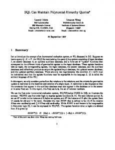
closed under polynomial-time conjunctive reductions there exists a leaf language L in V and a NDTM M such that on an input hx1 , . . . , xn i M produces a leafstring from L if and only if M0 produces on every input xi a leafstring from L0 . We will show T · ∃ · Leaf P (L0 ) ⊆ Leaf P (WL ) for the language WL with markers a, b. We proceed as before: whenever D queries the oracle ∃ · K with question t, N branches into two computations: – On the left branch, N produces a path for each possible witness wi of membership of t. However, instead of immediately verifying that the pair ht, wi i lies in K, our simulation simply assumes this hypothesis, postpones its check and resumes the simulation of D assuming a positive answer to the query. – On the right branch, N continues the simulation of D assuming a negative answer to the query. Once a branch of N ’s simulation of D terminates, we need to check that all input/witness pairs along that branch do lie in K. For this, N again branches into two paths: 14

a

exists y

in K ?

yes

(no questions) a leaf word in L

no

on every y

acc.

exists y’

in K ?

yes

no

acc.

rej.

b on every y’

questions all in K ?

a

−− leaf word for L −−

questions all

in K ?

−− leaf word for L −−

Fig. 3. Building a computation tree for the leaf language WL

– On the left path it produces a computation tree whose leafstring lies in L if and only if all input/witness pairs on that branch lie in K. This can be done because we assumed the closure under conjunctive reductions of Leaf P (V). – On the right branch it writes a marker a if D has accepted on this path of assumed oracle answers, and a marker b in the other case. Once again, if we consider the leafstring of N , we observe that the first subword wi sitting between two markers and lying in L indicates the valid computation of D. Accordingly, the marker which lies at the right of wi is a if and only if D accepts its input and this is precisely what the constructed language WL guarantees. This shows T · ∃ · Leaf P (L0 ) ⊆ Leaf P (WL ) and so, by Lemma 9 we conlude T · ∃ · Leaf P (L0 ) ⊆ Leaf P (UPol(BPol(V))). (b) follows from the construction in part ⊇ above. q.e.d. We define a sequence Di of languages for i ≥ 2 as follows. First D2 = 0∗ a{0, a, b}∗ , the language we used in the previous lemma. For k ≥ 3, we inductively define Dk+1 = WDk . Note that D2 lies in ∆L 2 and so we have Dk ∈ ∆k using Lemma 9. 15

Theorem 11 (Main). For every k ≥ 2: p Leaf P (Dk ) = Leaf P (∆L k ) = ∆k . p Proof. We establish Leaf P (Dk ) = Leaf P (∆L k ) = ∆k by induction on k. For k = 2, we have already shown in the previous proof that ∆p2 ⊆ Leaf P (D2 ) ⊆ Leaf(∆L 2 ). Furthermore, by Corollary 8 we get p p P Leaf P (∆L 2 ) ⊆ T · Leaf (DD 1 ) ⊆ T · BC · Σ1 = ∆2 .

For the induction step, we get: P L Leaf P (∆L k+1 ) = Leaf (Upol(BPol(∆k ))) (See Figure 1)

= T · ∃ · Leaf P (∆L k ) (Lemma 10) = T · ∃ · ∆pk = ∆pk+1 (from the induction hypothesis) p Note that we can indeed apply Lemma 10: by induction we have Leaf P (∆L k ) = ∆k which is closed under conjunctive reductions. We also get from Lemma 10 that P P Leaf P (∆L k+1 ) = Leaf (WDk ) = Leaf (Dk+1 ). q.e.d.

We should note that Meyer and Stockmeyer made the somewhat uncanonical p p choice of defining ∆pk+1 as T · Σkp rather than Πk+1 ∩ Σk+1 , probably because p this makes ∆k+1 a “syntactic” class [Pa94]. This has the advantage of allowing a nice completion of the correspondence between the dot-depth and polynomial hierarchies, in the line of Theorem 4. In Lemma 10, the technical condition that V contains the sub-alphabets is in fact superfluous: if V is a variety of languages whose syntactic monoids are groups and such that Leaf P (V) is closed under conjunctive reductions then we indeed have Leaf P (UPol(BPol(V)))) = T · ∃ · Leaf P (V). Handling of that case requires only a slightly different construction both for WL and for the simulation of the T · ∃ · Leaf P (L)-machine as well as extra algebraic considerations. In [ST03], it was shown that the class of regular languages which can be defined by twovariable sentences using ordinary and modular quantifiers is exactly the class DA ∗ G sol = UPol(BPol(Gsol )) where Gsol denotes the class of languages whose syntactic monoid is a solvable group. Our results combined with [HL*93] show Leaf P (DA ∗ Gsol ) = T · ∃ · Leaf P (Gsol ) = T · ∃ · M OD ∗ P where MOD∗ P denotes the closure of P under the Modq operators. Similarly, for any prime q, let Gq be the class of languages whose syntactic monoids are q-groups: we can show Leaf P (UPol(BPol(Gq )))) = T · ∃ · Leaf P (Gq ) = T · ∃ · M ODq P. All these results relativize and this allows us to shed new light on the problem of finding a leaf-language upper bound for BPP: the classical result of Lautemann 16

and Sipser (see [Pa94]) shows that BPP is contained in Σ2p ∩ Π2p and it is natural to ask whether there is a language L in Σ2L ∩ Π2L with BPP ⊆ Leaf P (L). This we now know cannot be the case with respect to all oracles since we will have Leaf P (L) ⊆ ∆p2 whereas relativized worlds exist in which ∆p2 is strictly contained in BPP (see e.g. [BT00]). Straubing and Th´erien have conjectured that BPP sits in Leaf P (UPol(BPol(Gsol ))) but there exist relativized worlds in which T · ∃ · ⊕P does not contain BPP [BT00] and it is perhaps possible to further show that in this world even T · ∃ · MOD∗ P does not contain BPP. Such a result would rule out any relativizable proof of the aforementioned conjecture.

6

Conclusion

We have shown that the Delta classes of the dot-depth hierarchy and of the polynomial hierarchy correspond via leaf-languages. This result also holds if we consider the Brzozowski definition of the dot-depth hierarchy. This extension of our result can be obtained using the “bridging” method outlined e.g. in [Pi98] which relates the two hierarchies in a straightforward way. We know by Theorem 11 that there are languages in ∆L 2 , for example D2 , that capture the class ∆p2 . Using algebraic methods, one can prove that if L is in p P P ∆L 2 then either Leaf (L) ⊆ BC(NP) or Leaf (L) = ∆2 but we do not know if a similar phenomenon occurs for k ≥ 3. A related question is whether the Dk languages which we defined are complete for the ∆L k -classes with respect to the reductions defined in [SW03]. For all varieties considered in this paper, we do have that Leaf P (V) is closed under polynomial-time conjunctive reductions and this can perhaps be concluded simply using the closure properties of the varieties. This would make Lemma 10 “cleaner” because it would shift the technical requirements to the class of languages V, with no requirements left for the complexity class Leaf P (V). We already mentioned that we could not find an example of a ∗-variety of languages V such that the opposite direction of Corollary 8 does not hold via oracles, i.e. such that T · Leaf P (V) is a proper subset of Leaf P (UPol(V)). Could it be the case that UPol and T· generally correspond on ∗-varieties of languages via leaf languages, without any conditions on the ∗-varieties of languages? Finally, when does a complexity class Leaf P (V) for a positive ∗-variety of languages V contain a language L such that Leaf P (V) = Leaf P (L)? The classes P Leaf P (ΣkL ), Leaf P (ΠkL ), and Leaf P (∆L k ) do have one, the classes Leaf (DD k ) P and Leaf (SF) seem not to. Is there, for example, an algebraic property which corresponds to this distinction? Acknowledgments. We thank Jean-Eric Pin for his help with Table 1. The fourth and fifth authors were supported by the Alexander von Humboldt foundation. 17

References [BGS75] T. P. Baker, J. Gill, R. Solovay Relativizations of the P =? NP Question, SIAM Journal on Computing 4, 1975, pp. 431-442 [BKS99] B. Borchert, D. Kuske, F. Stephan: On existentially first-order definable languages and their relation to NP, Theoret. Informatics Appl. 33, 1999, pp. 259–269 p [BSS99] B. Borchert, H. Schmitz, F. Stephan: Leaf P (∆B 2 ) = ∆2 , unpublished manuscript, 1999 [BS97] B. Borchert, R. Silvestri: A characterization of the leaf language classes, Information Processing Letters 63, 1997, pp. 153-158 [BCS92] D. P. Bovet, P. Crescenzi, R. Silvestri: A uniform approach to define complexity classes, Theoretical Computer Science 104, 1992, pp. 263–283. [BT00] H. Buhrman, L. Torenvliet, Randomness is Hard. SIAM J. Comput. 30(5): 1485-1501 (2000) [BV98] H.-J. Burtschick, H. Vollmer: Lindstr¨ om Quantifiers and Leaf Language Definability, International Journal of Foundations of Computer Science 9, 1998, pp. 277-294. [He84] H. Heller: Relativized Polynomial Hierarchies Extending Two Levels Mathematical Systems Theory 17, 1984, pp. 71-84. [HL*93] U. Hertrampf, C. Lautemann, T. Schwentick, H. Vollmer, K. Wagner: On the power of polynomial-time bit-computations, Proc. 8th Structure in Complexity Theory Conference, 1993, pp. 200–207. [Ka88] J. Kadin: The Polynomial Time Hierarchy collapses if the Boolean Hierarchy collapses, SIAM Journal of Computing 17, 1988, pp. 1263–1282. [MS72] A. R. Meyer, L. J. Stockmeyer: The equivalence problem for regular expressions with squaring requires exponential space, Proceedings 13th Annual IEEE Symposium on Switching and Automata Theory, 1972, pp. 125–129. [Pa94] C. Papadimitriou: Computational Complexity, Addison Wesley, Reading MA, 1990. [Pi98] J.-E. Pin: Bridges for Concatenation Hierarchies, Proc. ICALP, 1998, pp. 431–442. [PST88] J.-E. Pin, H. Straubing, D. Th´ erien: Locally trivial categories and unambiguous concatenation, Journal of Pure and Applied Algebra 52, 1988, pp. 297– 311. [PW97] J.-E. Pin, P. Weil: Polynomial closure and unambiguous product, Theory of Computing Systems 30, 1997, pp. 383–422. ¨tzenberger: Sur le produit de concatenation non ambigu, Semi[Sch76] M. P. Schu group Forum 13, 1976, pp. 47–75. [Sel01] V. L. Selivanov: Relating Automata-Theoretic Hierarchies to ComplexityTheoretic Hierarchies, Proc. FCT, 2001, pp. 323–334 [SW98] H. Schmitz, K. W. Wagner, The Boolean hierarchy over level 1/2 of the Straubing-Th´erien hierarchy, Technical report 201, Inst. f¨ ur Informatik, Uni. W¨ urzburg, 1998. [SW03] V. L. Selivanov, K. W. Wagner, A Reducibility for the Dot-Depth Hierarchy, Technical Report 313, CS Department, University of W¨ urzburg, December 2003 [St94] H. Straubing: Finite Automata, Formal Logic, and Circuit Complexity, Birkh¨ auser, Boston, 1994.

18

H. Straubing, D. Th´ erien, Regular Languages Defined by Generalized FirstOrder Formulas with a Bounded Number of Bound Variables, Theory Comput. Syst. 36(1), 2003, pp. 29-69. [TT02] P. Tesson, D. Th´ erien: Diamonds are forever: the Variety DA, in Semigroups, Algorithms, Automata and Languages, WSP, 2002, 475–499. [Wa90] K. W. Wagner: Bounded Query Classes, SIAM Journal on Computing 19, 1990, pp. 833–846 [Yao85] A. C.C. Yao: Separating the Polynomial Hierarchy by oracles, Poc. 26th IEEE Symp. on the Foundations of Computer Science, 1985, pp. 1–10 [ST03]

19