The Dynamic Applied Regional Trade (DART) Model A non-technical model description
Sonja Peterson∗ & Gernot Klepper, Kiel Institute for the World Economy Abstract: The DART model is a multi-sectoral, multi-regional dynamic computable general equilibrium model of the global economy developed for the analysis of international climate policies. Since the first version of DART was developed at the Kiel Institute for World Economics in 1998, the model has undergone a number of changes to run on more recent data and to analyze prevailing issues in international climate policies. The aim of this paper is to provide a brief non-technical model description.
∗
Sonja Peterson
Kiel Institute for the World Economy 24100, Germany Phone/Fax: +49-431-8814-406/522
[email protected]
1
Introduction
The DART Model of the Kiel Institute for the World Economy (IfW) is a recursive dynamic computable general equilibrium model of the global economy, covering multiple sectors and regions. It is designed for the analysis of economic issues associated with climate change and in particular for the analysis of international climate policies. The DART model stands, as the EPPA model of the MIT (Yang et al. 1996), in the tradition of the GREEN model by the OECD (Burniaux 1992), even though the models differ in several aspects. The first version of DART was developed in the late 1990’s and based on the data from the Global Trade Analysis Project (GTAP) in its Version 3 for 1993. The model was then used to simulate the implementation of the Kyoto Protocol via unilateral action (e.g. emission taxes) (Springer 1999) as well as to investigate the impacts of international capital mobility (Springer 2000; Springer 2002). In addition DART was coupled to an ocean-atmosphere model to assess the economic impacts of climate change (Deke et al. 2001; Kurtze and Springer 1999). Since then the model has been updated and extended several times and now runs on the GTAP6 data for 2001. Newer applications include the the analysis role of hot air in the Kyoto Protocol (Klepper and Peterson 2005) and the European emissions trading scheme Klepper & Peterson (2004, 2006). DART was also used to analyze whether marginal abatement costs curves derived from the the model can give good approximations of the outcome of emissions trading (Klepper and Peterson 2006). In the following we describe the general functioning and assumptions of DART.
2
The Basic-Model
The basic model, called Dynamic Applied Regional Trade (DART) is a multi-region, multi-sector general equilibrium model of the world. It is written in the mathematical programming language GAMS and currently based on the GTAP6 data set. The 57 sectors and 87 regions of GTAP6 can be aggregated depending on the question at hand. Currently DART is used with a 11-sector aggregation and different regional aggregations covering from 12 to 23 regions (see Table 1). Among the 11 sectors are 1
Table 1: Dimensions of DART Production sectors/Commodities
Energy Sectors
Non-Energy Sectors
COL
Coal
AGR
Agricultural Products
CRU
Crude Oil
IMS
Iron Metal Steal
GAS
Natural Gas
CEM
Chemical Industry
OIL
Refined Oil Prod.
PPP
Pulp and Paper Industry
EGW
Electricity
Y
Other Manufactures & Services
MOB
Transportation
Countries and regions
Annex B
WEU disaggregation
USA
USA
AUT
Austria
WEU
West European Union
BEN
Belgium & Luxemburg
OAB
Canada, Australia,
MED
Mediteranian (Greece, Cyprus, Malta)
New Zealand
SCA
EU Scandinavia (Finland, Denmark,Sweden)
JPN
Japan
FRA
France
FSU
Former Soviet Union
DEU
Germany
EEU
Eastern Europe
ESP
Spain
GBR
United Kingdom
Non-Annex B
BAL
Baltic Countries
LAM
Latin America
IRL
Ireland
IND
India
ITA
Italy
PAS*
Pacific Asia
POL
Poland
CPA
China, Hong Kong
NLD
Netherlands
MEA*
Middle East, N. Africa
PRT
Portugal
AFR*
Sub-Saharan Africa
EEU
Eastern EU (CZE, HUN, SVK, SLV, RMN, BUL)
*In EU-Aggregation aggregated to ROW - Rest of the World
2
three fossil fuel production sectors, different energy intensive sectors, agriculture, and other manufactures and services. Differentiating carbon intensive industries from noncarbon intensive industries allows to depict carbon intensity differences in production among regions and to cover the scope for substitutability across carbon-intensive goods and hence the potential for terms of trade effects caused by carbon abatement policies. The dynamic framework is recursively-dynamic meaning the evolution of the economies over time is described by a sequence of single-period static equilibria connected through capital accumulation and changes in labor supply. In this paper a non-technical description of the static and dynamic part of the DART model is provided. For an algebraic description of the original version of DART that is in most parts transferable to the current version, see Springer (1998). The economic structure of DART is fully specified for each region and covers production, investment and final consumption by consumers and the government. Primary factors are labor, capital, land and resources. All factors are in the basic version of DART intersectorally mobile within a region, but cannot move between regions. Fossil fuel resources are specific to fossil fuel production sectors, i.e. coal, natural gas and crude oil, in each region. Land is only used in the agricultural sector and in fixed supply. Each market is perfectly competitive. Output and factor prices are fully flexible. The following sections describe the producer and consumer behavior, foreign trade, factor markets and finally the calculation of carbon dioxide emissions, that are the basis for climate policy analysis.
2.1
Producer Behavior
Producer behavior is characterized by cost minimization for a given output. All industry sectors are assumed to operate at constant returns to scale. For the non-fossil fuel industries, a multi-level nested separable constant elasticity of substitution (CES) function describes the technological possibilities in domestic production1 . Figure 1 shows the nested production structure. On the top level of the 1 The
nesting structure and nest elasticities of the production cost functions are based on the ETA-
MACRO model (Manne and Richels 1992, pp. 130).
3
production function is a linear function, i.e. a Leontief function of non-energy intermediate goods and a value added composite2 . The intermediate input of good i in sector j corresponds to a so-called Armington aggregate of non-energy inputs from domestic production and imported varieties. The value added composite is a CES function of the energy aggregate and the aggregate of the primary factors. On the lowest level labor substitutes with capital in a Cobb-Douglas technology. On the output side, products destined for domestic and international markets are treated as imperfect substitutes produced subject to a constant elasticity formation.
»
¾ Export good Px
½
»
¾ Domestic used good Pd
2
CET ¼ ½! a ! aa τ =2 aa !! ! aa ! a!! » ¾
¼
Output Py
¾
½ !a aa ¼ !! ! aa !! a Leontief3 ! ! » ¾ aa
»
Composite Input Energy-Capital-Labor
Other intermediate Inputs
½ ¼ ½ ¼ 3 ´Q ´Q Q4 ´ ´ Q Leontief ´ CES Q ´ Q ´ σ = 0.5 Q ´ Q ´ Q Q ¾´ »¾ »
P a1 . . . P ai . . . P aN −1
Energy Composite
½
1 2
3 4
5
Value-added Composite
¼½ ¼ ¶S5 Cobb-Douglas ¶ S ¶ » S ¶ » S ¾ ¾ ¾ » ¾ »
CES4 ¶S σ = 0.75 ¶ S
Not investment good FossilElectrConstant elasticity of Capital Labor city fuels transformation τ ½ ¼ ½ ¼ ½ ¼ ½ ¼ ´Q Leontief: Fixed Coefficients ´ Q4 Constant elasticity of CESQ σ = 1.5 ´ ´³ Q Q ¶´ ¶ ³ ¶ ³ substitution σ Cobb-Douglas: σ = 1 Coal Gas Oil
µ
´ µ
´ µ
´
Figure 1: Production Structure of the Non Fossil Fuel Industry Sectors
2 In
the case of refined oil products, the intermediate input of crude oil and refined oil products are
also on the top level.
4
Export good Px
½
¾
»
¾ a aa
»
Domestic used good Pd
1
CET ¼ ½! ! τ =2 aa !! ! aa ! a!! ¾ »
¼
Output
¾
COL, GAS, OIL ½! ¼ aa ! !a 2 a ! CES aa !! σ = 0.75¾ aa !! »
Resource Rent
½
»
Macro Good
Composite ½ ¼ ´Q Leontief3 ´ Q ´ Q ´» Q Q » » ¾ ´ ¾ ¾
¼
Energy Oth. interm. Value-added Composite inputs Composite
½ ¾ Domestic used good P dcgd
½ ¾
¼ ½
¼ ½
¼
» 1 ¼ Constant elast. of transformation τ 2 Constant elast. of substitution σ »3
Leontief: Fixed Coefficients
Output Pcgd ½ ¼ 3 ´Q ´ Q Leontief ´ Q ´ Q ´ Q
P a1 . . . P ai . . . P aN −1
Figure 2: Production Structure of the Fossil Fuel Sectors and the Investment Good
The differentiation between energy and non-energy intermediate products is useful in the context of climate change policy. Energy use in production and consumption produces varying amounts of the greenhouse gas (GHG) carbon dioxide (CO2 ) depending on the fossil fuel source and the policies assumed to be in place. CO2 , with large emission levels, and a long lifetime in the atmosphere is the largest single contributor to the greenhouse effect. The other GHGs methane, nitrous oxide, ozone and halocarbons, as well as emissions from CO2 deforestation are sofar not considered in the model. The fossil fuels gas, coal and crude oil are produced from fuel-specific resources and the macro good (a composite of all other manufactures and services and factors). The production function is a CES function with a fixed factor - the fuel resource (see Figure 2). 5
In each region composite investment is a Leontief aggregation of Armington inputs by each industry sector. In the basic version of DART there are neither sector-specific investments nor cross border investment activities, i.e. investment goods are treated as non-tradables. Investment does not require direct primary factor inputs. Figure 2 shows the production structure of the investment activity. Producer goods are directly demanded by final consumers, comprising regional households and governments, the investment sector, other industries and the export sector.
2.2
Consumption expenditure
The representative household, that comprises private households and the government sector, receives all income generated by providing primary factors to the production process. After deducting taxes and savings, the disposable income is used for maximizing utility by purchasing goods. The final consumer decides between different primary energy inputs and non-energy inputs depending on their relative price in order to receive its consumption (utility) with the lowest expenditures. A fixed share of income is saved in each period. These savings are invested in the production sector. The expenditure function of the representative household is assumed to be a Cobb-Douglas composite of an energy aggregate and a non-energy bundle. Within the non-energy consumption composite, substitution possibilities are described by a Cobb-Douglas function of Armington goods. Figure 3 shows the structure of consumer behavior. »
¾
Final consumption ½ ¼ !!aaa ! 1 a !! Cobb-Douglasa !! ! a ¾ » ¾ aa » Other Armington Energy Composite intermediate inputs ½ ¼½ ¼ ´Q Cobb-Douglas1 ´ Q ´ Q ´ Q ´ Q 1 Cobb-Douglas: σ = 1
P ac1 . . .P aci . . . P acN
Figure 3: Final Consumption Production Structure 6
2.3
Foreign Trade
The world is divided into economic regions, which are linked by bilateral trade flows. All goods are traded among regions, except for the investment good. Following the proposition of Armington (1969), domestic and foreign goods are imperfect substitutes, and distinguished by country of origin. Import demand is derived from a three stage, nested, separable CES cost or expenditure function respectively and distinguishes between imported and domestically produced goods as well as between the country of origin. The structure of foreign trade is shown in Figure 4. The imports of one region r are equivalent to the exports of all other regions rr into that region r including transport. Transport costs, distinguished by commodity and bilateral flow, apply to international trade but not to domestic sales. The exports are connected to transport costs by a Leontief function on the third level. International transports are treated as a worldwide activity which is financed by domestic production proportional to the trade flows of each commodity. There is no special sector for transports related to international trade. »
¾ Armington Good Output
¾
¾
½ ©H ¼ H © 2 © CES HH © σ=4 ©© » ¾HH
»
Import Composite Domestic Output ½ ©H ¼½ ¼ © 2 H CES HH ©© σ = 8 ©© ¾ HH » »
Export Composite of
Export Composite of
region 1 to region r region H-1 to region r ½ ¼ ½ ¼ 2 2 ¡@ Leontief ¡@ Leontief ¡ @ ¡ @ @ @ ¾¡ » ¾ » ¾¡ » ¾ » Export of region 1
½ 1 2
Internat. Transport
¼ ½
Export of region H-1
¼ ½
Internat. Transport
¼ ½
¼
Constant elasticity of substitution τ Leontief: Fixed coefficients
Figure 4: Structure of Foreign Trade (Armington Production of Good i in Region r
7
On the export side, the Armington assumption applies to final output of the industry sectors destined for domestic and international markets. Here, produced commodities for the domestic and for the international market are no perfect substitutes. Exports are not differentiated by country of destination.
2.4
Factor markets
Factor markets are perfectly competitive and full employment of all factors is assumed. Labor is assumed to be a homogenous good, mobile across industries within regions but internationally immobile. In the basic version of the DART model capital is also intersectorally but not internationally mobile. Regional capital stocks are given at the beginning of each time period and result from the capital accumulation equation. In every time period they earn a correspondent amount of income measured as physical units in terms of capital services.
2.5
Carbon dioxide emissions
To calculate carbon dioxide emissions we follow the approach by Lee (2002) and multiply the physical quantity of gas, coal and crude oil used in either domestic production or domestic consumption (which is given in the GTAP data) with its emission coefficient and the fraction of carbon oxydized. DART uses the recommendations from the IPPC (1996) which are 0.0258 kgC/MJ for coal, 0.0153 kgC/MJ for gas and 0.2kgC/MJ for crude oil. The fraction of carbon oxydized is taken from Lee (2002). For gas and coal we directly receive the relevant emissions using this method. For oil emissions the calculation is more complicated. In order to determine the CO2 emissions which originate from the use of crude oil in the different production and consumption processes one needs to know at which point in the value-added chain this fossil fuel is actually burned, i.e. leads to emissions. In the current model crude oil only enters the production of refined oil products where it is not burned. Only refined oil products are burned as inputs in production or as final consumption goods. One cannot use the domestic use of crude oil for determining CO2 emissions since some of these oil prod8
ucts are exported and some are imported, hence there is no one-to-one correspondence between crude oil consumption and emissions. Since crude oil is the emission relevant input in refined oil production, only the crude oil share can be used for determining CO2 emissions. Refined oil consumption is composed of domestically produced and imported oil products. Both may have different carbon contents due to different input shares of crude oil in the production of refined oil products. The crude oil share in the production of oil products in region R is given by Crush(R) =
vaf m(CRU, OIL, R) vdm(OIL, R) + vxm(OIL, R)
i.e. the quantity of crude oil in refined oil production, denoted here vaf m(CRU, OIL, R), as a share of the value of the output of refined oil products (domestic vdm(OIL, R) and exports vxm(OIL, R)). Now, a regional carbon coefficient CEC(R) can be calculated as the crude oil share in oil products which are burned in that particular region R: CEC(R) = ¢ ¡ P vdm(OIL, R) ∗ Crush(R) + s [vxmd(OIL, S, R) ∗ Crush(S) ∗ 0.02 P s vxmd(OIL, S, R) + vdm(OIL, R) The denominator denotes all oil products which are used in region R. The nominator denotes the amount of crude oil in these products multiplied by the emission coefficient for crude oil.
3
Dynamics
The DART model is recursive-dynamic, meaning that it solves for a sequence of static one-period equilibria for future time periods connected through capital accumulation and changes in labor supply. The dynamics of the DART model are defined by equations which describe how the endowments of the primary factors capital and labor evolve over time. The major driving exogenous factors of the labor dynamic are population change, the rate of labor productivity growth and the change in human capital. The driving forces for capital accumulation are the savings rate and the gross rate of return on capital, and thus the endogenous rate of capital accumulation. The DART model is 9
recursive in the sense that it is solved stepwise in time without any ability to anticipate possible future changes, relative prices or constraints. The savings behavior of regional households is characterized by a constant savings rate over time. This rather ad-hoc assumption seems consistent with empirical observable, regional different, but nearly constant savings rates of economies, which adjust according to income developments over very long time periods (for savings rates see SchmidtHebbel and Serven 1997). Additionally, a wide range of empirical evidence in macroeconomic literature neglect the theoretically elegant permanent income hypothesis and shows that a huge fraction of the consumption decisions are based entirely on current after tax income. The following sections describe the evolution of labor and capital supply in more detail.
3.1
Labor supply
Labor supply considers human capital accumulation and is, therefore, measured in efficiency units, Lr,t . It evolves exogenously over time. Hence, labor supply for each region r at the beginning of time period t+1 is given by: ¯ r,t+1 = L ¯ r,t ∗ (1 + gpr,t + gar,t + ghr ) L where the bar denotes exogenous variables. An increase of effective labor implies either growth of the human capital accumulated per physical unit of labor, ghr , population growth, gpr , or total factor productivity, gar , or the sum of all. The standard version of DART assumes constant, but regionally different labor productivity improvement rates gar and declining population growth rates over time, gpr,t , according to the World Bank population growth projections. Because of the lack of data for the evolution of the labor participation rate in the future the growth rate of population instead of the labor force is used implying that the labor participation rate is constant over time. The human growth rates of human capital ghr are also assumed to be constant over time and regionally different. The 1990 levels of human capital endowments are taken from 10
Hall and Jones (1999)3 . They are then aggregated to the regions of the model. For the future development of the endowments, we assume that the maximum endowment of 12 years of schooling will be reached in 2050 and that this process starts at the computed 1990 levels and continues in a linear fashion. This approach can be be criticized as being rather ad-hoc. Since we could not identify a reasonable indicator for the future development of human capital endowments, we simply assumed optimistically that there is complete convergence in human capital intensities in the long run.
3.2
Capital formation
Current period’s investment augments the capital stock in the next period. The aggregated regional capital stock, Kst at period t is updated by an accumulation function equating the next-period capital stock, Kstt+1 , to the sum of the depreciated capital stock of the current period and the current period’s physical quantity of investment, Iqr,t . The equation of motion for capital stock Kstr,t+1 in region r is given by: Kstr,t+1 = (1 − δt )Kstr,t + Iqr,t where δt denotes the exogenously given constant depreciation rate. According to the GTAP5 data set δ is equal to 0.04, and we use the same value for all time periods. The allocation of capital among sectors follows from the intra-period optimization of the firms. As data on the regional physical capital stocks are not available with the GTAP data, the capital accumulation has to be rearranged by using physical capital earnings Kr,t i.e. return to capital, instead of the capital stock Kstr,t . Using the stock-flow-conversion, the capital earnings in period 0 for region r are given by Kr,0 = rkr,0 ∗ Kstr,t where rkr,0 denotes the gross rate of return on capital in region r in period 0 which is defined as rkr,0 = 3 The
Kr,0 pir,0 ∗ Kstr,0
countries missing from the 127 country data set of Hall and Jones are determined by taking
human capital intensity from a neighboring similar country.
11
pir,0 is the actual price of investment or in other words, the price of constructing a unit of capital. Exploiting the unit price convention pir,0 = 1 we can use rkr,0 as a (fixed) scaling factor. Thus, the capital accumulation equation can be rewritten in terms of physical units of capital services. (∗)Kr,t+1 = (1 − δt )Kr,t + Iqr,t ∗ pir,t ∗ rkr,0 where Kr,t denotes the physical unit of the factor capital in period t which earns 1$ in the initial time period and Iqr,t ∗ pir,t is the value of real gross investment. Once the variables have been scaled, the physical, i.e. quantity, units of capital services can be updated according to equation (∗); whereas the actual value of gross investment has to be scaled with the benchmark gross rate of return in every time period.
3.3
Dynamic Calibration
The dynamics of the DART model are driven by saving rates, population growth, and total factor productivity. For the capital accumulation we assume constant, but regional different saving rates. The rate for China allowed to adjust to income changes so that the originally high rates fall over time and become comparable to the saving rates in the other regions. This adjustment makes sure that China tends to converge towards a balanced growth path. Without these adjustments capital stocks will grow far beyond any realistic level with the consequence that either the rates of return on capital would collapse, or - if we introduce capital mobility - these regions would become major exporters of capital. Labor productivity rates are based on a thorough literature research on current estimates and adapted to reflect current projections of GDP growth. In addition, the assumption that the maximal human capital endowment will be reached in 2050 in the regions containing the developing countries leads to unrealistic high growth rates in LAM, MEA and AFR. We thus assume, that the maximal human capital endowment will only be reached in 2100. Table 2 summarizes the choice of the key parameters from the dynamics for the year 2001 on. 12
Table 2: Dynamic key parameters for selected regions for 2001 in %
Total growth in
techn.
Hum.
Popu-
Sav.
labor efficiency
progr.
capital
lation
Rate
USA
1.70
0.60
0.10
1.00
19.7
WEU
1.80
0.40
1.20
0.20
20.3
OAB
2.10
0.40
0.60
1.10
20.7
JPN
1.80
0.50
1.00
0.30
25.4
FSU
2.90
2.50
0.50
-0.10
22.3
EEU
3.20
2.5
0.90
-0.20
24.0
LAM
3.90
0.90
1.40
1.60
19.4
IND
6.10
1.70
2.70
1.70
22.2
PAS
6.10
2.10
2.50
1.50
22.3
CPA
5.20
3.40
1.90
0.90
34.5∗
MEA
4.40
0.80
1.50
2.10
20.8
AFR
5.10
1.00
1.90
2.20
18.3
*Falls by 0.5 percentage point per year up to 2010
Finally, the supply elasticities of fossil fuels are chosen in such a way that the carbon emission in 2030 resulting from the model in the business as usual scenario meet the projections of the World Energy Outlook 2004 (IEA 2004). The resulting elasticities for a regional aggregation without the WEU disaggregation are 0.94 for coal, 0.85 for gas and 0.98 for crude oil.
4
Concluding Remarks
This paper presents a brief model description of the dynamic multi-regional, multisectoral general equilibrium trade model DART. DART is a powerful tool to analyze international climate policies especially those associated with the Kyoto-Protocol and the European emissions trading scheme. As new issues become prevailing, DART will
13
be expended and augmented. Current projects include the inclusion on non-CO2 gases, the coupling of DART to GIS based land-use model for Germany and Europe to better analyze the role of land-use changes in climate policy and the better representation of technological change.
References Burniaux, J.-M. (1992). GREEN - a multi-sector, multi-region dynamic general equilibrium model for quantifying the costs of curbing CO2 emissions: a technical manual. OECD Working Paper, Economics Directorate, OECD, Paris. Deke, O., K. G. Hooss, C. Kasten, G. Klepper, and K. Springer (2001). Economic impact of climate change: Simulations with a regionalized climate-economy model. Kiel Working Papers No. 1065. Hall, R. E. and C. I. Jones (1999). Why do some countries produce so much more output than others? Quarterly Journal of Economics 114 (1), 83–116. IEA (2004). International Energy Outlook 2004. Klepper, G. and S. Peterson (2004). The EU emissions trading scheme: Allowance prices, trade flows, competitiveness effects. European Environement 14 (4), 201– 218. Klepper, G. and S. Peterson (2005). Trading hot air: The influence of permit allocation rules, market power, and the us withdrawal from the kyoto protocol. Environmental and Resource Economics 32 (3), 205–227. Klepper, G. and S. Peterson (2006). Marginal abatement cost curves in general equilibrium: the influence of world energy prices. Resource and Energy Economics 28 (1), 1–23. Kurtze, C. and K. Springer (1999). Modelling the impact of global warming in a general equilibrium framework. Kiel Working Papers 922, Kiel Institute for World Economics. Lee, H.-L. (2002). An emissions data base for integrated assessment of climate change policy using gtap. GTAP Workin Paper Draft, GTAP. 14
Manne, A. S. and R. G. Richels (1992). Buying Greenhouse Gas Insurance. Cambridge: MIT Press. Schmidt-Hebel, K. and L. Seren (1997). Saving across the world: Puzzles and policies. Discussion Paper 354, World Bank, Washington, D.C. Springer, K. (1998). The DART general equilibrium model: A technical description. Kiel Working Papers No. 883. Springer, K. (1999). Climate policy and trade: Dynamics and the steady-state assumption in a multi-regional framework. Kiel Working Papers No. 952. Springer, K. (2000). Do we have to consider international capital mobility in trade models? Kiel Working Papers No. 964. Springer, K. (2002). Climate Policy in a Globalizing World: A CGE Model with Capital Mobility. Kieler Studien. Berlin: Springer. Yang, Z., R. Eckaus, A. D. Ellerman, and H. Jacoby (1996). The MIT emissions prediction and policy analysis (EPPA) model. MIT Report 6, Massachusetts.
15