[12] K. Kyu-Ho, L. Yu-Jeong, R. Sang-Bong, L. Sang-Kuen, and Y. Seok-Ku, "Dispersed generator placement using fuzzy-GA in dis- tribution systems ... [25] S. P. Han, "A Globally Convergent Method for Nonlinear Pro- gramming," Journal of ...
The Effect of Distributed Generation Modeling and Static Load Representation on the Optimal Integrated Sizing and Network Losses M. F. AlHajri, Student Member, IEEE, and M. E. El-Hawary, Fellow, IEEE
ABSTRACT In this paper the impact of both the Distributed Generation (DG) modeling and the static load response to voltage upon the optimal DG size, the radial distribution real power losses, and on the resulting voltage profiles are investigated. The optimal DG sizing nonlinear programming problem is tackled by the Sequential Quadratic Programming deterministic technique. The DG modeling and the different static load representations were tested on 30–bus radial distribution system. Simulation results indicate that the DG size and network losses as well as voltage profiles are highly dependent on the DG and Load representations. Index Terms––Distribution Generation, Distribution Generation Modeling, Load Modeling, Sequential Quadratic Programming, Radial Distribution System. I. INTRODUCTION istributed Generation (DG) is a small and modular power electric generator, with an output ranging form 1 kW to 5 MW located at or near the load site at the distribution level [1]. DG is either interconnected to the distribution utility grid, directly to the customer side of the network or both. The DG is also referred to as on-site generation, dispersed generation, embedded generation, and decentralized generation. Dispersed generation, in particular, is customarily reserved for small DG power output units (1 kW–500 kW) [2]. Due to the latest improvement in the DG technology, a country like Denmark is relying on DG to supply 40 % of its electric power demand [3]. Globally, in 2005 the total installed wind power capacity was 59.1 GW, and it is expected to reach 134.8 GW by the year 2010 [4]. An EPRI study predicted that by the year 2010, 25% of the all new generating capacity will be captured by distributed power [5]. Another study provided by the Natural Gas Foundation concluded that the DG contribution to the newly installed generation would be in the vicinity of 30% [6]. DG includes technologies that are driven either by fossilbased fuel or by renewable energy. Backup diesel generators, Combined Heat and Power (CHP) gas turbines, micro-turbine and fuel cells are technologies of the fossil-fuel DG types. Wind turbines, small hydro power turbines, solar and photovoltaic cells are of sustainable energy DG types. Integrating DG into electric power networks has many benefits. These benefits greatly depend on where the DG is located and on its size [7;8]. Few examples of such benefits could be summed as follows:
D
1. 2. 3.
Improve the system voltage profiles, Reduce the power losses, Improve both reliability and efficiency of the power supply by reducing thermal stresses caused by loaded substations, transformers and feeders, 4. Deferring upgrades for an existing infrastructure by releasing the available capacity of the distribution substation, 5. Decrease Transmission and Distribution (T&D) related costs. In order to achieve the aforementioned benefits, the DG size has to be optimized. The optimal DG size is dealt with as a nonlinear programming (NLP) problem with both nonlinear objective function and constraints. Such DG NLP problem was solved via heuristic and deterministic techniques. The heuristic methods utilized in the attempt of solving the DG optimal size were Genetic Algorithm (GA) [9-11], hybrid GA–Fuzzy [12;13] and Particle Swarm Optimization [14]. However, the heuristic techniques tend to converge more slowly compared to their deterministic counterparts [15]. In this paper, the Sequential Quadratic Programming (SQP) deterministic method is utilized in solving for the optimal DG size due to its excellent reputation in solving nonlinear constrained optimization problems [16-18]. In the tested radial distribution system, the connected static loads are represented as constant power, constant current or as constant impedance models. The integrated DG is modeled as PQ–DG bus and PV–DG bus. Each DG model is tested and optimally sized against the three different static load representations. The impacts of different DG modeling and different static load representations upon the radial distribution network losses, voltage profiles and on the integrated DG rating are investigated. II. MATHEMATICAL FORMULATION The DG sizing problem is to be handled as a constrained nonlinear programming problem; that is both the objective function as well as the constraints are nonlinear. The objective function to be minimized is the radial distribution system real power losses, while the nonlinear constraints include equality, inequality and boundary constraints. The NLP problem constraints are as follows: 1. The equality constraints: Theses are the power flow equations that govern the power system. 2. The inequality constraints: Theses are the thermal constraints imposed on the system such as the equipments’ rating and the feeders’ ampacity limit.
978-1-4244-1643-1/08/$25.00 ©2008 IEEE 001543 Authorized licensed use limited to: Dalhousie University. Downloaded on December 24, 2009 at 22:58 from IEEE Xplore. Restrictions apply.
3.
The boundary constraints: These are the voltage limits dictated by system operator on both the magnitudes and phase angles.
A. The objective function The DG integration into a radial distribution system has several merits, and minimizing the real power losses is considered one of the important tasks of such installation. The DG NLP problem is expressed mathematically as follows:
would be 2 NB − ( 2 + nDG ) equations if the DG to be represented as a PV bus. Number ‘2’ refers to those of the radial distribution substation. The power flow equations to be fulfilled are expressed as follows: NB
j =1 NB
Minimize
j =1
s.t. hi ( x ) = 0
i = 1, 2,! , l
g j ( x) ≤ 0
j = 1, 2,! , m
(1)
x− ≤ x ≤ x+
(
)
where Gij : real part of the ijth element of the admittance matrix, Bij : imaginary part of the ijth element of the admittance matrix, YBus , nDG : number of proposed DGs th δ : angle of ij element of the admittance matrix. ij
where
f RPL ( x )
h( x ) g ( x) •+ •−
NB
x
C. The inequality constraints The inequality constraints demonstrate the thermal network design restrictions and they are manifested by lower and upper limits imposed on the real and reactive power flows in the radial distribution lines and distribution transforms as well as the feeders’ ampacity and the substation capacity limits. Such constraints can be accounted for as follows:
: is the network real power losses, : equality constraints, : inequality constraints, : the maximum permissible value, : the minimum permissible value, : number of radial distribution system buses
= ª¬ Vi =2:NB
T
δ i =2:NB
DGsize º¼ .
¦(P
nDG
where PDG
ª Rij cos δ ij f RPL ( x ) = ¦¦ « ( Pj Pi + Q j Qi ) i =1 j =1 « Vi V j ¬ NB NB
+
Rij sin δ ij V j Vi
º
(2)
( P Q − Q P )» j
i
j i
(5)
max {kVAij or kVAji } ≤ kVAijrated
(6)
DGi
: DG real power output i
QDG
: DG reactive power output,
kVAij
: branch ij apparent power flow, : branch ij maximum allowable apparent power flow
i
kVAijrated
»¼
)
+ jQDGi ≤ PS / S + jQS / S
i =1
The total radial distribution system active power losses dissipated in overhead lines, cables and distribution transformers is formulated as shown in (2) [19].
D. The boundary constraints The bus voltage magnitudes and phase angles are bounded by upper and lower limits imposed by the system operator. The DG power factor is allowed to operate at values between two extreme levels determined by the type and nature of the DG to be installed in the radial distribution network. Such restrictions are expressed mathematically as shown in (7)–(9).
where Rij : ijth real part element of the impedance matrix, Pi : net real power at bus i, Qi : net reactive power at bus i, Vi : bus i complex voltage • : magnitude of complex quantity,
δi δ ij
)
Qi − ¦ Vi Bij V j cos δ ij − Vi Gij V j sin δ ij = 0 (4)
f RPL ( x )
x
(
Pi − ¦ Vi Gij V j cos δ ij − Vi Bij V j sin δ ij = 0 (3)
: bus i voltage angle : phase angle difference, i.e.
Vi − Vo
δ ij = δ i − δ j
B. The equality constraints The highly nonlinear power flow equations are the equality constraints that must be satisfied throughout the process. In the radial distribution network, the power flow equations corresponding to the equality constraints would be of 2 NB − 2 equations if the DG is modeled as a PQ bus. On the other hand, the number of the power flow equality constraints
φi − φo pf
− DG
∞
∞
≤ξ+
(7)
≤ζ+
≤ pf DG ≤ pf
(8) + DG
(9)
Where
•o •
: the nominal value, ∞
: the infinity norm, x
∞
001544 Authorized licensed use limited to: Dalhousie University. Downloaded on December 24, 2009 at 22:58 from IEEE Xplore. Restrictions apply.
= max
i =1,2,!, NB
(x ) i
pf DG
: DG operating power factor. III. SOLUTION METHODOLOGY
A. Sequential Quadratic Programming The nonlinear DG sizing problem is handled via SQP methodology. SQP is one of the primal numerical search methods that directly solve the original constrained problem. The SQP algorithm models Lagrangian function of the constrained nonlinear optimization problem by a Quadratic Programming (QP) subproblem. The transformed subproblem is solved at a k
given approximate solution, x , to determine a search direction at each major iteration. The step size, calculated by minimizing a descent function along the search direction, is joined with the QP subproblem solution to construct a new iterate with a better solution, x
k +1
. The process is repeated in *
an iterative manner until an optimal solution, x , is met or certain criteria are satisfied. For that, SQP is also sometimes called Recursive Quadratic Programming (RQP) or Successive Quadratic Programming [20]. The QP subproblem is formulated by using the secondorder Taylor’s expansion to approximate the objective function and the first-order Taylor’s expansion to linearize the equality and the inequality constraints as follows:
1 Minimize ∇f RP ( xk )T d + d T H k d 2 s.t.
the Inaccurate Line Search methods, and popular descent functions are suggested by [22;24;25]. Both the number of gradient evaluations and the subproblem dimension are significantly reduced by incorporating the active set strategy. The active set strategy includes all the equality constraints and only a subset of the inequality constraints; i.e. those that are either active or violated inequality constraints. SQP is not a single algorithm but rather a sophisticated collection of algorithms that collaborate in the endeavor of searching for an optimal solution. Most general purpose optimization commercial software utilize the SQP technique in solving a large set of practical nonlinear constrained optimization problems [26]. B. Static Load Representation Accurate and proper load modeling is of significant concern in power distribution systems as well its transmission systems counterpart [27;28]. Loads in electric power system are usually expressed by adequate representations so as to mimic their effects upon the system. The load dependency on the operating bus voltage and on system frequency or both are among those representations. Static loads are generally not affected by frequency [29]. In this paper the voltage dependency of static load characteristics is considered. Thus, the static loads in the distribution system are represented by exponential or polynomial models. The exponential model is shown in (12) and (13), while the polynomial model is expressed in (14) and (15).
(10)
α
§V · P = Po ¨ ¸ © Vo ¹
∇hi ( xk ) d + hi ( xk ) = 0 T
∇g j ( xk )T d + g j ( xk ) ≤ 0
§V · Q = Qo ¨ ¸ © Vo ¹
where d is the search direction, together with the step size the next approximated solution is obtained as xk +1 = xk + α k d k [21]. By using the curvature information in determining the search direction, the algorithm’s rate of convergence is improved. The search direction is obtained by applying the Karush-Khun-Tuker conditions on the Lagrangian function for the problem defined in (10) and solving the corresponding equations. The Lagrangian function would be written as
1 L = ∇f RPL ( xk )T d + d T H k d + 2 l
¦ λ ∇h ( x )
T
i
i
k
d + hi ( xk ) +
(11)
i =1 m
¦ β ∇g j
j
( xk )T d + g j ( xk )
j =1
H , the Hessian matrix, is approximated and updated by the modified [22] Broyden-Fletcher-Goldfarb-Shanno (BFGS) [23] Quasi-Newton method which uses only the first order information. The step size, �, can be determined by an appropriate merit or descent function that ensures reducing the objective function of a minimum optimization problem type while satisfying all the constraints. Practical descent functions are based on
(12) β
2 § § V ·2 · §V · ¨ P = Po a p ¨ ¸ + bp ¨ ¸ + c p ¸ ¨ © Vo ¹ ¸ © Vo ¹ © ¹ 2 2 § §V · · §V · Q = Qo ¨ aq ¨ ¸ + bq ¨ ¸ + cq ¸ ¨ © Vo ¹ ¸ © Vo ¹ © ¹
(13)
(14)
(15)
Vo is the nominal voltage; V is the operating voltage; while Po and Qo are the active and reactive parts of the consumed load consumed at the nominal voltage. For the polynomial model, a p + bp + c p = aq + bq + cq = 1 . Symbols � and � are the values of exponents which determine the load characteristics. Specific � and � values lead to a specific lode model. That is, 1. If � and � are both zero, the model represents constant power characteristics; 2. If � and � are both one, the model represents constant current characteristics; 3. If � and � are both two, the model represents the impedance characteristics. 4. Certain load components would be represented by fractional exponents, refer to [30] for details.
001545 Authorized licensed use limited to: Dalhousie University. Downloaded on December 24, 2009 at 22:58 from IEEE Xplore. Restrictions apply.
1.05
Voltage Profiles For No DG and DG cases 1.03 Constant Power
No DG
Constant Current
Constant Impedance
1.01 Voltage (pu)
C. Modeling Distribution Generation Units The DG will be treated as a PV bus and PQ bus models in the tested radial distribution system. The PV---DG model represents a DG which is capable of delivering active power as well as a reactive power that keeps the terminal voltage at a specific value determined by the system operator. The PQ---DG model, on the other hand, delivers real power at a designated power factor. Whilst the DG can be modeled in a PV---control mode[8], most DG penetration buses are represented as a PQ buses in the distribution system [31]. Both representations are adopted and their impact on the network real power losses is investigated in this research. It is customary for the DGs to operate at a power factor between 0.85�and unity [7]. The PQ model of the DG source is represented as a negative load delivering a real and reactive power to the distribution system regardless of the system voltage. The PV model is dealt with as a negative active power with negative sufficient reactive power needed to hold the DG bus at a definite value.
sults are shown in Table II. The impact of modeling the DG as a PV bus on the voltage profile is manifested in Fig. 3 and 4.
0.99 0.97
0.95 0.93
0.91 1
2
3
4
5
6
7
8
9 10 11 12 13 14 15 16 17 18 19 20 21 22 23 24 25 26 27 28 29 30 Distribution Bus Numbe r
Fig. 1. Voltage profile with and without PQ–DG installation.
1
Voltage Profile for the three Load Models 0.995
Voltage (pu)
In an effort to achieve optimal DG integration into radial distribution system and obtaining reliable results, the system loads are to be modeled properly. The polynomial is not considered in this research, and the loads are to be expressed using the exponential models. That is, the DG is to be optimally integrated into the radial distribution system with the static loads represented as constant power, constant current or constant impedance models. The DG size is investigated for all three cases in the endeavor of finding the optimal and practical integration.
Constant Power
Constant Current
Constant Impedance
0.99
0.985
0.98
0.975 1
2
3
4
5
6
7
8
9 10 11 12 13 14 15 16 17 18 19 20 21 22 23 24 25 26 27 28 29 30 Distribution Bus Number
IV. TEST RESULTS AND DISCUSSION
Fig. 2. Voltage profile with PQ–DG integrated for the three load models.
Integrating a single DG into a typical urban distribution system is investigated thoroughly and the SQP nonlinear optimization method is used to determine its optimal rating. The tested radial network consists of 30 buses with 20 loads connected. The system is configured of one main and two long lateral. The first and the second laterals have 9 and 11 branches respectively. The urban distribution system full data can be obtained from [32]. This system has a total active and reactive power demand of 3.2 pu and 1.6 pu respectively. The nonlinear constrained optimization problem simulations were carried out within MATLAB® computing environment using HP®, AMD® Athlon® 64x2 Dual Processor 5200+, 2.6 GH and 2 GB of memory desktop computer. For the 30–bus test system, the following cases were considered: • Case 1: In this case, a single DG is modeled as a PQ bus and placed at bus number 10 to optimally minimize the radial distribution real power losses. The 20 connected static loads are represented as either constant power, constant current or constant impedance model in each run and the optimal DG size is obtained consequently. Table I shows the DG real and reactive power outputs as well as the computed real power losses. Fig.1 and 2 shows voltage profiles for the tested system at the pre-DG and post-DG installation situations. • Case 2: the procedure of case 1 is repeated with the DG is modeled as a PV bus. The corresponding re-
Results shown in Table I and II and in Fig. 1–4 clearly indicate that placing the DG into a distribution system minimized the real power losses and improved the voltage profile. The pre–DG installation lowest voltage was 0.9147 pu at bus 17; whereas the lowest voltage is obtained after integrating a PQ– DG model with loads represented as constant power as 0.9816 pu at bus 29. Results show that by modeling the DG as a PV bus, the network real power losses were lower than their counterpart in the PQ model. Moreover, the optimal PV–DG sizes are higher than the PQ–DG sizes. Among the static load representations, the constant power load modeling yields the lowest losses and voltage profiles for both DG modeling, PQ–DG or PV–DG. Fig. 5 shows a flowchart that illustrates the results achieved by modeling the DG and the connected loads. TABLE I RESULTS OF DG INTEGRATION AS A PQ BUS MODEL
Load Modeling Constant Power Constant Current Constant Impedance
DG Power (pu) 1.3704 1.3944 1.4227
001546 Authorized licensed use limited to: Dalhousie University. Downloaded on December 24, 2009 at 22:58 from IEEE Xplore. Restrictions apply.
DG Reactive Power (pu) 0.8493 0.8641 0.8817
Power Losses 0.1044 0.1080 0.1123
1.06 Voltage Profiles for No DG and DG cases Costant Power
Voltage (pu)
1.03
Constant Current
Constant Impedance
No DG
1
0.97
0.94
0.91 1
2 3
4
5
6 7
8
9 10 11 12 13 14 15 16 17 18 19 20 21 22 23 24 25 26 27 28 29 30 Distribution Bus Numbers
by represented the DG to be integrated by the PQ–DG model the size was lower than its counterpart with comparable volte profiles. The losses though were higher than that of the voltage controlled DG bus model. For the static load representation, it was found that the constant impedance model resulted in the highest losses for both DG models and the constant power representation produced the lowest network losses. This study shed some light on the pros and cons for both DG models which might be of assistance when decision is to be made.
Fig. 3. Voltage profile with and without PV–DG installation.
VI. REFERENCES [1]
1 0.999
Voltage (pu)
0.998
[2]
0.997
[3]
0.996 0.995 0.994
[4]
Voltage Profiles for the Three Load Modeles 0.993 Constant Power
Constant Current
Constant Impedance
[5]
0.992 2
3
4
5
6
7
8
9 10 11 12 13 14 15 16 17 18 19 20 21 22 23 24 25 26 27 28 29 30
[6]
Distribution Bus Numbers
Fig. 4. Voltage profile with PV–DG integrated for the three load models. TABLE II RESULTS OF DG INTEGRATION AS A PV BUS MODEL DG Power DG Reactive Power Losses Load Modeling (pu) Power (pu) (pu) Constant Power 1.7861 1.1069 0.0699 Constant Current 1.7945 1.1121 0.0701 Constant Impedance 1.8030 1.1174 0.0704
[7]
[8]
[9]
DG Models
[10] PV-DG
PQ-DG
Network Real Power Losses
Optimal DG Size
Network Real Power Losses
Optimal DG Size
Constant Power Model
0.0699 pu
1.7861 pu
0.1044pu
1.3704 pu
Constant Current Model
0.0701pu
[11]
[12] 1.7945 pu
0.1080 pu
1.3944 pu
[13] Constant Impedance Model
0.0704pu
1.8030 pu
0.1123 pu
1.4227 pu
[14] Fig. 5. Flowchart shows the obtained results.
V. Conclusion In this paper, SQP technique was utilized in investigating the impact of both DG models and the static load representation on the DG optimal size, network losses and voltage profiles. It is found that the PV–DG model yields a higher DG size but lower real power loses and better voltage profiles. However
[15] [16]
[17]
EPRI TR-111490, "Integration of Distributed Resources in Electric Utility Systems: Current Interconnection Practice and Unified Approach," Electric Power Research Institute-EPRI-Palo Alto, CA,1998. F. A. Farret and M. G. Simões, Integration of Alternative Sources of Energy Wiley-IEEE Press, 2006. P. Djapic, C. Ramsay, D. Pudjianto, G. Strbac, J. Mutale, N. Jenkins, and R. Allan, "Taking an Active Approach," IEEE Power & Energy Magazine, vol. 5, no. 4, pp. 68-77, 2007. Global Wind Energy Council (GWEC) , http://www.gwec.net/, 2007. "Installation, operation, and maintenance costs for distributed generation technologies," EPRI, Palo Alto, CA,2003. N. Hatziargyriou, M. Donnelly, S. Papathanassiou, J. A. Pecas Lopes, M. Takasaki, H. Chao, J. Usaola, R. Lasseter, A. Efthymiadis, K. Karoui, and S. Arabi, "CIGRE technical brochure on modeling new forms of generation and storage," CIGRE, TF 38. 01. 10, November, 2000. P. P. Barker and R. W. De Mello, "Determining the impact of distributed generation on power systems. I. Radial distribution systems," IEEE Power Engineering Society Summer Meeting, vol. 3, pp. 1645-1656, 2000. T. Niknam, A. M. Ranjbar, and A. R. Shirani, "Impact of distributed generation on volt/Var control in distribution networks," IEEE Power Tech Conference Proceedings, vol. 3, p. 7, 2003. E. Haesen, M. Espinoza, B. Pluymers, I. Goethal, V. Thongh, J. Driesen, R. Belman, and B. de Moor, "Optimal placement and sizing of distributed generator units using genetic optimization algorithms," Electrical Power Quality and Utilisation Journal, vol. 11, no. 1 2005. N. Mithulananthan, T. Oo, and L. V. Phu, "Distributed Generator Placement in Power Distribution System Using Genetic Algorithm to Reduce Losses," The Thammasat International Journal of Science and Technology, vol. 9, no. 3, pp. 55-62, 2004. M. G. Ippolito, G. Morana, E. R. Sanseverino, and F. Vuinovich, "Risk based optimization for strategical planning of electrical distribution systems with dispersed generation," IEEE Bologna Power Tech Conference Proceedings, Bologna, vol. 1, p. 7, 2003. K. Kyu-Ho, L. Yu-Jeong, R. Sang-Bong, L. Sang-Kuen, and Y. Seok-Ku, "Dispersed generator placement using fuzzy-GA in distribution systems," IEEE Power Engineering Society Summer Meeting, Chicago, IL, USA, vol. 3, pp. 1148-1153, 2002. M. Gandomkar, M. Vakilian, and M. Ehsan, "A Genetic-Based Tabu Search Algorithm for Optimal DG Allocation in Distribution Networks," Electric Power Components and Systems, vol. 33, pp. 1351-1362, Dec.2005. M. F. AlHajri, M. R. AlRashidi, and M. E. El-Hawary, "Hybrid Particle Swarm Optimization Approach for Optimal Distribution Generation Sizing and Allocation in Distribution Systems," 20th Canadian Conference on Electrical and Computer Engineering, BC, Canada, pp. 1290-1293, 2007. "http://reference.wolfram.com/ mathematica/ tutorial/ ConstrainedOptimizationGlobalNumerical.html," 2007. P. T. Boggs, "Sequential Quadratic Programming," in Acta Numenca (1995). A. Iserles, Ed. Cambridge University Press, 1995, pp. 1-51. M. S. Bazaraa, H. D. Sherali, and C. M. Shetty, Nonlinear Programming: Theory and Algorithms, 3rd ed Wiley-Interscience, 2006.
001547 Authorized licensed use limited to: Dalhousie University. Downloaded on December 24, 2009 at 22:58 from IEEE Xplore. Restrictions apply.
[18] [19] [20] [21] [22]
[23] [24] [25]
[26] [27] [28]
[29] [30] [31]
[32]
J. Nocedal and S. Wright, Numerical Optimization, 2nd ed Springer, 2006. O. I. Elgerd, Electric Energy Systems Theory: An Introduction, 1st ed Mcgraw-Hill, 1971. P. T. Boggs and J. W. Tolle, "Sequential Quadratic Programming," Acta Numerica 1995, pp. 1-51, 1995. J. S. Arora, Introduction to Optimum Design, 1st ed Mcgraw-Hill College Division, 1989. M. J. D. Powell, "A fast algorithm for nonlinearly constrained optimization calculations," Numerical Analysis, G. A. Watson ed. , Lecture Notes in Mathematics, vol. 630/1978, pp. 144-157, 1978. P. E. Gill, W. Murray, and M. H. Wright, Practical Optimization, 1 ed. London: Academic Press, 1981. B. N. Pshenichny, "Algorithms for the general problem of mathematical programming," Kibernetica, vol. 5, pp. 120-125, 1978. S. P. Han, "A Globally Convergent Method for Nonlinear Programming," Journal of Optimization Theory and Applications, vol. 22, p. 297, 1977. "http://www-fp.mcs.anl.gov/otc/Guide/," 2007. C. Mo-Shing and W. E. Dillon, "Power system modeling," Proceedings of the IEEE, vol. 62, no. 7, pp. 901-915, 1974. IEEE Task Force on Load Representation for Dynamic Performance, "Bibliography on load models for power flow and dynamic performance simulation," IEEE Transaction on Power Systems, vol. 10, no. 1, pp. 523-538, 1995. J. Arrillaga and B. Smith, AC-DC Power System Analysis Inspec / IEE, 1998. C. W. Taylor, Power System Voltage Stability Singapore, McgrawHill, 1993. W. H. Kersting and R. C. Dugan, "Recommended Practices for Distribution System Analysis," IEEE PES Power Systems Conference and Exposition, pp. 499-504, 2006. S. Rajagopalan, "A New Computational Algorithm for Load Flow Study Of Radial Distribution System," Computer and Electric Engineering, vol. 5, pp. 225-235, 1978.
001548 Authorized licensed use limited to: Dalhousie University. Downloaded on December 24, 2009 at 22:58 from IEEE Xplore. Restrictions apply.