1
The Effect of Pipeline Depth on Logic Soft Errors Eric L. Hill, Member, IEEE, and Mikko H. Lipasti, Senior Member, IEEE
Abstract—Soft errors arising from particle strikes to combinational logic circuits can be masked logically (by dominant inputs), electrically (the pulse is too weak to flip a node), or by opportune timing (the transient pulse arrives at a downstream latch when the latch is opaque). The latter effect—timing-window masking—is commonly approximated analytically by computing the ratio of the length of the latching window to the cycle time. This paper identifies the shortcomings of this analytical approach, and highlights the potential for drawing an intuitively attractive but incorrect conclusion from such a model: that deeplypipelined, high-frequency circuits are increasingly vulnerable to logic soft errors. We show empirically that this is not the case, and advocate the use of mean work to failure, or MWTF, instead of MTTF, to accurately describe the vulnerability of pipelined circuits. Furthermore, we identify a second-order effect—SET fanout—which increases the error-resilience of deep pipelines over their shallower counterparts, in effect reversing the previously-held intuition. Index Terms—Combinational logic circuit fault tolerance, pipeline processing, computer reliability
I. I NTRODUCTION In this paper, the relationship between clock frequency and reliability is explored. Increasing clock frequencies are commonly cited as one of the reasons that soft errors in logic are becoming an important design concern [1][2]. The relationship between the frequency a circuit is clocked at and its soft error rate is intuitive, as shortening the clock cycle time of a circuit decreases the probability that a SET is timing window masked. The experiments described in this paper show that this intuition is in fact flawed, and that the vulnerability of a logic block to soft errors is largely independent of the degree to which it is pipelined. These experiments also show that combinational gates within more aggressively pipelined circuits are more resilient to the effects of transient faults. This study also uncovers two key observations which not only explain these surprising results, but also serve to refine conventional intuition regarding the proper manner in which to make fair comparisons of reliability, and the appropriate level of modeling detail required to obtain realistic results. The first key result produced by this study is that the direct comparison of soft error rates is not always the appropriate manner in which to evaluate the reliability of different logic blocks. Herein, we outline the scenarios where direct rate comparisons are inappropriate. Furthermore, the results presented in this paper also underscore the importance of modeling the effects of timing window masking explicitly. The use of analytical models for timing window masking [1][3][4], obscures second Manuscript received January 8, 2010. This work was supported by NSF grant CCF-0702272. Eric L. Hill was with University of Wisconsin–Madison when this work was performed. He is now with Intel Corp. (e-mail:
[email protected]). Mikko H. Lipasti is with University of Wisconsin–Madison (e-mail:
[email protected]).
order effects which can significantly impact the error rates of combinational logic. The remainder of this paper is divided into three sections. In the first section, conventional intuition regarding how logic soft error rates scale with clock frequency is defined formally. The next section identifies the flaws in this intuition and proposes methodological refinements in order to address these flaws. The final section of this paper presents analysis on synthesized functional units using this refined methodology and discusses the implications of the results. II. C ONVENTIONAL I NTUITION A. Combinational Logic Soft Error Rates A bit flip only occurs as a result of a particle strike on a combinational logic gate when the generated SET logically propagates to the input of a flip-flop and changes the value captured. In order for this to happen the SET has to arrive at the flip-flop data input during the rising edge of the clock. In the cases where a SET arrives at the input of a flip-flop, but not when the rising edge occurs, the SET is said to be timingwindow masked. The expression shown in Equation 1 was proposed by [1] to analytically determine the probability that the arrival of a SET at the input of a flip-flop would coincide with the rising edge of the clock. (d - w) (1) C Equation 1 expresses this probability as the function of 3 quantities: the SET duration d, which in this work is the amount of time the amplitude of the pulse is above or below Vdd/2, the latching window w, which is the sum of the setup and hold times for the flip-flop, and the clock period C. From this equation it is simple to infer the first-order effect of increasing the pipeline depth of a unit on the combinational logic soft error rate. At deeper pipeline depths, C decreases, implying an increase in Tderating . Simply put, the value of Tderating (and thus the overall error rate) should be inversely proportional to the clock period. Tderating =
B. Latch Soft Error Rates In addition to being vulnerable to particle strikes on combinational logic gates, errors in computation can also occur when bits are flipped as a result of direct strikes on storage cells within flip-flops. It is assumed in this work that all flipflops considered are constructed of back to back level sensitive latches. Seifert et al. characterized the vulnerability of latches to particle strikes, finding that latches are only vulnerable to bit flips in opaque mode [5]. A latch in transparent mode is not vulnerable because it is being driven by fan-in logic. If it is assumed that the waveform used to clock the circuits has a 50% duty cycle, this implies that each latch is only vulnerable
to a particle strike 50% of the time. When the pipeline depth of a functional unit is doubled, the first order intuition is that the latch count (and thus the latch area) should also double, implying a proportional increase in the latch soft error rate. III. C HALLENGING THE C ONVENTIONAL I NTUITION When deeper pipelines are blamed for increasing soft error vulnerability, one issue that is often overlooked is that the stated intuition only holds when comparing error rates. In the literature, system reliability is commonly quantified in terms of a error rate λ (and its reciprocal MTTF). Directly comparing error rates of two systems is only valid when both systems take the same amount of time to complete a task. Ultimately, the impact of errors on a system is represented by the product of the failure rate and the time the system is running, as shown by equation 2. errors observed = λ * time
(2)
Despite the fact that MTTF is generally accepted as a standard reliability metric, it is not adequate for comparisons when two systems have different failure rates and running times. A. A Hypothetical Example To illustrate how comparing error rates directly does not always result in a fair comparison, consider the two functional units shown in Table I. This table shows two logic blocks which are identical in functionality. Additionally, Unit A is purely combinational, while Unit B is pipelined into 2 stages. The clock periods for Unit A and Unit B are set to 1 and 0.5 time units, respectively. Additionally, both units have the same amount of area devoted to logic, while Unit B has the twice the latch area. Because the two units are functionally the same, it is valid to make the assumption that approximately the same fraction of faults are logically masked by each circuit. Given this, the analytical expression for timing derating, shown in Equation 1 can be leveraged, allowing the combinational logic soft error rate to be approximated in this example as being proportional to the reciprocal of the clock period. In a similar manner, the latch error rate should be proportional to the latch area.
Pipestages Clock Period Logic Area Latch Area Logic Error Rate Latch Error Rate
Unit A
Unit B
1 1 1 1 1 1
2 0.5 1 2 2 2
TABLE I: Hypothetical Functional Unit Descriptions. All values shown in terms of arbitrary units.
B. Scenarios Where Rate Comparison is not Appropriate In the context of combinational logic SER, these assumptions imply that the error rate should be dependent only on the
Fig. 1: Timing Diagram for Instruction Processing.
timing component of the derating factor. From this, it follows that the error rate of Unit B should be twice that of Unit A, due to its shorter clock period. If error rates are used as a direct comparison here, the conclusion would be that Unit A is more reliable, since its longer clock period allows more particle strikes to be timing-window masked. Consider the scenarios shown in Figure 1. This figure is designed to illustrate the ways that each unit described in Table I could complete four arbitrary units of work over time. The top portion of this diagram depicts how these four units of work would be completed over time by Unit A. The lower portions of this figure depict two different ways Unit B could complete the same amount of work. These two cases represent scenarios where Unit B is not and is the execution bottleneck, respectively. In all cases, the x-axis represents time (in arbitrary time units), while the y-axis (for each of the three scenarios) represents the status of a particular pipe-stage. Colored and blank regions represent periods of time where a particular pipe-stage is computing or idle, respectively. In the case where Unit A is processing this work, all four time units are needed, so the 1 pipe-stage in that particular circuit is always busy. In this case the expression 1*4T (it takes four time units for unit A to complete the work shown in Figure 1, at an error rate of 1) represents the total number of errors that would be observed for Unit A. In contrast to this, consider the scenario shown in middle of Figure 1. In the case where Unit B is not the performance bottleneck units of work will arrive for processing at the same rate as the scenario shown for Unit A. In this case, despite the fact that it takes the same amount of time to complete the task on both units, Unit B will be idle half of the time. This is illustrated in Figure 1 by the unshaded regions in the timing diagram. Because particle strikes are uniformly distributed across time, only half of the strikes on Unit B will hit pipe-stages computing valid results. A similar situation occurs in the third scenario depicted, where Unit B is the system bottleneck, and units of work arrive and are processed as fast as possible. In both of these cases, the expression 2*2T represents the number of errors that would be observed (it takes two time units to complete the work, at an error rate of 2). To summarize, when only rates are compared, Unit A will be chosen as the more reliable design, as it has an error rate of 1, while Unit B has an error rate of 2. In contrast, when the amount of errors observed is used as a comparison
metric, 4T errors will be observed in both cases implying that Unit A and Unit B are equivalent in terms of reliability. A similar situation arises in the context of latch SER. The increase in error rate due to the area increase should also be offset by the shortened amount of time it takes to complete the assigned work. C. Using the Right Metric As was stated previously, MTTF is a widely used metric for reliability. It is typically calculated as the ratio total time MTTF = number of errors encountered which simplifies to
(3)
1 total time = (4) λ * total time λ Comparisons using this metric have the implicit assumption that the total time required to perform computation in each system is identical. This is not the case for our functional unit comparison, meaning that MTTF is not the correct metric to use. Weaver et. al more recently proposed an alternative reliability metric, mean instructions to failure (MITF) [6]. MITF is calculated as the ratio MTTF =
instructions committed number of errors encountered which simplifies to MITF =
UWPC * freq UWPC * total time * freq = (6) λ * total time λ The original work proposing MITF expressed the metric in terms of instructions per cycle (IPC), as the work was proposed in the context of considering the effects of soft errors in microprocessor. In the context of this discussion MITF is expressed in terms of units of work per cycle (UWPC), where a unit of work is described as the amount of work done in a single pipe-stage of Unit A or B. The implicit assumption made by this metric is that the default unit of work (an “instruction” in [6]) is consistent across all systems being compared. In our comparison, the unit of work is not consistent. One unit of work for Unit A is equivalent to two units of work for Unit B. In order to accurately compare system with inconsistent units of work, Reis et. al proposed a more generalized metric, mean work to failure (MWTF) [7]. This metric was originally proposed to provide fair comparisons of reliability across dissimilar architectures, which might have inconsistently defined units of work. MWTF is defined as the ratio amount of work completed number of errors encountered
(7)
which simplifies to amount of work completed (8) λ * execution time This metric takes a more abstract definition of what constitutes a unit of work. It also factors in the difference in execution time for different systems. For this metric, typically something MWTF =
4 1 = λ * 4T T and MWTF for Unit B would be
(9)
1 4 = (10) 2 * λ * 2T T Which is the result expected from the previous discussion. D. Revised Intuition The application of the appropriate metric, MWTF, to evaluate the effects of pipelining a functional unit make it clear that to a first order an increase in pipeline depth should have no effect on the SER. Several experiments were conducted to explore this revised intuition. IV. E XPERIMENTAL S ETUP
(5)
MITF =
MWTF =
larger (like a transaction or an entire benchmark) is used as the basis for a unit of work. This broader definition allows for consistency across systems that may be very different. For the purposes of our comparison, it is best to define a unit of work, as one item processed by Unit A. This means that (looking at the diagrams in 1 and 1) that both Unit A and Unit B are doing 4 units of work (even though Unit B completes the work in 8 clock cycles rather than 4). Applying this metric, the MWTF for Unit A would be
In order to further explore the revised intuition developed in the previous section, several fault injection experiments were performed, using the methodology described in [8]. For this particular study, floating point addition and multiplication units based on the designs from the UltraSPARC T1 were chosen as benchmarks [9]. These units were chosen because nearly every general purpose microprocessor has floating point hardware. In addition to this, the decision of whether or not to fully pipeline a unit (which affects the frequency at which the unit is clocked), often comes up in the design of floating point hardware. Generating several comparison points for evaluation required the creation of multiple versions of each unit, pipelined to varying degrees. In order to create these benchmarks, all flip-flops within the behavioral Verilog representation of these units were removed, creating purely combinational versions of each logic block. These combinational logic blocks were then synthesized to LSI 10k standard cells using Synopsys Design Compiler, and re-timed using the automatic pipelining functionality within the synthesis tool chain. This process yielded 2 stage, 4 stage, and 8 stage pipelined versions of each original circuit. The attributes of each benchmark circuit are shown in Table II. The clock periods shown in this table were obtained by taking the measured critical path delay for each 8 stage design, and doubling that value successively as the number of pipeline stages is halved. While it is unlikely that the actual critical path delay would double when the number of stages is halved, the premise of this study was to consider a system where in the nominal case a functional unit is fully pipelined (into 8 stages in this case) and to explore how making the unit not fully pipelined affected reliability. The last column of Table II reports the flip-flop area percentage in the context of drain regions vulnerable to particle strikes. Statistical fault
Fig. 2: Combinational Logic Soft Error Fault Model.
Fig. 4: Measured Overall Logic Derating of Floating Point Units.
Fig. 3: Flip-Flop Soft Error Fault Model.
injection was performed on each benchmark, with 100,000 particle strikes being simulated in each case.
Benchmark
Clock Period
flip-flops
% FF area
fpadd comb fpadd 2stg fpadd 4stg fpadd 8stg fpmul comb fpmul 2stg fpmul 4stg fpmul 8stg
3040 1520 760 380 3120 1560 780 390
104 419 1123 2463 83 389 2269 3598
1.1% 4.0% 9.9% 18.5% 0.3% 1.5% 8.1% 12.1%
TABLE II: Description of Benchmarks Used for Pipeline Depth Study.
Diagrams of all possible outcomes that can occur when transient faults are injected into combinational logic gates and flip-flops are shown in Figures 2 and 3, respectively. Using these fault models, the derating factor for combinational logic faults is calculated by taking the sum of outcomes C and F divided by the total number of faults injected. Similarly for errors injected directly into flip-flops, derating is calculated by dividing the sum of outcomes C and E by the total
Fig. 5: Plot of Logic Derating Adjusted for Execution Time.
number of faults. For each benchmark circuit studied, separate experiments were performed injecting faults exclusively into combinational gates, and then flip-flops. V. C OMBINATIONAL L OGIC SER The graphs shown in Figure 4 plots the measured derating for faults injected into combinational logic for each of the floating point units studied. The graph shown in Figure 5 plots the same data, except adjusting to account for the execution time differences that would exist between pipeline configurations. From this figure it is clear that the results of this experiment do not match our revised intuition. Instead of staying constant, the measured derating actually decreases as pipeline depth increases, when adjusted for execution time. The propagation of SETs to multiple flip-flops along unbalanced paths is responsible for this counterintuitive result, and is only observable when the effects of timing window masking are modeled A. SET Fanout Effects A diagram describing the second order effect responsible for the counterintuitive results in Figure 5 is shown in Figure
Fig. 6: Illustration of SET Fanning out to Multiple Flip-flops.
Fig. 7: Experimental Measurement of Effective SET Width.
6. In the scenario depicted in Figure 6, transient pulses fan out from a single combinational logic gate to two downstream flip-flops. In this case, the path length and delay from the gate to each flip-flop is different. In this situation, the absolute window of time where at least one flip-flop could be corrupted is lengthened. This new window of time was defined as the effective SET width. This quantity is illustrated in Figure 6 as the superposition of the SETs arriving at each flip-flop. The equation shown in Equation 1 to characterize timing derating can be written as shown in Equation 11 to account for the impact of this second order effect. effective SET width - w (11) C The average effective SET width observed during several fault injection experiments was measured and plotted for different pipeline configurations in Figure 7. For our experiments, the average transient width of an injected SET is 100 ps. From this figure it is clear that at the shallower pipeline depths, the SET fanout effect is significantly more pronounced. The effect is more pronounced in these pipeline configurations because there is the same amount of combinational logic, but fewer flipflops, implying that a transient will have to propagate through more levels of logic (and thus fan out further) before reaching a flip-flop. Tderating =
VI. L ATCH SER In Figure 8, the overall latch error rates are plotted for both floating point units across all considered pipeline configurations. This error rate was measured experimentally by using the formula shown in Equation 12. For this calculation, all area values used are normalized to the combinational case (where the only latches present in the circuit are for the primary outputs). latch error rate = (normalized area) ∗
FFPO + FFERR (12) faults injected
Looking at this plot, it is clear that the soft error rates (specifically for the multiplier unit) more than double when the pipeline depth is increased by a factor of 2. The adder circuit
Fig. 8: Measured Normalized Latch Soft Error Rate.
has results similar to what was predicted by the previously developed intuition, having a roughly 2X increase going from combinational to two, two to four, and four to eight pipeline stages. In contrast, there is a 4X increase observed in the measure latch soft error rate going from the two stage to four stage cases. This unexpected growth in the observed soft error rate can mainly be attributed to a larger than expected growth in latch count, as can be observed in Table II. VII. C OMBINED SER The combined SER (latch + logic) adjusted for execution time is plotted in Figure 9. This was calculated by weighting the latch and logic derating values by their respective areas, and multiplying by the execution time for each particular pipeline configurations. The execution times are normalized to the combinational case. Because the majority of vulnerable area in all comparison points shown can be attributed to combinational logic gates, the effects described in the previous section have a profound effect on the scaling of the soft error rate. This is especially true for the shallower pipeline depths, where not only a larger fraction of area can be attributed to logic, but
[6] C. Weaver, J. Emer, S. S. Mukherjee, and S. K. Reinhardt, “Techniques to Reduce the Soft Error Rate of a High-Performance Microprocessor,” SIGARCH Computer Architecture News, vol. 32, no. 2, p. 264, 2004. [7] G. A. Reis, J. Chang, N. Vachharajani, R. Rangan, D. I. August, and S. S. Mukherjee, “Design and Evaluation of Hybrid FaultDetection Systems,” in Proceedings of ISCA-32, 2005. [8] E. L. Hill, M. H. Lipasti, and K. K. Saluja, “An accurate flipflop selection technique for reducing logic ser,” in DSN. IEEE Computer Society, 2008, pp. 128–136. [9] S. Microsystems, “OpenSPARC T1 Microarchitecture Specification,” August 2006.
Fig. 9: Combined SER Adjusted for Execution Time.
also SET fanout affects (conceptually illustrated in Figure 6) are reducing the amount of timing window masking. For the deeper pipeline depths, increasing latch area means the latch soft error rate has a larger influence on the overall error rate observed. VIII. C ONCLUSION In this paper, the effect of pipelining logic, commonly cited as a reason the logic soft error problem is being exacerbated, was explored. In this exploration, the fallacy in this line of thinking (the use of MTTF as a comparison metric) was uncovered, and the correct metric to use, MWTF, was identified. The newer MWTF metric was used to refine the previously cited conventional intuition to having the soft error vulnerability of a circuit be independent of pipeline depth, rather than directly proportional to it. In validating this revised intuition, a second order effect causing adjusted failure rates to decrease at deeper pipeline depths was uncovered. The use of the correct comparison metric (MWTF), along with this second order effect, SET fanout, mean that deeper pipelines are in many cases more resilient that their shallower counterparts, reversing the previously held intuition. R EFERENCES [1] P. Shivakumar, M. Kistler, S. W. Keckler, D. Burger, and L. Alvisi, “Modeling the Effect of Technology Trends on the Soft Error Rate of Combinational Logic,” in DSN ’02: Proceedings of the 2002 International Conference on Dependable Systems and Networks, 2002. [2] G. Saggese, A. Vetteth, Z. Kalbarczyk, and R. Iyer, “Microprocessor Sensitivity to Failures: Control vs. Execution and Combinational vs. Sequential Logic,” in Proceedings of DSN, 2005. [3] M. O. Bin Zhang, Wei-Shen Wang, “FASER: Fast Analysis of Soft Error Susceptibility for Cell-Based Designs,” in Proceedings of ISQED 2006, April 2006. [4] N. Miskov-Zivanov and D. Marculescu, “MARS-C: Modeling and Reduction of Soft Errors in Combinational Circuits,” in DAC ’06: Proceedings of the 43rd annual conference on Design automation, 2006. [5] N. Seifert and N. Tam, “Timing vulnerability factors of sequentials,” in IEEE Transactions on Device and Materials Reliability, vol. 4, no. 3. IEEE Computer Society, 2004, pp. 516–522.