The Effects of Communication Latency Upon ... - Semantic Scholar

Purdue University

Purdue e-Pubs Computer Science Technical Reports

Department of Computer Science

10-18-1990

The Effects of Communication Latency Upon Synchronization and Dynamic Load Balance on a Hypercube Dan C. Marinescu John R. Rice

Marinescu, Dan C. and Rice, John R., "The Effects of Communication Latency Upon Synchronization and Dynamic Load Balance on a Hypercube" (1990). Computer Science Technical Reports. Paper 34. http://docs.lib.purdue.edu/cstech/34

This document has been made available through Purdue e-Pubs, a service of the Purdue University Libraries. Please contact [email protected] for additional information.

THE EFFECTS OF COMMUNICATION LATENCY UPON SYNCHRONIZATION AND DYNAMIC LOAD BALANCE ON A HYPERCUBE

Dan C. Mariocscu Jobo R. Rice CSD-TR-I032 September 1990

The Effects of Communication Latency Upon Synchronization and Dynamic Load Balance on a Hypercube* Dan C. Marinescu, John R. Rice Computer Science Department Purdue University

West Lafayette, IN

47907, U.S.A.

Abstract

In this paper we discuss the effects of the communication latency upon the dynamic load balance for computations which require global synChronization are discussed. Experimental results from the study of the performance of iteration methods on an NCUBE 1 are presented.

1

Introduction

In this paper, we are concerned with the effects of synchronization upon the performance of iterative methods on hypercubes. vVe restrict our discussion to the case when all PEs execute the same program, but on different data; the so-called SPMD paradigm. The SPMD paradigm is widely used today and it will probably continue to be so for large applications using tens of thousands of PEs, since it is fairly difficult to write and debug many different programs for the processing elements of a large system. The SP~I'ID execution implies that the same program and diITerent data sllb-domains are loaded in the local memory of the distributed memory multiprocessor. To obtain a large speedup, it is necessary to maintain a high processor utilization. The amount of time processors are idle needs to be kept as low as possible, so the load assigned to different processors must be balanced. A static load balancing in the SPMD execution means to assign to every PE balanced or equal data subdomains with the hope that during execution, different processors will have dynamic loads close to one another. But static load balancing does not provide a guarantee of dynam~·c load balancing. Due to data dependencies, the actual flow of control of different PEs will be different, different PEs will execute different sequences of instructions. Even the execution time of an instruction is data dependent. Hence starting computations at the same time on all PEs does not guarantee that they will terminate at the same time even when their loads are statically balanced. Synchronization is an important aspect of computing using message passing in a distributed memory multiprocessor system. There are numerous cases where synchronization is necessary. For example, iterative methods require synchronization since a processor has to exchange boundary \"alues with its neighbors, but only after all of them have finished their computation on the current iteration. Communication on a distributed memory machine is fairly expensive, the time to • Work supported in part by the Stra.tegic Defense Initiative through ARO gran ts DAAG03-86-I{-0106 and DAAL0390-0107, and in part by NSF grant Celt 56H1817.

1

exchange a short message between two nearest neighbors is typically equivalent to the time to e:x:ecute 10 2 floating point operations. It follows that synchronization, an operation which requires a consensus of all processors and involves the exchange of a large number of messages, is a source of considerable inefficiency. Observe that if the execution time on all PEs were perfectly equal, then synchronization would be unnecessary. It would suffice to start all the computations at the same time and all iterations will stay synchronized. Data dependencies make this approach unfeasible. If the study of data dependencies allows us to compute the load imbalance factor .6., (defined in [11]), then methods to reduce the effects of synchronization can be considered. For example, a method of self synchronization discussed in Section 6 proposes that every P E enters the communication period at the end of each iteration only after a time equal to Jl(l +.6.) with Jl the expected execution time per iteration. Then a synchronization takes place only every Rth iteration. From this brief presentation it follows that even if the effects of data dependencies are relatively minor and they may increase the actual execution time only by a few percent, their analysis is important in order to design schemes which prevent the frequent need for synchronization by requiring processors to enter periods of self blocking.

2

Communication Latency on a Hypercube

A simplified model of parallel computations with global synchronization is presented in [6]. A serious limitation of the model comes from the assumption that in epoch [;k all the h processing elements, 1l"1l ••• , 1l"h: start computing precisely at the same time and the epoch terminates when the last processor in the group completes its execution. Communication does not occur instantaneously, so concurrent start ups are not possible. On the contrary, the communication latency between any two processors 1l"; and 1l"j is substantial. For example, according to [2], the time to deliver a short message from node i to node j on an NCUBEj1 can be approximated by Oij

= 261

+ 193dij

with the transmission latency in J,lsec.

O;j

d ij

=

the Hamming distance between node i and node j. For example d 14 = 2 since 1 = 0001 and 4 = 0100. The distance dij represents the number of links to be traversed by a message from the source (i or j) to the destination (j or i) node.

When dij = 10 then we have Oij ~ 2200 J,lsec. The communication is faster on second generation hypercubes. For example on NCUBEj2 with a 20 MHZ clock, the time to deliver a short message (2 bytes) from node 1l"; node'1rj is approximately [lJ

12 20· 10 6 with

2

=

the transmission latency in JLsec.

140 Msec

is the start-up and the close-up time for a connection.

2 Jisec

is the overhead in routing the packet at every intermediate node along the path.

20· Mbps

the DMA transfer rate.

If di, = 10 then Oi, ~ 160Msec. Note that this approximation for OJ; does not take into account

possible contention for communication links and/or memory with other nodes, but it is an effective delivery time. It takes into account the software overhead associated with VERTEX, the operating system on NCUBE.

3

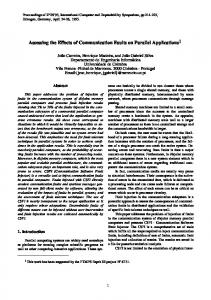
Synchronization and Broadcasting on a Hypercube

In this section, we assume that a sub-cube of dimension L is allocated to a computation C which requires global synchronization. Each processor executes the same code, but on different data according to the following pattern. A leader, usually processor 11'0, signals the beginning of an epoch and every P E, 11', starts computing and upon termination, signals completion. \¥hen ToO receives completion messages from all 11';, 1 ~ i ~ 2£ -1, the next epoch is started. To analyze quantitatively the effects of communication latency, it is necessary to define precisely the communication patterns involved in global synchronization. In this paper we consider a broadcast-collapse synchronization protocol using the broadcast tree shown in Figure 1. In this protocol, a synchronization epoch starts when tio broadcasts a short message signaling the beginning of the epoch. Each processor IT; starts computing as soon as it receives the start-up signal. Each processor sends up a termination signal to its ancestor in the tree when the following two conditions are fulfilled: (i) It has completed execution. (ii) It has received a termlnation signal from all its descendents (if any) in the broadcast tree. This protocol guarantees that ITo receives a termination signal if and only if all PEs have signaled termination and there is no contention for communication links, due to signaling of beginning and termination of the epoch. The tree in Figure 1 has the property that in a cube of order L the number n( of nodes at level e is

0:> e:> L. In other words, all nodes at distance e from the root are at level e. It follows that if the communication hardware has a fan-out mechanism which allows a node to send a broadcast message to all its immediate descendents at the same time, then the broadcast tree is optimal in the sense that each node receives a broadcast message from the root at the earliest possible time. If such a fan-out is not supported by the hard ware, then the following scheme guarantees that the node at the farthest distance from the root receives the broadcast message at the earliest possible time. Anode at level £ in the broadcast tree (see Figure 1) sends messages to its descendents at level l+ 1, in the order of the depth of the sub-tree routed at that node. For example, 11'0 sends the broadcast 3

I

! 1

Level I

Level'

..

" Level 3

.""

'0000

,,"',

UlOID 10100

loon 10110 10101 11001 11010 11100

Level 4

1111

10111 11011 Il1lo 11101

Level 5

1111\

FIGURE 1: A broadcast tree which allows optimal communication time in distributing or collecting messages.

4

messages in the following order 7l"t. 7l"2, "'10 71"8, 7l"16, since the subtrees routed at these nodes have their respective depth 4, 3, 2, 1 and O. To implement the synchronization protocol described earlier, each PE at level £ > 0 executes repeatedly the following sequence of steps: read start-up message from ancestor....atJevel (£ - 1) execute computation for i = 1, number..descendents-atJevel £ + 1 do begin read terminationJIlessage (*) end write terminationJIlessage to ancestor-atJevel £ - 1 This code assumes a blocking read and a non-blocking write. The generic read statement allows a node to read the termination messages in the order they arrive. If a generic read statement is not available, then the node at level £ has to read messages from its descendents at level £ + 1 to minimize blocking. An optimal strategy in this case is to read first from the node with the shortest subtree. For example, 7l"0 should read in the order 7l"16, 7l"s, 7l"4, "2, nl, since the corresponding subtrees have the depth 0, 1, 2, 3 and 4 respectively. Note that in this case the communication time for the collapse mechanism is dependent upon the number of descendents at distance one. A node may have at most L descendents and in our analysis we overestimate the time to read all termination messages as 01 = Lo' with 0' the time for a read operation which does not block, since the data is already there.

4

A First Order Approximation for the Effects of Synchronization Upon Efficiency

To estimate the effect of communication latency in global synchronization upon processor utilization, consider a very simple model based upon the following assumptions. Al

The computation C uses a sub-cube of dimension L of a hypercube of dimension N, and there is no interference between the sub-cube allocated to C and other sub·cubes. No messages other than those needed by C are routed through the sub-cube.

A2

The execution time of the computation allocated to every processor in epoch i is a constant E, 0 S i :s; 2£ - 1.

A3

A broadcast/collapse mechanism is used for synchronization. To signal the beginning of a synchronization epoch the processor at the root of the broadcast tree, S 7l"0 sends a message of the shortest length at time t and the message reaches the nt processors at level £ in the broadcast tree at time tt = is + £00. To signal the termination of the synchronization epoch, the processors at level L send a message of the shortest length at time time t£ = is + Loo + E and the message is processed by "0 at time lS' = is + E + L(oo + od. The timing diagram corresponding to this synchronization protocol is presented in Figure 2 for the case L = 5.

5

Lo

,, ,, ,,

,, ,, ,, ,, , ,,

"I

'. \

C"c''--

_

C"~8'--

_

"16

,, I , , , I , I ,

,, ,

11"24

,, ,, ,, ,, ,

1l'"20 11'18 1['17

,

: __---'' CIC''--__

L,

,

,

iLIO

:

C"C''--

:

:",5

:

"~6,---

__

"" "" "25 "" ""

""

1i13

"14

,

"n ",

,,

,, ,, ,, ,,

,, ,, ,,

iT27

il'23

"15

•

•

,, ,

""

,,,' ' , ,

Ls

~, 7r29

,

I'

,, ,, ,, ,, ,, ,, ,, ,, ,, ,, ,, ,, ,,

_

"3

,, ,, ,, ,, ,, ,, , ,, ,, ,, ,

L3

_

0

1 01

"31

,

tL =

E

., is

+ Loa

I"

1'+E+L(80 +81 )

FIGURE 2: A timing diagram for the case L = 5. Broadcast time per level collapse time per level is at. and the execution time is E.

6

IS

00,

Since we have assumed constant execution times and no communication interference from other sub-cubes, the synchronization protocol described above guarantees that no blocking due to memory and/or link contention will ever occur, and the duration of a synchronization epoch is precisely Ts = E + L(oo + Ot). Call 0 = 00 + 0t. It follows immediately that when assumptions A1-A3 are true, then the average utilization of any processor is

u=

E E+L8

E Ts

1 -

LO E+L8

DC

1

U= 1 -

= 1 -

E V;

1+

1 l+~

-5

with /3 = a factor describing the computation to communication time ratio. For example, when E = 1000, namely when the computation time is two orders of magnitude larger than communication time, then for a cube of order L = 10 it follows that /3 = 10 and U= 1 -

1 - '" 0.89. 11

When E = 0 then /3 = 0.1 and U :::: 0.09l. For the NCUBE/2 we have 0 ~ 160 jlsec, while the execution time of the fastest instruction is about 50 nanoseconds. It follows that in order to achieve 90% processor utilization on such a hypercube, each P E has to execute about 10 2 . 10 3 = 10 5 instructions in a synchronization epoch. The previous analysis can be easily extended to the case when the execution time has a bounded stastical distribution, Le., when the execution time Xi on 11"; satisfies a ::; Xi ::; b, and when the broadcast-collapse time per level satisfies 0 :2:: b-a. In this case it is guaranteed that communication latency hides all the effects of nondeterminancy in execution time. In other words, a processor at level f. will always complete its execution no later than the completion messages from all its descendents have arrived, as shown in Figure 2. Consider processors 1i" i and 1i"j with actual execution times a and b, respectively. To complete execution on 1rj before receiving aU the completion messages, say from 1i"j, in the worst case scenario we must have the condition b ::; 00 + 01 + a or 0 :2:: b - a. In this case, the processor utilization is bounded by 1 -

with

1+

1 (2 L _t)a+b

"U,,1

L

1 1

+ ~b

b ~b = L8 .

To minimize the inefficiency associated with low values of /3b, the following strategy could be used. Rather than assign equal computations to every PE, assign a higher load to processors at lower levels in the broadcast-collapse tree. For example, Figure 2 suggests that in the case of constant execution time E the processors at level f. can be kept busy for an additional time equal to

T/=(L-£)8. The computation time for processors at level

ecould then be 7

+ (L -

E, = E or

(1+

E, = E

L - 1] + Li3

1)0 = E [ 1 1

t)

~

This simply means that rather than having an equipartition of the data domain, an optimal balanced assignment would mean to assign different computational loads depending upon the position of the processor in the broadcast-collapse tree. With tms approach all nl. PEs at levell have a utilization

U = 1 _

£0

,

= 1 -

E+ Lo

1 1 - --. L 1 + il

The average utilization is

uapt

1 2"

and substituting for Ut we have 1 " -L: 2" '=0

uapt

(") £ -2- ] £ [1 L 1 + il

1

1 -

ltil

or

£2[.-1

UO" = 1 -

L2"

1

1

1

1 + il = 1 - 2" 1 + il

To evaluate the advantage of this approach, consider the case when

E =

o.

In this case, using an equipartltion of the load, the average processor utilization is L L+I = E/ L6 = 1/ L. Using the better variable load partition the utilization is

U=I - - - .

with

f3

uopL

!. ~ = 1

= 1 _

_

21+il

For L = 10, U = 0.091 and Uap !

=

!.

_L_.

2 L+I

0.5455. The corresponding speedups are

S = 2" . U '" 92 sop!

= 2L .

uopl ~ 546.

For the case L = 10, E = 1006 considered earlier, we have U = 0.89, S = 911

u

opt

= 0.976, sopt = 1000

8

5

Expected Processor Utilization in Iterative Methods

The model discussed so far does not take into account communication delays due to the need to update boundary values. If one considers a 2-D problem, we assume that then at the beginning of each iteration every P E has to exchange boundary values with at most 4 PEs holding neighboring data subdomains. This effect can be captured by adding a communication time Dc to the computation time E. Then the average processor utilization is

with Dc and E previously defined and OC=qXTXQ

with q

The number of neighboring data subdomains,

T

The time to exchange one boundary value with a neighboring subrlomain at distance

d = 1, a

A factor 2, 1 determined by the mapping strategy and describing the effects of the

distance between nodes upon the communication delay. Then U becomes

u=

1 -

Lo + qro. Lo+qro.+E

1 -

1

1+13

with {3 defined as

13 6

E

Lo + qro.

A Scheme With Self-Synchronization

Consider now a computation in which global synchronization should occur at every iteration. We present a scheme in which global synchronization occurs only every R-th itera.tion and during the intermediate iterations each P E attempts a self synchronization. This scheme is illustrated in Figure 3. At time to the leader (11'0) sends a start-up signal. All PEs defer starting the computation until time t~ = to + Loa_ The scheme assumes that each P E knows the expected duration E of its computation time per iteration, and has a good bound b.. on its average load imbalance amount. Thus the PEs are expected to complete their execution by time t~ = t~ + E + t::. and at this time all PEs start exchanging boundary values. This communication period has a duration of Or; = q X 1" X a with a ~ 1, the factor described above, and 1" the time required to exchange one boundary value. For each P E there are q other PEs containing adjacent data sub domain. For 2D problems we have q = 4 and for 3D problems, q = 8. At time t 1 this communication period terminates and a new iteration begins. This scheme could be improved slightly, for example, by having aPE which has

9

~o

o

LOo

E

E

E

Lo,

FIGURE 3: The timing diagram for the self-synchronization scheme. True synchronization is done only every R-th iteration. Here E = expected compute time, b. = bound on load imbalance, Dc = time to exchange boundary values. not completed the computation by time t~ but has finished its communication before time t 1 start the next iteration earlier. The processor utilization for this scheme is approximated by the following expression

u

=

R~

LO + R(E +~) + RqaT LO+R(~+qaT) Lo + R(E + ~ + qaT)"

U=1 _ Often qaT

»

6., and the utilization becomes in this case

U=1 -

1

--

1+,8

with

L8+ R(E + qaT) Lo + RqaT Table 1 shows values of speedup predicted by this model of the self-synchronization scheme. We fix the values L = 10, q = 4, a = 2 and..,. = 0 and vary R, E and 6.. As before, we use the ratio E/6 and also set b. = 'YE. The formula for speedup is then

,8 '"

s

2"R(E/o)

= La + R(qaT/o + (E/o)(1 + 7)) 1024R(E/o) 10 + R(8 + (E/o)(1

10

+ 7))

Some extreme values for the speedup are:

1. As E

~ 00

then S

~

1024/(1

+ 1).

2. As R ~

00

then S ~ 1024(E/8)/(8 + (E/8)(1

3. As R ~

00

with (E/8) = 1, then S ~ 1024/(9 + 1) '" 102 to 114.

4. With (E/8)

+,)).

= 1, R = 1, then S = 1024/(19 + 1) '" 50

to 54.

Note that R = 1 corresponds to ordinary synchronization as discussed in the previous section. The most significant observation from Table lis that there is a regime of operation where self· synchronization is quite effective for increasing performance. This occurs when the E{o is relatively small, say between 1 and 20. Thus for Ejo = 5 and b.jE = 0.1, we see that self-synchronization can increase the speedup from 218 to 380, or about a 75% improvement. As Ej8 becomes large, the synchronization cost is small anyway, so self-synchronization only helps a little. When Ejo is very small (lor less), the best speedup is already very low so that while the improvement due to self-synchronization is perhaps a factor of 2, the resulting efficiency is still very low. Note that two of the factors kept constant in Table 1 also affect the speedup substantially. Thus, if a = 1 (the optimum value - and often achievable) or a = 1.5, then we have the following effects for Ejo = 5 and b.jE = 0.1. For a = 1.5, the speedup goes from 244 to 466 as R goes from 1 to infinity; for a = 1.0, the speedup goes from 263 to 539 (an improvement of over 100%).

1: Speedups for a self-synchronized iteration on a 1024 processor NCUBE with L = 10, q = 4, T = 0. The values R = number of self synchronized iterations, (EjfJ) = computation to communication ratio, and (f:::..jE) = variation of computation are varied as indicated. TABLE

R 1 4 10 25 inf

Imbalance (6./ E) = 0 E/8 Ratio 1 5 20 100 54 223 539 868 89 331 672 927 103 366 707 940 109 382 722 945 114 394 732 949

Imbalance (6./E) E/8 Ratio 20 1 5 R 446 205 I 53 86 293 532 4 10 99 320 554 25 105 333 563 inf 109 342 569

= 0.1

inf 1023 1023 1023 1024 1024

Imbalance(6./E) EjfJ Ratio 20 1 5 R 1 54 218 512 20 89 320 631 100 102 354 661 500 108 369 674 inf 113 380 683

= 1.0

inf 731 731 731 731 731

Imbalance(6./ E) E/8 Ratio 20 5 R 1 52 183 354 1 20 82 250 406 100 93 270 418 500 99 279 424 inf 103 285 427

= 0.4 100 649 681 688 690 692

11

100 800 850 861 865 868

100 470 487 490 492 493

inf 930 930 931 931 931

inf 512 512 512 512 512

This is plausible because reducing a means making the computation more local, which improves the efficiency. The second factor is L, if L = 13 instead of 10, then again the computation becomes more local and the efficiency plus the advantage of self-synchronization improves. For the same case (Ej6) = 5 and b.jE = 0.1, the speedup increases from 1546 to 3034 or about a 96% improvement due to self-synchronization. With L = 13 and a = 1, the speedup for this case increases from 1821 to 4311 or about a 137% improvement.

7

Experimental Results

An experiment to study the performance of iterative methods on a distributed memory system is described in detail in [5]. The experiment uses the parallel ELLPACK (PELLPACK) system developed at Purdue [3], running on a 128 processor NCUBEjl. The TRIPLEX tool set [4], is used to monitor the execution and to collect trace data. The experiment monitors the execution of the code, implementing a Jacobi iterative algorithm for solving a linear system of equations, an important component of a parallel PDE solver. To ensure a load balanced execution, the domain decomposer, part of the PELLPACK environment, attempts to assign to every P E an equal amount of computation. The experiment was conducted by taking a problem of a fixed size and repeating the execution with a number of PEs ranging from 2 to 128. The experiment monitors communication events and permits the determination of the time spent by every computation assigned to aPE, called in the following a thread of control, in any state. A thread of control can be either active (or computing), or performing an I/O operation, (either reading or writing), or in a blocked state, (waiting while attempting to read data from another P E). Communication is done strictly by broadcasting and the broadcast-collapse mechanism uses two balanced binary trees rooted at 11"0 and 11"1, respectively. Every five iterations a convergence test is done to ensure that the computation converges. The time is measured in ticks, and 1 tick = 0.167 milliseconds. In the follOWing, we discuss the case of a rectangular domain and a 50 x 50 grid wi th 64 processors used to solve the problem [5]. First, we discuss the blocking time intervals. A thread of control enters a blocked state as a result of a READ operation when the data requested are not available in the local buffer associated with the link on which the message is expected. Since communication time, in particular the blocking time, depends upon the actual communication hardware, we have defined and measured the algorithmic blocking. The algorithmic blocking is a measure of the amount of time the demand for data at the consumer processor precedes the actual generation of data by the producer processor. The algorithmic blocking is measured as the interval from the instance when a READ is issued by a consumer PE, until the corresponding WRITE is issued by the producer PE. If the WRITE precedes the READ, then the algorithmic blocking is considered to be zero. The blocking time is always larger than the algorithmic blocking. The non-algorithmic blocking, defined as the difference between the blocking time and the algorithmic blocking time, is a measure of the communication latency. Congestion of the communication network leads to large non-algorithmic blocking times. Figures 4, 5 and 6 present pairs of histograms for the blocking and algorithmic blocking for several groups of processors. Figures 4a and 4b show the blocking ti!:le for P EO and for PEs 2 and 3. P EO exhibits blocking for relatively short periods of time of 100 ticks or less. The effects of communication latency are visible, the algorithmic blocking is about 80% of all blocking intervals of less than 50 ticks, while blocking times larger than 50 ticks occur in about 50% of all cases. PEs 2 and 3 experience longer blocking periods as shown in Figure 4d.

12

Tllis trend continues for PEs 4 to 7, Figures 4c and 4d; and PEs 8 to 15, Figures 5a and 5b; and PEs 16 to 31, Figures 5c and 5d. For these cases, the histograms of all blocking times in the group and the histogram of blocking times less than 200 ticks are shown in pairs. Figure 6 presents in more detail the 32 to 63 P E group. The overall histogram in Figure 6 is as before and the histogram of the non-algorithmic blocking time is also given in Figure 6d. Their counterparts are given in Figures 6c and 6d for the case when the blocking time is less than 200 ticks_ Again, we observe an anomaly, namely in a few instances a fairly large blocking interval occurs. A plausible explanation is that these effects are due to the start-up and termination.

Literature [1] Berry, R, "Private communication", [2]lIeller, D.E., "Performance measurements on the NCUBEj10 multiprocessor", Technical Report, C S Department, Shell Development Company, Houston, 1988. [3] Houstis, E.N. and J .R. Rice, "Parallel ELLPACK: An expert system for parallel processing of partial differential equations", Math. Compo Simulation, Vol. 31, PP' 497·507, 1989. [4] Krumme, D.W., A.L. Couch and B.L. House, "The TRIPLEX tool set for the NCUBE multi· processors", Technical Report Tufts University, June 1989. [5] Marinescu, D.C., J.R. Rice and E. Vavalis, "Performance of iterative methods for distributed memory processors", CSD-TR 979, Computer Sciences Department, Purdue University, 1990. [6] Marinescu, D.C. and J.R_ Rice, "Synchronization and load imbalance effects in distributed memory multiprocessor systems", CSD-TR 1000, Computer Sciences Department, Purdue University, July 1990.

***

"The NCUBE 6400 Processor Manual", NCUBE, Beaverton, 1988.

13

64 PEs RUNNING

T-----=--=-~'::O;:,::.:=-=---_=:"l Blocking fSS1 Algorithmic blocking l2ZJ

.1(1

6.-

z

w

'00

~

6w

0

"



u u

J J

a

0 0

-

~

BOO

50

>u

"",

z

w

=>

aw

"

E

,

o

o

2500 PEsBT01S

-

5000

o

BLOCKING TIME (TICKS)

PEs 16 TO 31

100 200 - BLOCKING TIME (TICKS) < 200

Figure 5. Histograms showing both total blocking and algorithmic blocking for PEs 8-15, Ca) and (b), and for PEs 16·31, (cJ and (dJ.

15

.."6cc4..cP:;E~s..cR~U~N~N~IN~GO---__=:_l Blocking ISS.1 Algorithmic blocking fZ21

lBOO T

64 PEs RUNNING

2400

u

2057.14

J Z

w

31200

u z w 1714.29

J J

u

u