1
The EpiQuant framework for computing the epidemiological
2
concordance of microbial subtyping data
3 4 5
Benjamin M. Hetman,a,b* Steven K. Mutschall,b James E. Thomas,a Victor P. J. Gannonb,
6
Clifford G. Clarkc, Frank Pollarid, Eduardo N. Taboadab#
7 8
Department of Biological Sciences, University of Lethbridge, Lethbridge, Alberta,
9
Canadaa; National Microbiology Laboratory at Lethbridge, Public Health Agency of
10
Canada, Lethbridge, Alberta, Canadab; National Microbiology Laboratory at Winnipeg,
11
Public Health Agency of Canada, Winnipeg, Manitoba, Canadac; Centre for Foodborne,
12
Environmental and Zoonotic Infectious Diseases, Public Health Agency of Canada,
13
Guelph, Ontario, Canadad
14 15
Running title: Computing epidemiological concordance of typing data
16 17
#Address correspondence to Eduardo N. Taboada,
[email protected]
18
*Present address: Department of Population Medicine, Ontario Veterinary College,
19
University of Guelph, Guelph, Ontario, Canada
1
20
Abstract
21
A fundamental assumption in the use and interpretation of microbial subtyping
22
results for public health investigations is that isolates that appear to be related based on
23
molecular subtyping data are expected to share commonalities with respect to their
24
origin, history and distribution. Critically, no approach currently exists for systematically
25
assessing the underlying epidemiology of subtyping results. Our aim was to develop a
26
method for directly quantifying the similarity between bacterial isolates using basic
27
sampling metadata and to develop a framework for computing the epidemiologic
28
concordance of microbial typing results.
29
We have developed an analytical model that summarizes the similarity of
30
bacterial isolates using basic parameters typically provided in sampling records using a
31
novel framework (EpiQuant) developed in the R environment for statistical computing.
32
We have applied the EpiQuant framework to a dataset comprising 654 isolates of the
33
enteric pathogen Campylobacter jejuni from Canadian surveillance data in order to
34
examine the epidemiological concordance of clusters obtained using two leading C. jejuni
35
subtyping methods.
36
The EpiQuant framework can be used to directly quantify the similarity of
37
bacterial isolates based on basic sample metadata. These results can then be used to
38
assess the concordance between microbial epidemiologic and molecular data, facilitating
39
the objective assessment of subtyping method performance, paving the way for the
40
improved application of molecular subtyping data in investigations of infectious disease.
41 42
Keywords
2
43
Campylobacter jejuni; molecular typing; genome sequencing; molecular epidemiology;
44
epidemiological concordance.
3
45 46
Introduction The analysis of pathogens through the application of techniques adapted from
47
molecular biology has become an essential part of many modern epidemiological
48
investigations (i.e. ‘molecular epidemiology’) targeted at the prevention and control of
49
infectious disease and improving our understanding of how infectious disease agents
50
circulate between/within natural reservoirs and affected populations (1, 2). Molecular
51
subtyping of bacteria allows for the differentiation between closely related isolates from
52
the same species, and can be instrumental in determining if an isolate forms part of an
53
epidemiologically linked cluster. However, an ongoing challenge in molecular
54
epidemiology has been the effective interpretation of subtyping data. While subtyping
55
results connect isolates into groups related by molecular or phenotypic criteria (i.e.
56
clusters), it is not generally known to what extent these clusters correspond to the
57
underlying epidemiology of the pathogen.
58
Assessment of the epidemiological relevance of isolates sharing a molecular
59
subtype has typically been carried out manually, based on the aims of the analysis.
60
Clusters of genetic or phenotypically related isolates are produced using one or more
61
molecular subtyping methods, and relevant epidemiological attributes, such as
62
membership to an outbreak group, are superimposed and subjected to interpretation on a
63
cluster-by-cluster basis, with additional context such as subtype reproducibility, subtype
64
prevalence, and subtype variability in the organism also considered (3–5). While this
65
general approach represents a pragmatic solution to the need for interpretation criteria
66
based on epidemiological relevance, it lacks the systematic rigor required to
67
comprehensively assess subtyping results and their concordance with underlying
4
68
characteristics related to the ecology and epidemiology of the bacterial isolates in
69
question. In light of the important role of molecular typing in public health investigations,
70
it becomes necessary to develop analytical approaches to systematically assess this
71
relationship.
72
In this study, we present a model for computing the similarity between bacterial
73
isolates based on attributes commonly documented within isolate sampling records (e.g.
74
source, time and geography of sampling) and the development of a framework for
75
assessing the concordance between the ‘epidemiologic signal’ of bacterial isolates and
76
their subtyping data. We assess the utility of this framework on a dataset of 654 isolates
77
of the important zoonotic pathogen Campylobacter jejuni sampled from across Canada
78
and demonstrate how the model can be used to: a) quantify the epidemiological similarity
79
between C. jejuni isolates; b) assess the relative ability of subtyping methods to cluster
80
isolates into cohesive epidemiologically -linked groups; and c) identify subtype clusters
81
with significantly increased specificity to the underlying epidemiology of bacterial
82
isolates, facilitating targeted epidemiological investigations.
5
83
Materials and Methods
84
1. Description of the EpiQuant model for computing the epidemiologic distance (∆Ɛ)
85
The geography of a sample from which a bacterial isolate was recovered, the time
86
or date of sampling, and the source of a sample (i.e. the specific reservoir or vehicle)
87
represent three common metadata descriptors that can be used for broadly describing the
88
ecologic epidemiology (i.e. the “ecological address”) of a bacterial isolate. In our model,
89
the “epidemiologic type” (Ɛ) of a bacterial isolate is described by its position in a three-
90
dimensional space defined by geospatial (g), temporal (t), and source (s) variables and is
91
thus expressed by the vector in Equation 1. =( , , )
(1)
92
A calculation of the “epidemiological distance” between any two isolates can then be
93
defined by a combination of these three distances. A formula expressing the Euclidean
94
distance between the respective vectors is therefore represented by: (2)
(∆ ) + (∆ ) + (∆ )
Δ = 95
where Δg, Δt, and Δs represent the pairwise geospatial, temporal and source distances
96
between the sampling parameters of two isolates, and γ, τ, and σ represent adjustable
97
coefficients for assigning relative contributions to each component based on a priori
98
considerations of data granularity, reliability or importance. Substituting derivations for
99
Δg, Δt, and Δs into Equation 2 yields our final model for summarizing the
100
epidemiological distance between any two bacterial isolates:
∆ =
((log
) )+
log
(
−
)
+
6
1−
1
( ,
)
(3)
101
where (distab) is the physical distance, in kilometres, between sampling locations for each
102
isolate; (x, y) represent the sampling time of each pair of isolates, rounded to the nearest
103
day; and f(vi, ui) is a function for comparing sampling sources in a conceptual model
104
describing the transmission of C. jejuni (Figure 1) using a set of epidemiologic attributes
105
and the scoring rubric used to compare them (Figure 2). Finally, the “epidemiologic
106
similarity” between two isolates is defined as 1 – the epidemiological distance (i.e. 1 –
107
∆Ɛ). A detailed rationale and derivation of the various components in the complete model
108
is presented in supplementary file S1.
109 110 111
2. Strain selection for assessing the EpiQuant model The majority (n = 490) of Campylobacter jejuni isolates included in this study
112
have been described previously (6, 7). These isolates were sampled from a wide range of
113
agricultural, environmental, retail, and human clinical sources by the FoodNet Canada
114
enteric disease surveillance network (formerly C-EnterNet) and analyzed using
115
Comparative Genomic Fingerprinting (CGF) (6) and Multi-Locus Sequence Typing
116
(MLST) (8). Additional C. jejuni isolates were added to this study so as to cover a wider
117
range of geospatial, temporal, and source parameters. These included further isolates
118
collected by FoodNet Canada (n = 42), as well as those collected as part of various
119
sampling initiatives from Southern Alberta, British Columbia, Ontario, Quebec, and New
120
Brunswick, Canada (n = 122). All additional isolates were selected from the Canadian
121
Campylobacter Comparative Genomic Fingerprinting Database (C3GFdb) on the basis of
122
their CGF fingerprint and sampling metadata. The C3GFdb is a pan-Canadian collection
7
123
of over 22,000 Campylobacter isolates from human clinical, animal, and environmental
124
sources analyzed by CGF.
125 126 127
3. DNA extraction and whole-genome sequencing Whole-genome sequencing was performed on the isolates used to supplement our
128
original dataset (n = 164) in order to derive in silico MLST profiles. Isolates were
129
recovered from archival glycerol stocks (60% glycerol in phosphate-buffered saline
130
stored at -80°C). Stocks were streaked for isolation onto modified cefoperazone charcoal
131
deoxycholate agar (mCCDA, Oxoid CM0739, with selective supplement SR0155E) and
132
monocultures were incubated for 24-48 hours in a tri-gas microaerobic environment
133
(MAE, 10% CO2, 5% O2, 85% N2) at 42°C. Single colonies were selected and spread to
134
blood agar plates (BBL Blood Agar base, BD 211037, 5% sheep blood) and incubated
135
overnight in MAE prior to harvesting biomass. Genomic DNA extractions were
136
performed using the QIAgen genomic tip 20G kit according to the manufacturer’s
137
recommendations. Quantity and integrity of genomic DNA was assessed using the Quant-
138
IT HS fluorometric assay (Life Technologies Q-33120) and gel electrophoresis on 0.8%
139
agarose, respectively.
140
Paired-end tagged libraries were prepared at the National Microbiology
141
Laboratory (Winnipeg, Manitoba), and sequenced on the Illumina MiSeq platform using
142
150bp reads. Approximately 30 isolates were pooled per run yielding, on average, 80-100
143
fold coverage per isolate. Draft genome assemblies were assembled de-novo using the St.
144
Petersburg Academy genome assembler (SPAdes version 3.5.0) (9) and selecting a k-mer
145
length of 55, as this provided a consistent quality of assemblies across the dataset.
8
146 147 148
4. In-silico typing of draft genome assemblies In order to derive molecular typing results from the WGS data, the “Microbial In
149
silico Typing” (MIST) software was used (10). Developed by our group, MIST is an
150
analytical typing engine that enables the user to simulate molecular subtyping results
151
based on a series of user-defined sequence homology searches against draft genome
152
sequence assemblies. For the generation of in silico MLST results, we subjected our
153
collection of draft genome assemblies to sequence queries using MLST allelic sequences
154
available from the BIGSdb server, hosted at the Campylobacter pubMLST website (11,
155
12). Clonal complexes (CC) and sequence types (ST) were determined based on
156
assignments from pubMLST. A small number of isolates (n=21) had novel alleles and
157
were excluded from ST-based analyses.
158 159 160
5. Applying the EpiQuant model framework to isolates of C. jejuni All calculations used in the analyses for this study were performed in the R
161
environment for statistical computing (13) using a set of custom scripts available for
162
download at www.github.com/hetmanb/EpiQuant_Typing_Analysis. Pairwise distance
163
matrices for Δg, Δt, and Δs were combined as described in Equation (3) to yield a final
164
epidemiologic distance (ΔƐ) matrix for all isolates used in the study. To facilitate
165
exploration of the EpiQuant framework including various parameters used to calculate
166
the ΔƐ statistic, an interactive web application was developed using the R Shiny web
167
application framework for R (http://shiny.rstudio.com/), available for download at
9
168
https://github.com/hetmanb/EpiQuant. A live demonstration of the site is also available at
169
https://lfz.corefacility.ca/shiny/EpiQuant/.
170
A two-dimensional neighbour-network was generated from a matrix of source
171
distances using the ‘neighborNet’ function from the ‘phangorn’ package in R (14), and
172
edited for visual clarity using the SplitsTree4 program (15). Heatmaps were generated in
173
R using the heatmap.2 function from the package Gplots (16) and applying single-linkage
174
clustering. The geospatial component of the dataset had partial data (i.e. defined at the
175
level of province only) for 63 entries; we assessed these locations as a general provincial
176
location based on Google Maps GPS data, (e.g. ‘Ontario, Canada’).
177 178 179
6. Assessing the epidemiologic relevance of C. jejuni subtyping data We defined the “Epidemiologic Cluster Cohesion” (ECC) of subtyping clusters as
180
the mean pairwise epidemiologic similarity for all isolates within a subtype cluster. The
181
ECC statistic was used as a measure of the epidemiological concordance (i.e. the
182
epidemiological relevance) of subtyping clusters, with a high ECC representing clusters
183
with increased epidemiologic specificity (i.e. sampled from a similar time, location and
184
source) and a low ECC representing groups of isolates sharing the same subtype despite
185
varied epidemiologic profiles. Singleton clusters (e.g. clusters containing only one
186
isolate) were not included in the ECC analysis but were used to compute the background
187
ECC signal of non-clustered isolates to use as basis for comparison to the ECC of various
188
subtyping clusters. Group comparisons for ECC values of isolates were performed in R
189
using an analysis of variance (“aov”) with follow-up Tukey honest significant-difference
190
testing (“TukeyHSD”), all tests were performed at the α = 0.05 level of significance. To
10
191
identify outliers from a boxplot analysis of CGF subtyping data, we performed a typical
192
Tukey outlier analysis, where subtype clusters with ECC > Q3 + (1.5*IQR) or ECC < Q1
193
– (1.5*IQR) were determined to be statistical outliers (Q1, Q3 = first and third quartiles;
194
Interquartile Range (IQR) = Q3 – Q1).
11
195
Results
196
1. Development of a model for computing source similarities using C. jejuni isolates
197
from the Canadian CGF database. Sources for comparison were selected using
198
available sampling information from the Canadian Campylobacter Comparative Genomic
199
Fingerprinting Database (C3GFdb), a repository containing curated metadata on over
200
22,000 Campylobacter isolates for which the granularity has been kept largely consistent,
201
simplifying the process of identifying non-redundant sources (n=40) to test our method
202
for computing source similarities.
203
Developing a rubric for comparing Campylobacter sampling sources from the
204
C3GFdb involved describing the epidemiological profile of each source using a series of
205
attributes constructed from a conceptual framework that outlined major environments and
206
interactions we believe to be important in the C. jejuni transmission chain (Figure 1).
207
Each source was then assessed independently against these attributes and the distance
208
between any two sources was computed by comparing their respective epidemiological
209
profiles, with the pairwise source similarity based on the number of matching and
210
partially matching epidemiological attributes as a proportion of the total number of
211
attributes examined (n=25). An example of the rubric used to assess the unique source
212
identifiers against epidemiologically relevant attributes can be seen in Figure 2.
213
Pairwise comparison of the epidemiologic profiles derived for each source using
214
our rubric resulted in a matrix summarizing the overall “source distance” between all
215
sources used in this study. We constructed a Neighbour-Network splits graph (Figure 3)
216
based on the source distances in order to confirm whether the resulting source matrix was
217
congruent with our conceptual representation of Campylobacter transmission networks.
12
218
Clustering results from the splits graph demonstrated significant agreement with those
219
proposed in our original conceptual framework. For example, entries related to farm food
220
animal sources – (A) food animals and (B) meat products and abattoir samples – grouped
221
in the same area of the network and these grouped separately from farm-based
222
companion animals (C) and a group comprised of domestic companion animals and wild
223
animals straddling the urban/rural environment (D). A separate region of the network
224
included groups directly related to environmental and human inputs (E-F). A group of
225
farm-animal related environmental sources (G) were found to group midway between the
226
environmental-water related sources in (E) and farm-animal sources in (A), consistent
227
with the dual nature of the source input. While major groupings were readily identified
228
by the splits graph in Figure 3, a considerable amount of reticulation, or ’splits’ were
229
observed, and this is consistent with shared characteristics between sources not derived
230
from the same principal headings (i.e. “Human,” “Animal,” or “Environmental”) used to
231
construct the rubric in Figure 2.
232
To further examine the effect of shared epidemiological attributes on the overall
233
pairwise source comparison, we constructed an hierarchically clustered heatmap
234
illustrating the similarity between all pairwise sources (Figure 4). This visualization
235
yielded several epidemiologically relevant groupings consistent with those observed in
236
Figure 3; at the same time, areas of similarity away from the 45° (i.e. “self vs. self”) axis
237
of Figure 4 reflect epidemiological relationships that lie outside of the major groupings
238
outlined in the splits graph analysis. An example of this can be seen within Cluster F,
239
which is comprised of food animal sources from farm through to retail levels. A sub-
240
group of farm-based poultry sources (i.e. goose, duck, chicken, turkey) within this cluster
13
241
displays high secondary similarity to other on-farm food-animal sources (i.e. cow, pig,
242
goat, sheep) and to poultry sources at the abattoir and retail levels. Results from the
243
source model can also be seen to delineate between similar sources that differ at a small
244
number of attributes based on differences in likely primary exposures to C. jejuni. For
245
example, of the three human sources in Cluster C, the ‘Human_Urban’ source exhibits
246
higher similarity towards animals with urban exposure (e.g. companion animals,
247
raccoons, seagulls, deer) and retail food sources; ‘Human_Farm Workers’ demonstrates
248
higher similarity towards on-farm food animals; and ‘Human_Abattoir Workers’ express
249
strong similarity to abattoir and retail-based animal sources.
250 251
2. Combining components to compute epidemiological distance (∆Ɛ ). An example of
252
the total epidemiologic distance for all isolates in our dataset (n = 654) was derived from
253
the application of our model for calculating ∆Ɛ (i.e. Equation 3) using sample metadata
254
and is presented in Figure 5. In combining the “source distances” previously described
255
with geographic positioning data (GPS) and collection dates using weighting ratios of
256
50%, 30% and 20% for σ, τ, and γ coefficients, respectively, a pairwise matrix describing
257
the total epidemiologic distance of all isolates from our dataset of 654 C. jejuni was
258
created. The adjustable coefficients γ, τ, and σ are used for assigning weights to each
259
component based on a priori epidemiological considerations. For example, a bacterial
260
species known to be highly source-restricted may then require a higher value for σ to
261
provide additional weight to the source relative to the geospatial and temporal variables,
262
to account for the increased significance when observing a difference in the source.
14
263
In general, the groups that resulted from clustering based on ∆Ɛ represented cohesive
264
epidemiologic units comprised of bacterial isolates from similar source, temporal and
265
geospatial cohorts.
266
For example, Cluster 1 comprised 282 Human Clinical isolates of C. jejuni from
267
Ontario, Canada, with further sub-clustering based on distances between sampling dates,
268
ranging from January 2006 to November 2008. Within this cluster is a subset of 43
269
human clinical isolates collected during a four-week period in the Summer of 2007
270
(Figure 5A, highlighted in blue). These also include a set of 24 isolates that were
271
confirmed epidemiologically to belong to an outbreak cluster. As seen in Figure 5B, the
272
outbreak isolates shared identical temporal, location and sampling source data, and thus
273
cluster together with an average epidemiologic similarity (1 - ∆ε) of 1. Isolates collected
274
within the same municipality and a similar time-frame that were not part of the outbreak
275
are shown to cluster separately, with epidemiologic similarities ranging from 0.87 to
276
0.99. Cluster 2 included isolates derived from Raccoon sources in Ontario across a
277
narrow sampling time (October 2011 – July 2012). Cluster 3 comprised farm-based food
278
animal isolates sampled from various locations across Alberta, Canada in the years 2004-
279
2006. Cluster 5 contained isolates sampled from animal sources at both the farm and
280
retail levels with sub-clusters delimited by their source and sampling locations (e.g.
281
“Chicken@Retail” samples from British Columbia, Canada, and “Cow@Farm” samples
282
from Alberta, Canada) as well as the sampling dates, which ranged from 2009 to 2012.
283
Cluster 7 included isolates sampled from environmental sources (e.g. “Water@Irrigation
284
Ditch”) and this is consistent with results from the pairwise source analysis (Figures 2
285
and 3), which suggests that environmental sources form a distinct group separate from
15
286
animal and human sources. Cluster 8 comprised most of the food-animal related isolates
287
in the dataset: all isolates contained within this cluster were derived from retail or farm
288
animal sources, and encompass a close geographic range from within Ontario, Canada.
289
As was observed with the pairwise source similarity matrix (Figure 4), a
290
considerable amount of secondary similarity can be seen off the 45° axis due to partial
291
similarity across some, but not all, components. For example, Clusters 1 (human) and 8
292
(food-animal) share significant secondary similarity due to the shared geospatial and
293
temporal components of the isolate subsets.
294 295
3. Using ∆Ɛ to assess the epidemiologic concordance of subtyping methods. We
296
wished to investigate the use of the epidemiological similarity (i.e. 1 - ∆Ɛ) between two
297
isolates estimated by our framework, as a means to quantify the epidemiological
298
concordance of subtyping methods. Using Multi-Locus Sequence Typing (MLST) and
299
Comparative Genomic Fingerprinting (CGF) data from our collection of 654 C. jejuni
300
isolates, we computed the Epidemiologic Cluster Cohesion (ECC), the average pairwise
301
epidemiologic similarity for each subtyping cluster in the dataset and compared the ECC
302
values obtained with each method. Furthermore, as CGF has been shown to have greater
303
discriminatory power than MLST (6) and MLST data can be analyzed at two levels of
304
resolution, Clonal Complex (CC) and Sequence Type (ST), these data were also used to
305
investigate the epidemiologic concordance as a function of a method’s discriminatory
306
power.
307 308
When compared to the average ECC of isolates not belonging to clusters (0.471 ± 0.165), we observed that each subtyping method assembled isolates into clusters with
16
309
higher average ECC (p < 0.001) and that higher resolution methods resulted in increasing
310
overall ECC values. the lower resolution subtyping method (i.e. CC) assembled isolates
311
into larger clusters with a lower overall ECC (0.486 ± 0.183) when compared to higher
312
resolution methods (i.e. MLST and CGF), which generated several smaller clusters from
313
the CC assignments and these had higher overall ECC values (ST: 0.505 ± 0.197; CGF:
314
0.543 ± 0.223; p < 0.001), which is consistent with the increased epidemiological
315
concordance of clusters obtained with the higher resolution methods. To illustrate this
316
observation, isolates from the nine largest CC in our dataset (n=516) are presented in
317
Figure 6, with each subplot illustrating a single CC and its splitting into several smaller
318
ST and CGF subtyping clusters that tend to exhibit higher ECC than the original parent
319
cluster.
320 321
4. Adjusting ∆Ɛ parameters to identify subtyping clusters with differing
322
epidemiological characteristics. To demonstrate the flexibility of the EpiQuant model
323
for assessing the epidemiologic cohesion of subtyping clusters based on the differential
324
weighting of geospatial, temporal, and source parameters, we computed ∆Ɛ for all
325
isolates in the dataset based on two additional sets of inputs for γ, τ, and σ coefficients.
326
The first iteration favoured relationships based on source relationships (e.g. 80% source,
327
10% temporal and 10% geospatial weightings); and a second emphasised temporal
328
associations (e.g. 10% source, 80% temporal, and 10% geospatial weightings). Combined
329
with the original ∆Ɛ results from Figure 5, we then applied these data to compute the
330
ECC of CGF subtypes in our dataset in an attempt to identify clusters that were highly
331
source or temporally specific.
17
332
Results from the ECC analysis of CGF subtyping data reveal differences in the
333
distribution of ECC values observed for CGF clusters based on the input coefficients
334
used (Figure 7A). The ECC distributions show that favouring temporal interactions
335
results in a significantly lower average ECC value (0.458 ± 0.173) compared to those
336
calculated with a higher emphasis on source relationships (0.640 ± 0.124; p < 0.001), or
337
when the “balanced” coefficient set was used (0.564 ± 0.141; p = 0.003). This
338
observation is consistent with the wide distribution of temporal signal in the dataset (i.e.
339
sampling years from 2004 to 2012). No significant difference was observed between the
340
overall ECC achieved when comparing “source” versus “balanced” approaches.
341
Outliers were identified with significant source and temporal associations based
342
on all three sets of coefficients. To confirm whether the ECC results were indeed
343
reflecting highly biased temporal or source associations, we examined the metadata for
344
each of these outlier subtypes (Table 1). For example, subtype “0082.001.001” was
345
associated with a single source type (“Human_Urban”), yielding a high ECC value when
346
assessed favouring the source component despite a temporal range spanning seven
347
months. By contrast, subtypes “0609.011.003” and “0891.001.001” were identified as
348
being highly specific temporally due to short sampling periods (8 and 17 days,
349
respectively) and had high ECC values when assessed favouring the temporal component
350
despite being associated with multiple sources. Subtypes “0592.006.003” and
351
“0926.002.004” were identified as being both highly temporal and source specific based
352
on high ECC values obtained under both sets of coefficients. The metadata for both of
353
these clusters revealed a single sampling source collected within a narrow window in
18
354
time (e.g. “Pig@Farm” with a 14-day sampling period and “Human_Urban” with a ten
355
day time period, respectively).
19
356 357
Discussion Molecular subtyping techniques have become an essential part of modern
358
epidemiological investigations of infectious disease. Subtyping data have been used to
359
identify outbreaks and their vehicles of transmission (17–23), to study the dynamics of
360
pathogen circulation throughout natural reservoirs (24–26), and to assess the population
361
structure of bacterial disease agents, identifying subgroups important to human health
362
(27–29). A consistent feature in the evolution of the field of molecular epidemiology has
363
been the continuing development and refinement of approaches for molecular typing. In
364
general, the drive for novel methods has been motivated by the search for improvements
365
in performance criteria such as discriminatory power and deployability (6, 30, 31), and by
366
the mitigation of problems that can arise when adapting a given subtyping method to a
367
particular pathogen of interest (32–34). Coupled with continuing technical advances in
368
molecular biology, the search for approaches useful for distinguishing and classifying
369
bacterial strains has led to the development of a large number of subtyping methods now
370
available (35, 36).
371
A significant challenge with the emergence and proliferation of new molecular
372
typing methods has been the lack of systematic approaches for objectively assessing and
373
comparing methods. In 2006, Carriço et al. described a framework for quantitatively
374
assessing different typing systems using performance criteria such as discriminatory
375
power and partition congruence (37). We have previously used this framework for
376
comparing the performance of CGF, a novel method for C. jejuni subtyping developed in
377
our group, to MLST, the leading method for C. jejuni subtyping (6) and for assessing
378
both methods against the phylogenetic signal in whole-genome sequence data (38). This
20
379
approach has been useful for assessing the concordance of methods against one another,
380
which is particularly useful when comparing a novel method to a well-established ‘gold
381
standard’. Critically, although subtyping data are used in the context of epidemiological
382
investigations, the epidemiological concordance of subtyping results is an element that
383
has escaped systematic examination.
384
The ‘Tenover criteria’, which were introduced over two decades ago, have
385
provided guidance on the interpretation of results generated using pulsed-field gel
386
electrophoresis (PFGE) (39). It is generally acknowledged that subtyping data must be
387
interpreted in the proper epidemiological context (i.e. epidemiological relevance) while
388
taking into consideration additional factors such as reproducibility of the method with a
389
particular organism, genotypic variability of the organism being subtyped, the prevalence
390
of the pattern in question, and outbreak characteristics (3). To date, many studies have
391
been performed comparing the results of molecular typing with epidemiologic metadata
392
using manual methods: once genetic relationships between isolates are determined via
393
subtyping, epidemiological data are examined in an attempt to assess whether subtyping
394
clusters are consistent with the underlying epidemiology (26, 28, 40, 41). More recently,
395
visualizations based on mapping colour-coded epidemiological meta-data onto
396
dendrograms derived from sub-typing data have been used to facilitate this assessment
397
(4). While such approaches have been extremely successful for identifying subtyping
398
clusters related to particular epidemiologic considerations, a major disadvantage is that
399
they are qualitative and require significant manual interpretation, making them
400
impractical for the systematic examination of large datasets.
21
401
In this investigation, we have focussed on: a) establishing an approach for
402
summarizing the epidemiologic signal in sampling metadata from C. jejuni isolates; b)
403
developing a method for computing the epidemiological similarity between pairs of C.
404
jejuni isolates; and C) developing a framework for evaluating the epidemiological
405
concordance of subtyping data to compare the performance of two leading methods of C.
406
jejuni subtyping. As a high-priority foodborne pathogen primarily associated with
407
sporadic illness and a number of possible sources, C. jejuni poses significant challenges
408
to analyses based on descriptive epidemiological parameters alone (42). Moreover,
409
although temporal and geospatial data figure prominently in epidemiological
410
investigations of C. jejuni, sampling source is a parameter that has been shown to
411
contribute significantly to genotypic variation (43). As no means of measuring the
412
similarity of sampling sources currently exists, C. jejuni presents an excellent, if
413
complex, model organism for which to establish a model for source-source comparisons.
414
We first developed a conceptual framework incorporating major routes of
415
transmission for the spread of C. jejuni throughout various sources and vectors in the
416
farm-to-fork continuum. This exercise enabled us to identify basic attributes to be used
417
for computing similarity estimates between non-identical sampling sources using a
418
uniform set of epidemiologically relevant comparators; to our knowledge, this is an
419
approach that has no antecedent. Results from the splits graph analysis show general
420
agreement with the conceptual framework and serve to demonstrate the epidemiological
421
hierarchy achieved by the rubric despite these sources sharing many of the same
422
attributes. While our estimation of important attributes by no means encompasses the
423
entirety of Campylobacter epidemiology, an examination of pairwise similarity between
22
424
sources provided supporting evidence that we have managed to capture enough
425
information with our rubric to describe logical relationships between many
426
Campylobacter sampling sources, while maintaining secondary associations where
427
underlying epidemiologic similarity exists between sources that are less likely to interact
428
directly. As some of the attributes used in the current study have general applicability to
429
other organisms, this approach could be extended to other bacterial infectious disease
430
agents. However, this would require a careful examination of the transmission pathways
431
between reservoirs based on a review of the relevant literature and user knowledge.
432
A major aim of this study was the development of a method for computing an
433
estimate of the epidemiologic similarity between bacterial isolates based on common
434
descriptive metadata contained within sampling records. A unique quantitative summary
435
statistic (Ɛ) that comprised multiple layers of epidemiologic data (e.g. source, time and
436
geography of sampling) was used to estimate the epidemiologic similarity of isolates (1 -
437
ΔƐ) in a manner that is consistent, systematic, and scalable to entire databases. In this
438
study, we have used this approach to systematically examine a dataset comprised of 654
439
C. jejuni isolates and show that this approach can be used to derive pairwise
440
epidemiologic similarity estimates that are consistent with the underlying sampling meta-
441
data, generating similarity values that approach unity on isolates that share a common
442
source, location and date of sampling, as in the case of isolates from a confirmed
443
outbreak of campylobacteriosis.
444
We have also used this metric to compute the Epidemiologic Cluster Cohesion
445
(ECC), a reflection of the average epidemiologic similarity of isolates sharing a
446
molecular subtype.
23
447
Calculating the ECC provides an avenue for assessing the performance of a subtyping
448
method based on epidemiological concordance that can be performed independently of
449
other typing methods; our proposed approach also allows for the systematic examination
450
of the epidemiological relevance of individual clusters generated by any molecular typing
451
method.
452
A key driver in the development of novel molecular typing methods is higher
453
discriminatory power. By assigning isolates into smaller clusters, methods with higher
454
discriminatory power are expected to reduce the likelihood that non-epidemiologically
455
related isolates will share the same subtype, thus improving epidemiological
456
concordance. In previous work, we have shown that CGF provides higher discriminatory
457
power than MLST while maintaining high concordance to group memberships
458
established by the MLST method (6, 7). By subjecting our dataset of 654 C. jejuni
459
isolates to both MLST and CGF and comparing the ECC of clusters generated by
460
subtyping methods with increasing resolution (i.e. CC < ST < CGF), we aimed to test the
461
hypothesis that strain typing methods with higher resolution would separate isolates of C.
462
jejuni into clusters demonstrating higher epidemiological concordance. Our results
463
indicate the ability of CGF and ST to resolve large clusters produced using CC into
464
smaller, more refined clusters with greater epidemiologic concordance, as indicated by a
465
higher overall ECC. It is important to note that although clusters with ECC values
466
approaching unity might appear to be optimal, they necessarily represent groups of
467
isolates with singular temporal, geospatial, and source signal. In the context of infectious
468
disease epidemiology, however, ECC values that deviate significantly from unity are
24
469
expected due to transmission and survival of subtypes across a wide range of sampling
470
dates, locations, and sources.
471
An inherent strength of our model is the flexibility afforded in the inputs for γ, τ,
472
and σ, which can be used to modify the contribution accorded to geospatial, temporal and
473
source components, respectively. Adjusting the coefficients in the calculation of ∆Ɛ can
474
be used to limit the signal resulting from unreliable or incomplete data, but should also
475
allow for more targeted analyses, such as facilitating the identification of subtypes with
476
above-average source, temporal or geospatial associations. In our original analysis, we
477
combined source, temporal, and geospatial distances using a 50:30:20 ratio, respectively,
478
in order to achieve results that reflected all three components of the model, with non-
479
equal weighting of the coefficients to reflect the importance of source to C. jejuni
480
epidemiology and to reflect the decreased granularity of geospatial data in our dataset.
481
When the ECC was re-calculated with heavily adjusted σ, τ, and γ percentages favouring
482
source or temporal associations, the overall ECC decreased when temporal signal was
483
emphasized, consistent with the wide temporal range spanned by the isolates in the
484
dataset (2004-2012). An analysis of the outliers revealed certain CGF subtypes that
485
produced very high ECC when considering source, or temporal signal as the primary
486
metric for evaluation. Thus, by modifying the contribution to ∆Ɛ from the various
487
parameters in our model, it is possible to adjust the resulting ECC estimates. In a point-
488
source outbreak investigation, for example, it may be more suitable to negate the source
489
component of the model entirely, in favour of high temporal and geospatial similarities;
490
this would emphasize groups of isolates collected together in the same place and time,
491
potentially allowing for the identification of non-human sources of exposure sampled
25
492
during the time course of a confirmed outbreak. By contrast, adjusting the coefficients to
493
favour source or geospatial relationships could be better suited to performing source
494
attribution, or for the identification of pathogens endemic to particular geographic
495
regions, respectively.
496
Recently, technologies for evaluating the whole genome sequence (WGS) of
497
bacterial isolates have become widely available and it is likely that the increasing
498
adoption of WGS will result in the concomitant phasing out of molecular typing methods
499
in the near future. Analysis of WGS data offers unparalleled discriminatory power for
500
comparing bacterial isolates, while also providing a wide range of analytical options (e.g.
501
analysis of single nucleotide polymorphisms; gene-by-gene sequence-based typing; gene
502
content analysis) that facilitate in silico comparisons with legacy datasets (38, 44).
503
Furthermore, WGS-based analysis has become sufficiently cost-effective to allow an
504
increasing number of public health laboratories to focus their efforts on the generation of
505
WGS for isolates collected through routine surveillance (45) resulting in an explosive
506
growth in the number of isolates being analyzed and the concomitant phasing out of
507
molecular typing methods in the very near future. In this context, the potential utility of
508
the framework proposed here resides in the scalability of a scriptable, systematic
509
approach that allows for efficient and automatable computation of epidemiologic signal,
510
epidemiological similarity, and epidemiological concordance across very large datasets
511
and the flexibility to support different epidemiological applications.
512
By facilitating the direct comparison of genomic information of bacterial isolates
513
with their underlying epidemiology, our framework provides an epidemiological basis for
514
systematically assessing and interpreting the results obtained from both molecular and
26
515
WGS-based analyses, which will help improve the optimization of novel genomic
516
approaches in the emerging field of genomic epidemiology.
517 518 519
Conclusions In the rapidly evolving field of molecular epidemiology, improved measures for
520
assessing the genetic similarity of bacterial isolates need to be balanced with equally
521
improved measures for assessing strain epidemiology that allow for direct comparison
522
between the two. Here we have presented a simple model for the quantitative assessment
523
of similarities of human bacterial pathogens based on a comparison of their descriptive
524
sampling attributes. Using a test dataset of Canadian C. jejuni spanning a wide range of
525
sampling sources, times, and locations, we have demonstrated that deriving inter-strain
526
relationships based on basic epidemiological metadata results in highly structured groups
527
of isolates that conform to a natural, cogent organization. Moreover, by transforming a
528
set of descriptive qualifiers into a quantitative epidemiologic summary, we show that this
529
metric can be used towards assessing the epidemiological relevance of subtyping
530
methods as a means of systematically evaluating subtyping method performance.
531 532 533
Acknowledgments The authors wish to thank the Genomics Core Facility at the National
534
Microbiology Laboratory, Winnipeg for assistance with sequencing of C. jejuni isolates.
535
Funding for this project was provided through the Government of Canada’s Genomics
536
Research and Development Initiative. This work would not have been possible without
537
the collaboration of FoodNet Canada and its provincial public health partners and the
27
538
many contributors to the Canadian Campylobacter Comparative Genomic Fingerprinting
539
database (C3GFdb).
540
28
541
References
542
1.
543 544
Epidemiol 153:1135–1141. 2.
545 546
Foxman B, Riley L. 2001. Molecular epidemiology: focus on infection. Am J
Tauxe R V. 2006. Molecular subtyping and the transformation of public health. Foodborne Pathog Dis 3:4–8.
3.
Barrett TJ, Gerner-Smidt P, Swaminathan B. 2006. Interpretation of pulsed-
547
field gel electrophoresis patterns in foodborne disease investigations and
548
surveillance. Foodborne Pathog Dis 3:20–31.
549
4.
Francisco AP, Vaz C, Monteiro PT, Melo-Cristino J, Ramirez M, Carrio J a.
550
2012. PHYLOViZ: phylogenetic inference and data visualization for sequence
551
based typing methods. BMC Bioinformatics 13:87.
552
5.
Francisco AP, Bugalho M, Ramirez M, Carriço JA. 2009. Global optimal
553
eBURST analysis of multilocus typing data using a graphic matroid approach.
554
BMC Bioinformatics 10:152.
555
6.
Taboada EN, Ross SL, Mutschall SK, MacKinnon JM, Roberts MJ,
556
Buchanan CJ, Kruczkiewicz P, Jokinen CC, Thomas JE, Nash JHE, Gannon
557
VPJ, Marshall B, Pollari F, Clarke CG. 2012. Development and validation of a
558
comparative genomic fingerprinting method for high-resolution genotyping of
559
Campylobacter jejuni. J Clin Microbiol 50:788–797.
560
7.
Clark CG, Taboada E, Grant CCR, Blakeston C, Pollari F, Marshall B, Rahn
561
K, MacKinnon J, Daignault D, Pillai D, Ng LK. 2012. Comparison of molecular
562
typing methods useful for detecting clusters of Campylobacter jejuni and C. coli
563
isolates through routine surveillance. J Clin Microbiol 50:798–809.
29
564
8.
Dingle KE, Colles FM, Wareing DR, Ure R, Fox AJ, Bolton FE, Bootsma HJ,
565
Willems RJ, Urwin R, Maiden MC. 2001. Multilocus sequence typing system
566
for Campylobacter jejuni. J Clin Microbiol 39:14–23.
567
9.
Bankevich A, Nurk S, Antipov D, Gurevich AA, Dvorkin M, Kulikov AS,
568
Lesin VM, Nikolenko SI, Pham S, Prjibelski AD, Pyshkin AV, Sirotkin AV,
569
Vyahhi N, Tesler G, Alekseyev MA, Pevzner PA. 2012. SPAdes: a new genome
570
assembly algorithm and its applications to single-cell sequencing. J Comput Biol
571
19:455–477.
572
10.
Kruczkiewicz P, Mutschall S, Barker D, Thomas J, Domselaar G Van,
573
Gannon VPJ, Carrillo CD, Taboada EN. 2013. MIST: A tool for rapid in silico
574
generation of molecular data from bacterial genome sequences. Int Conf
575
Bioinforma Model Methods Algorithms 316–323.
576
11.
577 578
variation at the population level. BMC Bioinformatics 11:595. 12.
579 580
13.
14.
Schliep KP. 2011. Phangorn: phylogenetic analysis in R. Bioinformatics 27:592– 593.
15.
585 586
R Core Team. 2016. R: A language and environment for statistical computing. R Found Stat Comput. Vienna, Austria.
583 584
Jolley KA, Maiden MC. Campylobacter MLST Home Page. 2010 http//pubmlst.org/campylobacter/ Accessed 14 Jun 2016.
581 582
Jolley KA, Maiden MCJ. 2010. BIGSdb: Scalable analysis of bacterial genome
Huson DH, Bryant D. 2006. Application of phylogenetic networks in evolutionary studies. Mol Biol Evol 23:254–267.
16.
Warnes GR, Bolker B, Bonebakker L, Gentleman R, Liaw WHA, Lumley T,
30
587
Maechler M, Magnusson A, Moeller S, Schwartz M, Venables B. 2015. Gplots:
588
various R programming tools for plotting data. https//CRANR-
589
project.org/package=gplots R Packag version 2170.
590
17.
Bender J, Hedberg CW, Besser JM, Boxrud DJ, MacDonald KL, Osterholm
591
MT. 1997. Surveillance for Escherichia coli O157:H7 Infections in Minnesota by
592
Molecular Subtyping. N Engl J Med 337:388–394.
593
18.
Johnson JM, Weagant SD, Jinneman KC, Bryant JL. 1995. Use of pulsed-field
594
gel electrophoresis for epidemiological study of Escherichia coli O157:H7 during
595
a food-borne outbreak. Appl Environ Microbiol 61:2806–2808.
596
19.
MacDonald DM, Fyfe M, Paccagnella A, Trinidad A, Louie K, Patrick D.
597
2004. Escherichia coli O157:H7 outbreak linked to salami, British Columbia,
598
Canada, 1999. Epidemiol Infect 132:283–289.
599
20.
McCollum JT, Cronquist AB, Silk BJ, Jackson KA, O’Connor KA, Cosgrove
600
S, Gossack JP, Parachini SS, Jain NS, Ettestad P, Ibraheem M, Cantu V,
601
Joshi M, DuVernoy T, Fogg NW, Gorny JR, Mogen KM, Spires C, Teitell P,
602
Joseph LA, Tarr CL, Imanishi M, Neil KP, Tauxe RV, Mahon BE. 2013.
603
Multistate outbreak of listeriosis associated with cantaloupe. N Engl J Med
604
369:944–53.
605
21.
Sails AD, Swaminathan B, Fields PI. 2003. Utility of Multilocus Sequence
606
Typing as an Epidemiological Tool for Investigation of Outbreaks of
607
Gastroenteritis Caused by Campylobacter jejuni. J Clin Microbiol 41:4733–4739.
608 609
22.
Swaminathan B, Barrett TJ, Hunter SB, Tauxe R V. 2001. PulseNet: the molecular subtyping network for foodborne bacterial disease surveillance, United
31
610 611
States. Emerg Infect Dis 7:382–389. 23.
Mølbak K, Baggesen DL, Aarestrup FM, Ebbesen JM, Engberg J,
612
Frydendahl K, Gerner-Smidt P, Petersen AM, Wegener HC. 1999. An
613
Outbreak of Multidrug-Resistant, Quinolone-Resistant Salmonella enterica
614
Serotype Typhimurium DT104. N Engl J Med 341:1420–1425.
615
24.
Mazars E, Lesjean S, Banuls A-L, Gilbert M, Vincent V, Gicquel B,
616
Tibayrenc M, Locht C, Supply P. 2001. High-resolution minisatellite-based
617
typing as a portable approach to global analysis of Mycobacterium tuberculosis
618
molecular epidemiology. Proc Natl Acad Sci 98:1901–1906.
619
25.
Gripp E, Hlahla D, Didelot X, Kops F, Maurischat S, Tedin K, Alter T,
620
Ellerbroek L, Schreiber K, Schomburg D, Janssen T, Bartholomäus P,
621
Hofreuter D, Woltemate S, Uhr M, Brenneke B, Grüning P, Gerlach G,
622
Wieler L, Suerbaum S, Josenhans C. 2011. Closely related Campylobacter
623
jejuni strains from different sources reveal a generalist rather than a specialist
624
lifestyle. BMC Genomics 12:584.
625
26.
Muellner P, Marshall JC, Spencer SEF, Noble AD, Shadbolt T, Collins-
626
Emerson JM, Midwinter AC, Carter PE, Pirie R, Wilson DJ, Campbell DM,
627
Stevenson MA, French NP. 2011. Utilizing a combination of molecular and
628
spatial tools to assess the effect of a public health intervention. Prev Vet Med
629
102:242–253.
630
27.
Kramer JM, Frost JA, Bolton FJ, Wareing DR. 2000. Campylobacter
631
contamination of raw meat and poultry at retail sale: identification of multiple
632
types and comparison with isolates from human infection. J Food Prot 63:1654–
32
633 634
1659. 28.
French N, Barrigas M, Brown P, Ribiero P, Williams N, Leatherbarrow H,
635
Birtles R, Bolton E, Fearnhead P, Fox A. 2005. Spatial epidemiology and
636
natural population structure of Campylobacter jejuni colonizing a farmland
637
ecosystem. Environ Microbiol 7:1116–1126.
638
29.
Dingle KE, Colles FM, Ure R, Wagenaar JA, Duim B, Bolton FJ, Fox AJ,
639
Wareing DRA, Maiden MCJ. 2002. Molecular characterization of
640
Campylobacter jejuni clones: A basis for epidemiologic investigation. Emerg
641
Infect Dis 8:949–955.
642
30.
Miller WG, On SLW, Wang G, Fontanoz S, Lastovica AJ, Mandrell RE,
643
Town C, Africa S, Icrobiol JCLINM. 2005. Extended Multilocus Sequence
644
Typing System for Campylobacter coli. J Clin Microbiol 43:2315–2329.
645
31.
Murphy M, Corcoran D, Buckley JF, O’Mahony M, Whyte P, Fanning S.
646
2007. Development and application of Multiple-Locus Variable Number of tandem
647
repeat Analysis (MLVA) to subtype a collection of Listeria monocytogenes. Int J
648
Food Microbiol 115:187–194.
649
32.
Jolley KA., Bliss CM, Bennett JS, Bratcher HB, Brehony C, Colles FM,
650
Wimalarathna H, Harrison OB, Sheppard SK, Cody AJ, Maiden MCJ. 2012.
651
Ribosomal multilocus sequence typing: Universal characterization of bacteria from
652
domain to strain. Microbiology 158:1005–1015.
653
33.
Maiden MC, Bygraves JA, Feil E, Morelli G, Russell JE, Urwin R, Zhang Q,
654
Zhou J, Zurth K, Caugant DA, Feavers IM, Achtman M, Spratt BG. 1998.
655
Multilocus sequence typing: a portable approach to the identification of clones
33
656
within populations of pathogenic microorganisms. Proc Natl Acad Sci USA
657
95:3140–3145.
658
34.
Løbersli I, Haugum K, Lindstedt BA. 2012. Rapid and high resolution
659
genotyping of all Escherichia coli serotypes using 10 genomic repeat-containing
660
loci. J Microbiol Methods 88:134–139.
661
35.
662 663
Taboada EN, Clark CG, Sproston EL, Carrillo CD. 2013. Current methods for molecular typing of Campylobacter species. J Microbiol Methods 95:24–31.
36.
Sabat A, Budimir A, Nashev D, Sá-Leão R, van Dijl J, Laurent F,
664
Grundmann H, Friedrich A, on behalf of the ESCMID Study Group of
665
Epidemiological Markers (ESGEM). 2013. Overview of molecular typing
666
methods for outbreak detection and epidemiological surveillance. Euro Surveill
667
18:20380.
668
37.
Carriço JA., Silva-Costa C, Melo-Cristino J, Pinto FR, De Lencastre H,
669
Almeida JS, Ramirez M. 2006. Illustration of a common framework for relating
670
multiple typing methods by application to macrolide-resistant Streptococcus
671
pyogenes. J Clin Microbiol 44:2524–2532.
672
38.
Carrillo CD, Kruczkiewicz P, Mutschall S, Tudor A, Clark C, Taboada EN.
673
2012. A framework for assessing the concordance of molecular typing methods
674
and the true strain phylogeny of Campylobacter jejuni and C. coli using draft
675
genome sequence data. Front Cell Infect Microbiol 2:57.
676
39.
Tenover FC, Arbeit RD, Goering RV., Mickelsen PA, Murray BE, Persing
677
DH, Swaminathan B. 1995. Interpreting chromosomal DNA restriction patterns
678
produced by pulsed- field gel electrophoresis: Criteria for bacterial strain typing. J
34
679 680
Clin Microbiol 33:2233–2239. 40.
Deckert AE, Taboada E, Mutschall S, Poljak Z, Reid-Smith RJ, Tamblyn S,
681
Morrell L, Seliske P, Jamieson FB, Irwin R, Dewey CE, Boerlin P, McEwen
682
SA. 2014. Molecular epidemiology of Campylobacter jejuni human and chicken
683
isolates from two health units. Foodborne Pathog Dis 11:150–5.
684
41.
Sheppard SK, Dallas JF, MacRae M, McCarthy ND, Sproston EL, Gormley
685
FJ, Strachan NJC, Ogden ID, Maiden MCJ, Forbes KJ. 2009. Campylobacter
686
genotypes from food animals, environmental sources and clinical disease in
687
Scotland 2005/6. Int J Food Microbiol 134:96–103.
688
42.
689 690
Humphrey T, O’Brien S, Madsen M. 2007. Campylobacters as zoonotic pathogens: a food production perspective. Int J Food Microbiol 117:237–257.
43.
Sheppard SK, Colles F, Richardson J, Cody AJ, Elson R, Lawson A, Brick G,
691
Meldrum R, Little CL, Owen RJ, Maiden MCJ, McCarthy ND. 2010. Host
692
association of Campylobacter genotypes transcends geographic variations. Appl
693
Environ Microbiol 76:5269–5277.
694
44.
Yoshida CE, Kruczkiewicz P, Laing CR, Lingohr EJ, Gannon VPJ, Nash
695
JHE, Taboada EN. 2016. The Salmonella in silico typing resource (SISTR): An
696
open web-accessible tool for rapidly typing and subtyping draft Salmonella
697
genome assemblies. PLoS One 11:e0147101.
698 699
45.
Arnold C. 2016. Considerations in centralizing whole genome sequencing for microbiology in a public health setting. Expert Rev Mol Diagn 16:619-621.
700
35
701
Figure Legends:
702
Figure 1. Conceptual framework outlining major environments and interactions in
703
the C. jejuni transmission chain. The model incorporates all C. jejuni sampling sources
704
in the Canadian Campylobacter Comparative Genomic Fingerprinting Database
705
(C3GFdb) used in the analysis of source distances. Arrows indicate either unidirectional
706
or bidirectional flow of C. jejuni throughout the ‘farm-to-fork’ continuum. Sources not
707
located on one of the four “ecological islands” are considered transitory, and have high
708
exposure to multiple environments.
709 710
Figure 2. An example of the ‘Epidemiological Rubric’ used to assess source
711
comparisons. The epidemiological profile for each of 40 unique sources from the
712
C3GFdb was determined independently based on a set of 25 epidemiological attributes
713
derived from the conceptual framework presented in Figure 1. The character state of “1”
714
was used to indicate strong association, “*” partial association, and “0” little, or no
715
association to the attribute indicated in each column, where the status reflects the
716
perceived strength of the relationship based on the user's knowledge . The distance
717
between any two sources was computed by comparing their respective epidemiological
718
profiles, with the pairwise source similarity based on the number of matching and
719
partially matching epidemiological attributes as a proportion of the total number of
720
attributes examined (n=25).
721 722
Figure 3. Neighbour-network splits graph based on C. jejuni source distances. The
723
splits network was calculated based on the model for source distances (∆s) in the model.
36
724
Clusters A-G are highlighted to show clustering of highly similar sources into the same
725
regions of the graph. Distances were calculated in R using the phangorn package and a
726
splits graph was then plotted using the Splitstree software using the equal angle method.
727 728
Figure 4. All versus all heat map depicting pairwise similarities between C. jejuni
729
sources included in this study (n = 40). Source similarities were given by the formula (1
730
- ∆s). Darker shading indicates stronger similarity between sources. Groups A-F
731
represent memberships created at a clustering threshold of 50% (red line to the left of the
732
figure). Dotted black boxes are used as a visual aid in the analysis to highlight secondary
733
similarities observed off the “self vs. self” axis. The heatmap was created in R using
734
custom scripts and the heatmap.2 function from the gplots package.
735 736
Figure 5. Hierarchical clustering of C. jejuni isolates based on total epidemiological
737
distance (∆ε) computed using the EpiQuant framework. (A) Clustering of complete
738
set of isolates used in this study (n=654). Darker shading indicates higher similarity
739
between isolates based on the comparison of their sampling metadata (source, temporal,
740
geospatial) and the ∆Ɛ calculation outlined in Equation 3 using source, temporal, and
741
geospatial coefficients of 0.5, 0.3, and 0.2, respectively. A histogram displaying the
742
frequency of pairwise ∆Ɛ values observed, ranging from 0 (completely similar) to 1
743
(completely dissimilar), is shown (top-left). (B) Human clinical isolates collected in the
744
same municipality within a 4-week period, including those from a confirmed
745
campylobacteriosis outbreak (also highlighted in blue in panel A) are shown along with
746
their basic meta-data. The heatmap was generated in R using the heatmap.2 function from
37
747
the package ‘gplots’. Clustering of the resulting distances was done using the ‘single
748
linkage’ algorithm, and clusters were identified at the 50% threshold (dotted red line to
749
the left of the figure).
750 751 752
Figure 6. Comparison of Epidemiologic Cluster Cohesion (ECC) values for clusters
753
generated via MLST Clonal Complex (CC), MLST Sequence Type (ST) and
754
Comparative Genomic Fingerprint (CGF) for the isolates used in this study (n =
755
654). Individual facets of the plot contain the isolates from each of nine dominant MLST
756
Clonal Complexes in the dataset (indicated at the top of each box). Green Circles denote
757
“parent clusters” based on Clonal Complex (CC); membership in sub-clusters is also
758
shown (ST, purple circles; CGF, red circles). The relative membership size of each
759
cluster is indicated by the radius of each circle on the plot, and given by the values on the
760
x-axis. The average ECC of each cluster is given by its position along the y-axis. Sub-
761
clusters containing only one member, which are excluded from ECC analysis, were
762
excluded from the figure (ST, n=101; CGF, n=62). Plot was generated in R using the
763
ggplot2 package.
764 765
Figure 7. Epidemiological Cluster Cohesion analysis of CGF clusters using adjusted
766
source, temporal, and geospatial coefficients. (A) Boxplots of the total distribution of
767
ECC values for CGF clusters containing (n > 3) isolates when calculating the ∆ Ɛ using
768
different sets of source:temporal:geospatial coefficients including: 50:30:20 (i.e.
769
‘balanced’, left); 80:10:10 (i.e. ‘source emphasis’, middle); and 10:80:10 (i.e. ‘temporal
38
770
emphasis’, right). The box bounds the IQR divided by the median, and Tukey-style
771
whiskers extend to 1.5 IQR above and below each box. Outliers were identified using
772
Tukey’s method and are indicated as orange circles (source emphasis), or green triangles
773
(temporal emphasis) above the plots. (B) The distribution of ECC values for individual
774
CGF clusters. ECC values based on ‘source emphasis’ (dark grey circles), ‘balanced’
775
(light grey diamonds), and ‘temporal emphasis’ (light grey triangles) are shown. Orange
776
circles and green triangles represent outliers identified from the boxplot analysis in (A).
39
777
Tables
778
Table 1: Metadata summary of clusters identified as statistical outliers in the ECC
779
boxplot analysis from Figure 7 Outlier Type
Source Range
0082.001.001
Source
"Human_Urban"
0592.006.003
Source, Temporal
"Pig@Farm"
03/22/2005 to 04/05/2005
0609.011.003
Temporal
"Chicken@Retail;" "Cow@Farm"
06/04/2007 to 06/12/2007
0891.001.001
Temporal
"Chicken@Retail;" "Human_Urban;" "Pig@Retail"
07/06/2007 to 07/23/2007
0926.002.004
Source, Temporal
"Human_Urban"
06/26/2008 to 07/07/2008
Subtype
Temporal Range 01/29/2008 to 08/28/2008
780 781 782
Table 2: Typing statistics for methods calculated from current dataset of C. jejuni
783
isolates (n = 654). Adjusted Wallace
784 785
Method
No. Clusters
SID*
CGF
ST
CC
CGF
183
0.982
-
0.671
0.880
ST
179
0.950
0.233
-
0.999
CC
66
0.887
0.126
0.412
-
* Simpson’s Index of Diversity
40