The Exigency of Benchmark and Compiler Drift: Designing ... - UGent

The Exigency of Benchmark and Compiler Drift: Designing Tomorrow’s Processors with Yesterday’s Tools Joshua J. Yi, Hans Vandierendonck, Lieven Eeckhout, and David J. Lilja Freescale Semiconductor, Inc. Austin, TX [email protected]

Ghent University Ghent, Belgium {hvdieren, leeckhou}@elis.ugent.be

University of Minnesota Minneapolis, MN [email protected]

ABSTRACT

1. INTRODUCTION

Due to the amount of time required to design a new processor, one set of benchmark programs may be used during the design phase while another may be the standard when the design is finally delivered. Using one benchmark suite to design a processor while using a different, presumably more current, suite to evaluate its ultimate performance may lead to sub-optimal design decisions if there are large differences between the characteristics of the two suites and their respective compilers. We call this change across time “drift”. To evaluate the impact of using yesterday’s benchmark and compiler technology to design tomorrow’s processors, we compare common benchmarks from the SPEC 95 and SPEC 2000 benchmark suites. Our results yield three key conclusions. First, we show that the amount of drift, for common programs in successive SPEC benchmark suites, is significant. In SPEC 2000, the main memory access time is a far more significant performance bottleneck than in SPEC 95, while less significant SPEC 2000 performance bottlenecks include the L2 cache latency, the L1 I-cache size, and the number of reorder buffer entries. Second, using two different statistical techniques, we show that compiler drift is not as significant as benchmark drift. Third, we show that benchmark and compiler drift can have a significant impact on the final design decisions. Specifically, we use a oneparameter-at-a-time optimization algorithm to design two different year-2000 processors, one optimized for SPEC 95 and the other optimized for SPEC 2000, using the energy-delay product (EDP) as the optimization criterion. The results show that using SPEC 95 to design a year-2000 processor results in an 18.5% larger EDP and a 20.8% higher CPI than using the SPEC 2000 benchmarks to design the corresponding processor. Finally, we make a few recommendations to help computer architects minimize the effects of benchmark and compiler drift.

Due to their tremendous complexity, the time required to design next-generation microprocessors presently spans several years. However, since processor architects make most of the design decisions and trade-offs early in the design cycle when the design has the greatest degree of fluidity, and since several years will elapse between that point in time and the time when the processor is in large-scale production, it is quite likely that the benchmark suite that is used to guide the design decisions could be superseded by its successor. For example, if in 1995, processor architects used benchmarks from the SPEC 95 benchmark suite to guide their initial design decisions, but that processor was not commercially available until mid-2000 (after the introduction of SPEC 2000), then, in this example, the architects used benchmarks from the past to design a processor for the future. Further exacerbating this potential problem are improvements in compiler technology and changing benchmark input sets. We coin the term benchmark drift to describe the phenomenon of time-varying changes in benchmark programs due to updating benchmark suites, and analogously, compiler drift for compilers. For processor designers, drift may result in sub-optimal designs, while drift may affect computer architecture research by overweighting or underweighting the efficacy of novel enhancements or obscuring important benchmark characteristics.

Categories and Subject Descriptors C.4 [Performance of Systems]: Measurement Techniques; I.6 [Simulation and Modeling]: Model Validation and Analysis, Simulation Output Analysis

General Terms Measurement, Performance

Keywords Benchmark drift, compiler drift, microprocessor design Permission to make digital or hard copies of all or part of this work for personal or classroom use is granted without fee provided that copies are not made or distributed for profit or commercial advantage and that copies bear this notice and the full citation on the first page. To copy otherwise, or republish, to post on servers or to redistribute to lists, requires prior specific permission and/or a fee. ICS06, June 28-30, 2006, Cairns, Queensland, Australia. Copyright © 2006 ACM 1-59593-282-8/06/0006...$5.00.

One example of a processor that was affected by benchmark drift – specifically as a result of changes in the benchmarks’ characteristics – was Intel’s Itanium processor. One of the most notable features of the Itanium processor is its implementation of if-conversion using branch predication, which can reduce the average number of cycles needed to execute branch instructions by converting hard-to-predict branch instructions into data dependences. For the integer benchmarks of the SPEC 2000 benchmark suite, however, only 7% of the total clock cycles were spent processing branch instructions [8]. More generally, as a result of the increasing gap between processor and memory speeds [25], a higher percentage of the clock cycles are spent servicing memory requests instead of processing branch instructions in the SPEC 2000 benchmarks, as compared to the SPEC 92 and SPEC 95 benchmarks. These types of changes in a benchmark’s characteristics can contribute to lower-than-expected performance when the processor actually ships, as was (at least partially) the case for the Itanium processor, since the design was optimized based on the characteristics of the older benchmark suite. As this example illustrates, benchmark (and compiler) drift is not strictly a theoretical, academic problem, but, rather, a bona fide issue that can result in adverse outcomes for commercial processors and negatively influence the directions of computer architecture research. Despite the importance of this problem, there has been very little

research on benchmark and compiler drift. Of the prior work that focused on drift, all of them limited their focus to examining select, high-level benchmark characteristics (e.g., branch and ILP characteristics) instead of quantifying the magnitude of the drift and its attendant impact on processor design. While there certainly is merit in the quantification of these benchmark-level characteristics, myopically examining them without connecting the impact of their evolution to processor design and performance optimization can, in the worst case, result in processors with suboptimal performance, as exemplified by the Itanium. To address this critical need, this paper is the first, to the best of our knowledge, to quantify benchmark and compiler drift and its subsequent effect on processor design. Furthermore, this paper illustrates and motivates the need to comprehensively study the time-evolving characteristics and trends of benchmarks and compilers. Specifically, in this paper, to measure the amount of benchmark and compiler drift, we first examine the performance bottlenecks that are present when running each benchmark, and again when later versions of the benchmark and compiler are used. By comparing the performance bottlenecks across two versions of a benchmark, we can explicitly determine how the performance bottlenecks have “migrated” due to drift and why the optimized processor configuration changes across benchmark suites. Second, we use the analysis-of-variance (ANOVA) statistical design-ofexperiments [15] to build a statistically-based model of benchmark and compiler drift. Third, we determine the potential effect that benchmark and compiler drift could have on the optimized processor configuration. More specifically, we compare two processors, one that was optimized for the SPEC 95 benchmarks when compiled with a circa 1995 compiler and one that was optimized for the SPEC 2000 benchmarks when compiled with a circa 2000 compiler. To focus on the effect that changing benchmark characteristics – and not on the inclusion or exclusion of benchmarks – have on benchmark drift, we use only the seven benchmarks that are common to both SPEC 95 and SPEC 2000 suites in this paper. (Note that in this paper when we use the term “processor,” we are referring to not only the processor core, but also to its memory sub-system. For brevity, in the remainder of the paper, the term “processor” also includes its memory sub-system.)

from a basic 4-way issue processor to an aggressive 8-way issue processor. 4.

It illustrates the surprisingly large effect that drift can have on the configuration of the optimized processor configuration as determined by each benchmark suite and compiler. Specifically, it shows that, solely due to benchmark and compiler drift, using an older benchmark suite and compiler instead of the most current ones degrades the performance (CPI) of the optimal processor configuration by about 21% and its energy efficiency (EDP) by about 19%.

5.

It describes a few recommendations that can reduce the amount of drift and help computer architects account for the potential effects of drift.

In the remainder of this paper, Section 2 describes the simulation methodology while Section 3 presents the performance bottleneck analysis and its results. Section 4 presents the statistically-based model of benchmark and compiler drift while Section 5 presents the results of the processor configuration optimization algorithm. Section 6 describes a few recommendations to account for and minimize the effects of drift, Section 7 describes relevant related work, and, finally, Section 8 summarizes the key results and concludes.

2. SIMULATION METHODOLOGY 2.1 Benchmark and Input Sets In this paper, we chose the SPEC benchmarks for two reasons. First, this paper focuses on general-purpose computing – to produce the broadest possible conclusions – and the de facto standard for general-purpose computing benchmarks is SPEC. General-purpose computing benchmarks are particularly interesting to analyze from a drift perspective since they represent a wide range of applications. Second, since there are multiple generations of the SPEC benchmarks and since these benchmarks are relatively easy to compile and simulate, choosing them makes it easier to characterize the nature and quantify the magnitude of benchmark drift.

The contributions of this paper are as follows: 1.

2.

3.

It identifies and analyzes the problem of drift, examines its potential impact on processor design, and motivates the continued need for the comprehensive examination of benchmark and compiler trends. It quantifies the amount of benchmark and compiler drift that is present across the SPEC 95 and SPEC 2000 benchmark suites by comparing the differences in the sets of performance bottlenecks from both benchmark suites, when using circa 1995 and 2000 compilers. The results clearly show that the performance bottlenecks migrate from the processor core to levels further into the memory sub-system as a result of drift. It builds a statistically-based model of benchmark and compiler drift to quantify their individual and combined impacts and shows that: A) Benchmark drift is more significant than compiler drift and B) For some benchmarks, drift has as much impact on the CPI as changing the processor configuration

Table 1. Benchmark type, and its SPEC serial number and name in each SPEC benchmark suite Benchmark swim mgrid applu gcc perl/perlbmk vortex apsi

Type Floating-Point Floating-Point Floating-Point Integer Integer Integer Floating-Point

SPEC 95 102.swim 107.mgrid 110.applu 126.gcc 134.perl 147.vortex 141.apsi

SPEC 2000 171.swim 172.mgrid 173.applu 176.gcc 253.perlbmk 255.vortex 301.apsi

Table 1 lists each benchmark’s type, and its serial number and name in SPEC 95 and SPEC 2000. Unless otherwise noted, to simulate each benchmark, we used all of its reference input sets. In this paper, we consider input set drift to be a part of benchmark drift, i.e., we did not decouple the input set from the benchmark. As a result, for a particular benchmark, we simulated only the input sets that were part of that benchmark’s distribution, e.g., primes and scrabbl only for 134.perl and diffmail,

makerand, perfect, and splitmail only for 253.perlbmk. When we tried switching the input sets, only 2 of 7 benchmarks ran to completion since the input sets from the other suite required code that was not supported in that version of the benchmark. Therefore, in the remainder of this paper, the term “benchmark drift” implicitly refers to the aggregate “benchmark and input set drift”.

2.2 Compilation Methodology We used f2c to translate the FORTRAN benchmarks to C before compiling them with a circa 1995 C compiler. (Section 3.4.1 characterizes the effect that f2c has on the simulation results.) Otherwise, the other compilers that we used were a native circa 1995 C compiler (gcc 2.6.3), a native circa 2000 C compiler (DEC cc / Compaq cc V6.3-025), and a native circa 2000 FORTRAN compiler (Compaq Fortran X5.3-1155). For the SPEC 2000 benchmarks that were compiled with a circa 2000 compiler, we downloaded them from [23]. We chose to use different compilers for two key reasons. First, using different compilers tended to maximize the potential effect of compiler drift in the results, which gives us an upper-bound on the impact of compiler drift. Second, we observed that processor designers often use several different compilers, compiler versions, and optimization levels during the design cycle for many reasons, including: A) The convenience and familiarity of using legacy traces (i.e., traces generated from binaries that were compiled several years ago using old compilers), B) The desire to simulate “vanilla” (unaggressive, microarchitecture-independent) code, C) The introduction and availability of new compilers, new compiler versions, and new optimizations during the design cycle, and D) The need to maximize the processor’s performance via compiler and flag mining after the processor is fabricated.

2.3 Simulators and Simulation Technique To collect the results presented in this paper, we modified simoutorder from the SimpleScalar tool suite [5], version 3.0d to include user-configurable instruction latencies and throughputs. To determine the results presented in Section 5, we used wattch [3] as the base simulator. The specific processor configurations for each simulator are given in their respective sections. To reduce the simulation time, we used 100M instruction simulation points [18] with a max_K of 10. The simulation points were either taken from the SimPoint webpage [19] or were generated using SimPoint 2.0 [19]. Simulation points were generated using the default configuration of SimPoint’s runsimpoint script. To minimize the effect of cold-start cache misses, we used assume-cache-hit for the first access to a cache way [11].

3. ANALYSIS OF PER-SUITE AND PERBENCHMARK BENCHMARK AND COMPILER DRIFT When designing a processor, processor architects try to minimize the effect of the performance bottlenecks that the benchmark induces when running on the processor. Obviously, if the set of performance bottlenecks in one benchmark suite is sufficiently different from the set of performance bottlenecks in its successor suite, then the configuration of the optimized processor design due to each suite is likely to be significantly different. As described in the introduction, this change was a contributing factor for the

lower-than-expected performance of the Itanium processor. However, if the sets of performance bottlenecks are substantially similar (i.e., the magnitude of each bottleneck is similar), then the processor architects can be confident that their processor will be able to efficiently run the benchmarks of the later suite. Not only does this analysis show which performance bottlenecks benchmark and compiler drift exacerbates, but it also shows which ones it also alleviates. Additionally, analyzing benchmarks based on their performance bottlenecks is processor configuration independent (unlike using high-level metrics such as CPI and cache miss rate). As a result, this approach is superior to using high-level metrics to determine the existence and nature of benchmark and compiler drift, as was done in prior work.

3.1 The Plackett and Burman Design: Finding Performance Bottlenecks To determine the performance bottlenecks in the processor, we used a Plackett and Burman (P&B) design, with foldover, as described in [26]. For computer architects, the P&B design is a statistical technique that can be used to determine the significance of the processor’s performance bottlenecks, with an O(N) cost, where N is the number of bottlenecks. Adding foldover improves the accuracy of the P&B design at a cost of doubling the number of simulations. By comparison, using a design such as ANOVA requires O(2N) simulations for only a little additional accuracy.

3.1.1 Mechanics of the Plackett and Burman design The first step to use a P&B design is to construct the design matrix. Since P&B designs exist only in sizes that are multiples of 4, the base P&B design requires X simulations, where X is the next multiple of four that is greater than N. The rows of the design matrix correspond to different processor configurations while the columns correspond to the parameters’ values in each configuration. When there are more columns than parameters, then the extra columns serve as placeholders and have no effect on the simulation results. For most values of X, the design matrix is simple to construct. The first row of the design matrix is given in [17]. The next X – 2 rows are formed by performing a circular right shift on the preceding Table 2. Plackett and Burman design, with foldover (X=8) A +1 -1 -1 +1 -1 +1 +1 -1 -1 +1 +1 -1 +1 -1 -1 +1 -34

B +1 +1 -1 -1 +1 -1 +1 -1 -1 -1 +1 +1 -1 +1 -1 +1 -224

C +1 +1 +1 -1 -1 +1 -1 -1 -1 -1 -1 +1 +1 -1 +1 +1 -96

D -1 +1 +1 +1 -1 -1 +1 -1 +1 -1 -1 -1 +1 +1 -1 +1 -202

E +1 -1 +1 +1 +1 -1 -1 -1 -1 +1 -1 -1 -1 +1 +1 +1 -110

F -1 +1 -1 +1 +1 +1 -1 -1 +1 -1 +1 -1 -1 -1 +1 +1 -170

G -1 -1 +1 -1 +1 +1 +1 -1 +1 +1 -1 +1 -1 -1 -1 +1 32

Exec. Time 9 11 20 10 9 74 7 112 17 76 6 31 19 33 6 4

100

B95, C95, I95 B00, C00, I00 B95, C00, I95

90 80

Percentage of Variation

Main Memory Access Latency (-16.61%)

70 60

Number of Integer ALUs (4.41%)

50 40

L1 I-Cache Size (6.69%) L2 Cache Latency (8.30%)

30

Number of Reorder Buffer Entries (5.17%)

20 10

Noise Threshold

0 0

5

10

15 20 25 30 Bottle ne ck (De creasing Order of B95, C95, I95 Pe rce ntage)

35

40

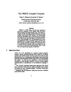
Figure 1. Effects of benchmark and compiler drift, and compiler-only drift on the most significant performance bottlenecks; in descending order of SPEC 95 performance bottleneck significance. row. The last line of the design matrix is a row of -1s. The grayshaded portion of Table 2 illustrates the construction of the PB design matrix for X=8, a design appropriate for investigating 7 (or fewer) parameters. When using foldover, X additional rows are added to the matrix. The signs in each entry of the additional rows are the opposite of the corresponding entries in the original matrix. Table 2 shows the complete PB design matrix with foldover; rows 10 to 17 show the foldover rows. A “+1”, or high value, for a parameter represents a value that is higher than the range of normal values for that parameter while a “-1”, or low value, represents a value that is lower than the range of normal values. Ideally, the high and low values for each parameter should be just outside of the normal range of values. The set of low and high values that we used in this study is similar to those found in [26].

3.1.2 Calculating the significance of performance bottlenecks using the Plackett and Burman design To compute the effect of each parameter, we multiply the execution time by the parameter’s P&B value (+1/-1) for that configuration and sum the resulting products across all configurations. For example, the effect of parameter A is computed as follows: EffectA = (1 * 9) + (-1 * 11) + … + (-1 * 6) + (1 * 4) = -34 Only the magnitude of an effect is important; its sign is essentially meaningless. The effect that a parameter has represents how much of the total variation in the output value is attributable to that parameter. Therefore, if changing the value of a parameter results in large changes in the execution time, then since there is a wide distribution of execution times across a range of processor configurations, there is high variability in the execution time. Consequently, that parameter is a significant performance bottleneck since changing its value results in large changes in the execution time. After simulation, we computed the percentage of the CPI variability across all configurations that can be assigned to each bottleneck, in a manner similar to how ANOVA computes its percentages [15]. By examining the percentage effect that each bottleneck has on the CPI for that suite or benchmark, we can

determine its absolute and relative significance.

3.2 Per-Suite Migration of Performance Bottlenecks Due to Benchmark and Compiler Drift To determine the overall magnitude and scope of the problem, we first compare how the performance bottlenecks migrate as a result of benchmark and compiler drift. More specifically, we compare the performance bottlenecks that are present in the processor when running the SPEC 95 benchmarks that were compiled with a circa 1995 compiler and using 1995 input sets (i.e., B95, C95, I95) against the bottlenecks when running the SPEC 2000 benchmarks that were compiled with a circa 2000 compiler and using 2000 input sets (B00, C00, I00). We first analyze the performance bottlenecks at the suite level, and then, in the following subsection, we examine individual benchmarks in more detail. In Figure 1, the top and bottom lines represent the all-1995 (B95, C95, I95) and the all-2000 design points, respectively, while the middle line represents the effect that compiler drift has on the performance bottlenecks. Therefore, to analyze the effect that the combination of benchmark and compiler drift has on the performance bottlenecks, we need to compare the top and bottom lines. The specific contribution of compiler drift will be analyzed later in this sub-section. Figure 1 shows the percentage effect that each performance bottleneck has on the total variation in the CPI, in terms of the total percentage of variation due to single-factor bottlenecks only, i.e., not due to interaction bottlenecks. (Note: Single-factor bottlenecks account for at least 73.8% of the total variation. In other words, all interactions account for less than 27% of the total variation.) While the results for both suites are shown, the bottlenecks are arranged in descending order of significance for the 1995 bottlenecks for both benchmark suites. This ordering allows for a bottleneck-tobottleneck comparison. Since the percentages are cumulative for each bottleneck, the percentage for the fifth-most important bottleneck represents the total variation in the CPI that is due to the top-five most significant bottlenecks. Although the 1995 curve looks smoother than does the 2000 curve, the uneven nature of the 2000 curve is due only to the ordering of the bottlenecks. An

increasing gap means that a particular bottleneck in SPEC 95 is more significant than in SPEC 2000, while a decreasing gap means that a particular bottleneck is less of a performance bottleneck in SPEC 95. Ovals highlight cases where one bottleneck is significantly more important in one suite than in the other. In this figure, there are two placeholder bottlenecks. Since these placeholders have no physical meaning, their presence in the figure represents the noise threshold. (The noise is the result of using a fractional multifactorial design (i.e., the P&B design) instead of a full one (i.e., ANOVA).) The dotted line corresponds to the location of the more significant of these two placeholders. Any bottlenecks to the right of the dotted line are insignificant since they are below the noise threshold. Figure 1 shows that, of the 43 bottlenecks (41 real bottlenecks and 2 placeholders), only five had a difference in their respective percentages that was greater than 4%. The (SPEC 95 – SPEC 2000) difference is shown in parenthesis for these bottlenecks; a positive number means that that bottleneck is more significant in SPEC 95. Four of the five bottlenecks (the number of reorder buffer (ROB) entries, the L2 cache latency, the L1 I-cache size, and the number of integer ALUs) were more of a problem for SPEC 95 than for SPEC 2000. For the fifth bottleneck, the main memory access time, the opposite is true; this bottleneck is much more of a problem for SPEC 2000 than for SPEC 95. In SPEC 2000, this bottleneck accounts for about five times more variability (4.28% vs. 20.90%). In other words, the main memory access time is a much larger performance bottleneck in SPEC 2000 than in SPEC 95. The big picture from Figure 1 is that two key processor core parameters (the number of ROB entries and the number of integer ALUs) are slightly more important in SPEC 95. However, while the L2 cache latency is a major performance bottleneck in SPEC 95, this performance bottleneck migrates to the main memory level in SPEC 2000. Finally, the L1 I-cache size is more significant in SPEC 95 because its cycle count is not heavily correlated to the main memory latency. Rather, the cycle count is affected by the instruction throughput, which subsequently increases the significance of the L1 I-cache size. From these results, the key conclusion of this sub-section is that benchmark and compiler drift exists between the SPEC 95 and SPEC 2000 benchmarks, when compiled with circa 1995 and 2000 compilers, respectively, since there are non-trivial differences in the most significant performance bottlenecks. To analyze what effect compiler drift may have on the significance of the performance bottlenecks, we compare the middle line with the top line. Since the only difference between these two lines is in what compiler was used, if the two lines exactly track, then compiler drift does not exist. If the two lines diverge, then compiler drift exists. To analyze the contribution that compiler drift makes towards the overall drift, we compare the middle line with the bottom line. Since the difference between the top and bottom lines is the total amount of drift and since the only difference between the top and middle lines is due to the compiler, the distance between the middle and bottom lines represent how much of the total drift is not accounted for by the compiler. Therefore, if the middle and bottom lines exactly track, then benchmark drift does not exist and all of the drift that does exists between the B95, C95, I95 and B00, C00, I00 design points is due only to compiler drift. On the other hand, if the middle line is much closer to the top line, then

compiler drift is less significant than benchmark drift. Of the 25 performance bottlenecks that are above the noise threshold, since the compiler line does not touch the 1995 line at any point, we conclude that compiler drift is a non-trivial phenomenon. Furthermore, with the possible exceptions of the L2 cache latency (Bottleneck #2) and the main memory access latency (Bottleneck #6), since the compiler line tracks the 2000 line fairly well, we also conclude that compiler drift accounts for a significant fraction of the total drift, though not necessarily the majority fraction. (Section 4 quantifies the amount of drift that is due to the benchmark, compiler, and their interaction.) To determine if the compiler drift has a widespread effect, or if it is just limited to the floating-point or integer benchmarks, we examined the corresponding versions of Figure 1 for each benchmark. (Due to space limitations, the figures for all benchmarks are not presented in this section, although the following sub-section presents the figures for mgrid and gcc.) The results show that compiler drift has very little effect for some benchmarks, but it has a large effect for others. For the three integer benchmarks (gcc, perl/perlbmk, and vortex) and for apsi, compiler drift is virtually non-existent as the compiler line almost completely overlays the 1995 line. However, for the three remaining floating-point benchmarks, the compiler line tracks the 2000 line fairly closely, which indicates that compiler drift exists and is very significant.

3.3 Per-Benchmark Migration of Performance Bottlenecks Due to Benchmark and Compiler Drift Figures 2A and 2B show the comparison of the performance bottlenecks for mgrid and gcc, respectively. The organization of each graph is the same as in Figure 1, with the exception that the performance bottlenecks that are less significant than the noise threshold are not shown. We present mgrid since it is representative of the results for the floating-point benchmarks and we present the results for gcc since it clearly shows that most of the drift is due to benchmark drift. As Figure 2A shows, two of the most significant performance bottlenecks in 107.mgrid are the ROB size and the latency of integer multiplies, while less significant performance bottlenecks include the latencies of main memory and L2 cache accesses, both of which are significant bottlenecks of 172.mgrid. Therefore, we conclude that in 107.mgrid, the memory sub-system bottlenecks are relatively minor performance bottlenecks as compared to the instruction execution performance bottlenecks – such as the number of ROB entries, the number of integer ALUs, and the integer multiply latency. By contrast, in 172.mgrid, in addition to the ROB, the most significant performance bottlenecks are the L2 cache size, the memory latency, and the L2 cache latency. Therefore, mgrid clearly shows how the performance bottlenecks move from the processor core and the levels of memory closest to the processor core in the SPEC 95 benchmarks to the memory subsystem or to levels of memory that are further from the processor core in the SPEC 2000 benchmarks. Figure 2B also shows that the performance bottlenecks of gcc also shift towards the levels of memory further away from the processor, albeit in a different way. In contrast to 107.mgrid, the performance bottlenecks of 126.gcc are more heavily concentrated in the processor’s instruction-fetch components (branch predictor, L1 I-cache size, etc.), as opposed to its instruction-execute

100

100

B95, C95, I95 B95, C00, I95 B00, C00, I00

90

80

Percentage of CPI Variation

80

Percentage of CPI Variation

B95, C95, I95 B95, C00, I95 B00, C00, I00

90

70 L2 Cache Latency (-8.55%)

60

Main Memory Access Latency (-16.03%)

50 40 L2 Cache Size (-5.15%)

30

70 Main Memory Access Latency (-3.41%)

60 50

L2 Cache Size (-11.20%)

40 30

Integer Multiply Latency (13.36%)

20

20 Number of ROB Entries (36.02%)

10

L2 Cache Latency (17.56%)

10

L1 I-Cache Size (19.92%)

0

0 0

2

4 6 8 10 12 Bottle ne ck (Decre asing Orde r of B95, C95, I95 Pe rcentage)

14

A. mgrid

0

5

10 15 20 25 Bottleneck (De cre asing Order of B95, C95, I95 Percentage)

30

B. gcc

Figure 2. Effects of benchmark and compiler drift, and compiler-only drift on the most significant performance bottlenecks; in descending order of SPEC 95 performance bottleneck significance. components (number of ALUs and multiply/divide units, instruction latencies, etc.). Therefore, while the performance bottlenecks of 126.gcc also shift from the processor core towards levels of memory further away from the processor, they are on the instruction-fetch side, instead of in the instruction-execute side. Furthermore, since the L2 cache latency is more of a performance bottleneck in 126.gcc, but the L2 cache size is not, this indicates that the L2 cache is able to service most of the memory accesses in 126.gcc. As a result, the L2 cache size is not a performance bottleneck. Finally, of the five remaining benchmarks, drift is a significant problem for swim and applu, due to the increased significance of the memory sub-system parameters. Drift is not as severe a problem for apsi, and is not a problem at all for perl/perlbmk and vortex.

3.4 Potential Simulation Methodology Effects on the Simulation Results and Conclusions 3.4.1 Potential simulation methodology effects on the simulation results and conclusions As described in Section 2.1, since a circa 1995 FORTRAN compiler was not available, we used f2c to translate a benchmark from FORTRAN to C before compiling the resulting C code with a circa 1995 C compiler. Naturally, the key question about this methodology is what effect does f2c have on the results and, more importantly, the overall conclusions? To characterize the effect that f2c has on the simulation results, we compared the performance bottlenecks when a native FORTRAN compiler was used and when using f2c and a C compiler. More specifically, we compiled the three SPECfp 2000 benchmarks (171.swim, 172.mgrid, and 173.applu) where drift was a significant problem (drift was not a significant problem for 301.apsi) with a native circa 2000 FORTRAN compiler and also by using f2c to translate the benchmarks into C first before compiling them with a native circa 2000 C compiler (f2c+cc). Then we applied a P&B design to both sets of binaries to characterize their performance bottlenecks. The results show that for all but one of the bottlenecks, f2c has very little or no effect on their significance. In other words, f2c does not make these bottlenecks significantly more or less important. The one exception is the number of ROB entries; using f2c overestimates its significance, more so for 171.swim and 172.mgrid than for 173.applu. The larger significance of the ROB

size is due to the fact that the f2c+cc generated code contains larger pieces of sequential code, e.g., some code sequences require longer chains of dependent instructions because the compiler has less knowledge about the code and hence can optimize less, which consequently increases the importance of a large ROB, since the ROB is another means of extracting a large amount of parallelism. There are two key conclusions from this sub-section. First, with the exception of overestimating the significance of the number of ROB entries for the floating-point benchmarks, using f2c+cc has very little effect on the results in this paper. And although it does overestimate the significance of the number of ROB entries, it does not change the conclusions in the previous section; namely, that benchmark and compiler drift are significant problems and that the performance bottlenecks migrate from levels of memory closer to the processor to levels that are further away, as a result of drift. Additionally, it does not affect any of the results and conclusions in the rest of this paper.

3.4.2 Potential SimPoint impact It is worth noting that the results in Figures 1, 2A, and 2B, and Table 3 represent a conservative estimate of drift due to the mechanics of how the SimPoint tool chooses simulation points That is, drift is likely to be more severe for the benchmarks with complex phase behavior than the results in the above figures and table would indicate because SimPoint, especially for lower max_K values (we used a max_K of 10), does not choose phase transitions to be simulation points. Using these simulation points may underestimate the effect of the memory access latency [27]. Therefore, benchmarks that spend a significant number of cycles servicing memory accesses, i.e., the SPEC 2000 benchmarks, are likely to have higher-than-expected memory sub-system performance, which partially mitigates the shift of the performance bottlenecks to the memory sub-system that we observed in these experiments.

4. STATISTICALLY-BASED DRIFT MODEL One question from the analysis above is how much of the total drift can be attributed to the benchmark, the compiler, and the interaction of the two? To answer this question we use an ANOVA design [15] to determine what fraction of the CPI variation is due to benchmark drift, compiler drift, and benchmark-plus-compilerinteraction drift when moving between the B95, C95, I95 and B00,

Table 3. Percentage of total drift variation accounted for by each drift component Benchmark

Type

Benchmark Only

Compiler Only

Benchmark + Compiler

swim mgrid applu gcc perlbmk vortex apsi

FP FP FP Int Int Int FP

22.12 18.63 0.91 97.11 78.57 88.64 8.67

75.91 69.67 97.75 0.04 10.10 4.13 14.96

1.97 11.70 1.35 2.85 11.33 7.23 76.38

Int Average FP Average

88.11 12.58

4.76 64.57

7.13 22.85

Suite Average

44.95

38.94

16.11

C00, I00 design points.

4.1 ANOVA Design Methodology For the following four ANOVA testcases: 1) B95/C95, 2) B95/C00, 3) B00/C95, and 4) B00/C00, we simulated a very wide range of configurations (88 in all). Although simulating this many different processor configurations greatly increases the simulation time – as compared to simulating a single processor configuration – there are two key advantages in doing so. First, simulating only a single processor configuration for each testcase may unintentionally skew the results towards one of the three drift components. Obviously, simulating 88 processor configurations minimizes the possibility of inadvertent skew, especially since the different configurations that we simulated corresponded to the “corners” of the design space. Second, and more importantly, by “replicating” the simulation results for each testcase, we can calculate the experimental “error” associated with the variation in CPIs due to different processor configurations. In other words, we can determine how much of the overall variation in the CPIs is due to each factor, i.e., benchmark drift, compiler drift, benchmarkplus-compiler interaction drift, and processor configuration. However, to verify if these 88 atypical processor configurations are either overstating the results or obscuring other important conclusions, we repeated the ANOVA design for 4 realistic processor configurations (base 4-way issue, aggressive 4-way issue, base 8-way issue, and aggressive 8-way issue). Unless otherwise stated, the results for 88 and 4 processor configurations were extremely similar and the conclusions were identical.

4.2 Benchmark and Compiler Drift vs. Processor Configuration Variation The first result that we extract from the 88 processor configuration simulation results is that the processor configuration is responsible for approximately nine times the amount of variation in the CPI as compared to the total of all three drift components. However, it is important to point out that the amount of CPI variation due to different processor configurations is artificially high since the 88 processor configurations correspond to the corners of the design space. For example, one processor configuration has an 8-entry ROB, a single integer ALU, a 2-entry LSQ, and a 2KB, directmapped L1 D-cache while another processor configuration has a 64-entry ROB, four integer ALUs, a 64-entry LSQ, and 128KB, 8way L1 D-cache. Consequently, one can, to a certain degree,

expect large variations in the CPI solely due to the processor configuration. For the 4 realistic processor configurations, the results were extremely similar to the results of the 88 configurations for some benchmarks. However, for other benchmarks, the percentage of the CPI variation that is a result of drift is almost the same as the percentage of the CPI variation that is accounted for by the processor configuration. For example, for perl/perlbmk, benchmark drift accounts for 45.7% of the total CPI variation while changing the processor configuration accounts for 48.8%. This particular result shows that benchmark drift can have as much of an impact on the CPI as changing the processor configuration from a simple 4-way issue processor to an aggressive 8-way issue one. Or, in other words, benchmark drift has as significant an impact on the execution time of benchmarks such as perl/perlbmk as radically changing the processor configuration. Our conclusion from this sub-section is that the processor configuration generally has more impact on the variation in the CPIs than benchmark and compiler drift does. For some benchmarks, however, drift and processor configuration account for similar percentages of the CPI variation.

4.3 Statistically-Based Drift Model Results Table 3 shows the percentage of the CPI variation that is accounted for by each of the three drift components, after removing the variation due to the 88 processor configurations. The results for the 4 realistic processor configurations were extremely similar. Across all seven benchmarks, these results show that benchmark drift is only slightly more significant than compiler drift. However, for the integer benchmarks taken as a group, benchmark drift accounts for nearly all of the CPI variation that is attributable to drift. The opposite conclusion is true for the floating-point benchmarks, although the difference is not quite as dramatic. In these benchmarks, compiler drift is the dominant reason for the variation in CPI, although the benchmark-plus-compiler interaction accounts for a significant percentage of the total CPI variation. Based on these results, we conclude that benchmark drift is at least 15% ((44.95-38.94) / 38.94) more significant than compiler drift. Furthermore, both drift components are at least twice as significant as benchmark-plus-compiler-interaction drift.

5. IMPACT OF DRIFT ON THE OPTIMAL PROCESSOR DESIGN CONFIGURATION The two key conclusions from the previous sections are that benchmark and compiler drift exist and that the performance bottlenecks migrate towards levels of memory further away from the processor. While these are important conclusions, the key question is what, if any, differences in the optimal processor configuration result from benchmark and compiler drift and the subsequent migration of the performance bottlenecks? And, if there is a difference, what performance impact does it make? To answer these questions, this section studies how drift affects the optimal processor configuration. Specifically, the question we address is how much of the performance potential is lost due to drift, and for what reasons? With this goal in mind, we optimize one processor configuration for the B95, C95, I95 (the “SPEC 95 optimized processor”) design point and another processor for B00, C00, I00 (the “SPEC 2000 optimized processor”) design point. The former design point is what an architect might start at when designing a new processor in 1995, while the second design point would

1. 2.

3.

Assign i = 0 and choose an initial configuration as the current optimal configuration Ci,0 For each architectural parameter j, with 0 < j ≤ n, a. Determine the optimal value for parameter j while keeping the other parameters at their current optimal configuration Ci,j-1 values b. Update the current optimal configuration Ci,j with the latest optimal configuration for the given parameter If the current optimal configuration Ci,n equals the previously obtained optimal configuration Ci-1,n, stop and report Ci,n as the optimal configuration; otherwise, increment i and go to step 2.

Figure 3. One-Parameter-At-A-Time Algorithm to Find the Optimal Processor Configuration correspond to the potential design point when the processor is released in 2000. If there is a considerable difference in the two optimal processor configurations, we can conclude that drift has a significant impact on processor design, and then we can determine how drift affects the optimal configuration. We can also quantify the lost performance potential by comparing the performance of SPEC 2000 when executed on the SPEC 95 optimized processor compared to the performance of SPEC 2000 when run on the SPEC 2000 optimized processor. Before presenting the results from this study, we first discuss our optimal processor design search algorithm and our optimization criterion.

5.1 Optimal Design Point Search Algorithm To determine the optimal processor configuration, we used the one-parameter-at-a-time optimization algorithm. As its name implies, in this algorithm, only one parameter is optimized (i.e., varied) at a time. After optimizing each parameter, the value of that parameter is set to the value that yields the optimal result and then the next parameter is optimized. For example, assume that we are trying to optimize parameters x, y, and z that start with an initial configuration of x3, y1, and z1. If x is the first parameter to optimize, we measure the optimality of the following processor configurations {x1, y1, z1}, {x2, y1, z1}, … , {xn-1, y1, z1}, {xn, y1, z1}, where n is the number of values parameter x can be set to. If configuration {x2, y1, z1} is optimal, we change the value of x from x3 to x2, and then optimize parameter y across its range of values. After optimizing all three parameters, we check to see if there was any change in the optimal configuration since the last time parameter z was optimized. If not, then the last configuration is the

optimal one. If so, then we re-optimize all three parameters repeatedly until the configuration does not change for a single iteration of all three. The specifics of the algorithm are shown in Figure 3. Although this search algorithm optimizes only one parameter-at-atime, by repeatedly optimizing all parameters until the processor configuration “converges”, this optimization algorithm minimizes the likelihood of getting trapped in local minimum. For these simulations, several iterations were required until the configuration stabilized. Additionally, to further minimize the likelihood of getting trapped in a local minimum, we optimize the parameters in descending order of significance (i.e., the most significant parameter is optimized first, then the second most significant parameter is optimized next, and so on). Finally, we chose this algorithm based on our observation that processor designers use this type of algorithm due to its fast search time. Of the 41 performance bottlenecks, the ten most significant ones for B95, C95, I95 were also in the list of the ten most significant ones for B00, C00, I00, but just in a different order. Since the11th, 12th, etc. most significant bottlenecks from each design point were different, we were unable to find another set of bottlenecks to optimize over such that we would be optimizing over the Top N bottlenecks from both design points, and that did not require optimizing over an intractable number (i.e., all 41) of bottlenecks. Therefore, we optimized over just these ten bottlenecks, which are listed in Table 4 along with their range of candidate values. The range of possible values was based on current processors. Finally, the third column shows the initial configuration of both processors, which was randomly chosen. Although the cache access latencies are not listed, each of these latencies were based on the current size, associativity, and block size of each cache. For the L1 caches, the latencies ranged from 1 to 4 cycles, while for the L2 cache, the latency ranged from 7 to 12 cycles. To reduce the simulation time, we fixed the number of load-store queue (LSQ) entries to always be half of the number of ROB entries. Therefore, optimizing for the number of ROB entries really optimized both the number of ROB entries and the number of LSQ entries. To reduce the simulation time further, since several serialized iterations were required before the configuration stabilized, we used only a single input set for 126.gcc (cp-decl), 134.perl (scrabbl), 176.gcc (expr), 253.perlbmk (splitmail 957), and 255.vortex (lendian3). We chose these input sets since their vector of CPIs from the P&B design simulations was closest to the centroid of the space for that benchmark.

Table 4. Performance bottlenecks to optimize, possible values, and initial configuration Bottleneck Number of Reorder Buffer (ROB) Entries L2 Cache Associativity L2 Cache Size L1 I-Cache Size Branch Predictor Entries Number of Integer ALUs L1 D-Cache Size L1 D-Cache Associativity L1 I-Cache Block Size in Bytes Number of Load-Store Queue Entries

Possible Values 32, 64, 96, 128, 160 2-Way, 4-Way, 8-Way 512KB, 1024KB, 2048KB, 4096KB 32KB, 64KB, 128KB 1024, 2048, 4096 2, 3, 4 16KB, 32KB, 64KB 2-Way, 4-Way, 8-Way 32, 64 0.5 * Number of ROB Entries

Initial Configuration 32 2-Way 2048KB 32KB 4096 3 16KB 2-Way 32 16

Table 5. Optimal processor configurations for SPEC 95 and SPEC 2000 derived processors, arranged in decreasing order of SPEC 2000 parameter significance Bottleneck Number of Reorder Buffer (ROB) Entries L2 Cache Associativity L2 Cache Size L1 I-Cache Size Branch Predictor Entries Number of Integer ALUs L1 D-Cache Size L1 D-Cache Associativity L1 I-Cache Block Size in Bytes Number of Load-Store Queue Entries

SPEC 95 96 4-Way 2048KB 32KB 4096 4 16KB 4-Way 64 48

SPEC 2000 160 4-Way 1024KB 32KB 4096 4 16KB 4-Way 64 80

Comment SPEC 2000 optimized processor opts for a much larger ROB SPEC 2000 optimized processor opts for a smaller L2 cache

SPEC 2000 optimized processor opts for a much larger LSQ

Table 6. Percent difference in CPI and EDP between the SPEC 95 and SPEC 2000 optimized processors for two SPEC 2000 processor L2 cache sizes (1024KB (optimal) and 2048KB); Percent difference = (SPEC 95 – SPEC 2000) / SPEC 2000 Benchmark 171.swim 172.mgrid 173.applu 176.gcc 253.perlbmk 255.vortex 301.apsi Average

1024 KB L2 Cache (Optimal) Percent CPI Difference Percent EDP Difference 52.41 74.24 14.56 12.49 31.44 36.90 -3.73 -16.04 -1.78 -13.41 -0.68 -10.92 12.16 6.62 20.84 18.55

Consequently, using a sub-set of the input sets should have very little effect on the final optimized configuration. Without an associated “cost” to each of the bottlenecks listed in Table 4, the optimization algorithm will predictably choose the largest value of each parameter in an effort to decrease the execution time. Therefore, in this paper, we define the optimal processor configuration to be the one with the minimum energydelay product (EDP), where EDP = EPI * CPI (EPI = Energy per Instruction and CPI = Cycles per Instruction). The energy-delay product is a commonly used metric that quantifies the energyefficiency of general-purpose microprocessors [4]. While there are alternative optimization cost functions in commercial processor design, these cost functions are very complex since they utilize a wide range of optimization criteria and design constraints, such as CPI, cycle time, chip area, power budget, heat transfer, power density, reliability, etc. In this paper, however, we use the simple and easy-to-understand EDP optimization criterion.

5.2 Optimized Processor Configuration Results and Discussion Table 5 presents the optimized processor configuration for each benchmark suite. The first column lists the performance bottlenecks that we optimized for. The second and third columns list the final optimal processor configuration when optimizing for the SPEC 95 and SPEC 2000 benchmarks, respectively. The fourth column summarizes the difference, for each parameter, between the two processors. The comment column in Table 5 shows that there are two key differences between the SPEC 95 and SPEC 2000 optimized processors. First, the configuration of the SPEC 2000 optimized processor uses a much larger ROB than the SPEC 95 optimized

2048KB L2 Cache Percent CPI Difference Percent EDP Difference 53.02 67.93 16.28 10.28 32.21 33.04 0.86 -12.93 1.96 -10.90 4.27 -7.29 11.46 2.37 22.73 17.19

processor, even though using f2c to compile the SPECfp 95 benchmarks may result in an artificially large ROB. On the other hand, the SPEC 2000 optimized processor selects the largest number of ROB entries possible. While this result may seem surprising from an EDP point-of-view (increasing the number of ROB and LSQ entries is very expensive from an energy point-ofview), there are several reasons that explain this outcome. First and foremost, the number of ROB entries is the most significant bottleneck in SPEC 2000. As a result, it is not that surprising that the SPEC 2000 optimized processor would opt for a large ROB, even given the high energy cost. Second, a processor with a larger ROB can hide the L2 cache misses by exploiting parallelism. Third, in addition to buffering a larger number of loads and stores, an 80-entry LSQ – at least in SimpleScalar – essentially functions as a de facto L0 D-cache, which increases the chances for store-forwarding, reduces the number of L1 D-cache cast-outs, and slightly decreases the number of L1 D-cache and L2 cache accesses (by satisfying load accesses via store forwarding). Therefore, a larger ROB and LSQ is more efficient from an EDP point-of-view due to its ability to hide the memory sub-system access latency and since the LSQ functions as a low-latency, fully-associative L0 Dcache. The SPEC 2000 optimized processor also opts for a smaller L2 cache (1024KB vs. 2048KB). However, as the results in Section 3 showed, since the memory latency is more significant of a performance bottleneck in SPEC 2000, it is surprising to see that the L2 cache of the SPEC 2000 optimized processor is smaller than that of the SPEC 95 optimized processor’s. However, there are three reasons for this difference. First, the larger LSQ reduces the number of L2 cache accesses (by using store forwarding to decrease the number of L1 D-cache accesses, which, in turn, reduces the number of L2 cache accesses), which decreases the

significance of the L2 cache as a performance bottleneck. Second, although a larger L2 cache increases the hit rate, the associated trade-off is that the cache access latency increases by a cycle when the L2 cache doubles in size. Third, although the CPI for a processor with a 2048KB L2 cache is 1.54% lower than a processor with a 1024KB L2 cache, it consumes 2.74% more energy, which results in a sub-optimal EDP. Nevertheless, since the difference in the EDPs between the two L2 sizes was only 1.15%, the final L2 cache size for the SPEC 2000 optimized processor was very close to being a toss-up.

5.3 Effect of Different Optimized Configurations on the Performance and Energy-Delay Product Although the results from Section 3 and the previous sub-section concluded benchmark and compiler drift exist and is a significant enough of a problem to alter the optimized processor configuration, the singular outstanding question is how much difference – in terms of the CPI and EDP – can drift actually have? To answer this question, we compare the performance (CPI) and the EDP of the SPEC 95 and SPEC 2000 optimized processors when both processors run the SPEC 2000 benchmarks, which is the situation that a processor designer would have faced when originally designing the processor in 1995. Table 6 presents the CPI and EDP results of this comparison. The first column lists the benchmarks, while the second/fourth and third/fifth columns list the difference in the CPIs and EDPs, respectively, when the SPEC 2000 optimized processor is the baseline ((SPEC 95 – SPEC 2000) / SPEC 2000)). Therefore, larger, positive numbers means that the SPEC 2000 optimized processor achieves a lower CPI (i.e., higher performance) or a lower EDP (i.e., better energy efficiency). Overall, the results show that the CPI of the SPEC 2000 optimized processor with a 1024KB L2 cache is 20.84% better than the CPI of the SPEC 95 optimized processor, while the EDP is 18.55% better. Consequently, we conclude that benchmark and compiler drift can result in large performance and EDP differences between the optimized processor configurations. The large difference in the CPIs and EDPs are strictly due to the floating-point benchmarks, which is not surprising given that the most significant performance bottleneck in the SPECfp 2000 benchmarks is the number of ROB entries and that the SPEC 2000 optimized processor has an additional 64 ROB and 32 LSQ entries. On the other hand, since the significance of the L2 cache size as a performance bottleneck is much lower than the significance of the number of ROB entries, increasing the L2 cache size (which also incurs an increase in the L2 cache access latency) does not significantly improve the CPI. For the integer benchmarks, since the ROB is not one of the most significant performance bottlenecks, using a larger ROB does not result in significant performance improvements, but does significantly increase the EDP. On the other hand, since the LSQ is about as significant a performance bottleneck as the L2 cache size, the larger LSQ helps palliate the effect of the L2 cache size as a performance bottleneck. Lastly, although the CPI decreases by 1.54% as a result of the larger L2 cache size, the associated EPI increase of 2.74% more than offsets the CPI gain from an EDP point-of-view, which makes this configuration less than optimal. The key conclusion from this section is that using older benchmarks and compilers for processor design can result in processor configurations that are significantly different than when the latest benchmarks and compilers are used, and that the

performance and energy efficiency of the former configurations can be dramatically lower – in this case, a CPI and EDP that are 20.84% and 18.55% higher, respectively. The combination of this conclusion and one from the previous section – that drift can have as significant an impact on the CPI as radically changing the processor configuration – show that processor designers and computer architecture researchers need to be conscious of benchmark and compiler drift in their studies since it can significantly distort their simulation results. Furthermore, these conclusions should also encourage architects to continually examine and characterize benchmark and compiler trends.

6. RECOMMENDATIONS TO MINIMIZE AND ACCOUNT FOR THE EFFECTS OF DRIFT The results in Section 4 showed that benchmark and compiler drift can have as much impact on the CPI as radical changes in the processor configuration, while the results in Section 5 showed that drift can change the optimized processor configuration enough to result in performance that is significantly sub-optimal. As a result, since this phenomenon has the potential to not only gravely affect the performance of commercial processors, but to influence, subtly or otherwise, the directions of computer architecture research, it is very important for computer architects to account for and/or minimize the effects of drift. Accordingly, we make the following recommendations: 1.

Benchmark suites and compilers, such as SPEC and gcc, respectively, should be updated more frequently.

2.

Parameterizable benchmarks, such as those described in [1, 2, 20] should be used to project the potential effects of benchmark and compiler drift.

Since the characteristics of future benchmarks and compilers change over time, updating both more frequently minimizes the “abruptness” of the changes in their characteristics. If computer architects follow these recommendations, although there will be less drift between successive versions of a benchmark suite or compiler, the total amount of drift over the same amount of time (i.e., without more frequent updates) will still be the same. As their name implies, with parameterizable benchmarks, the characteristics of the benchmark can be easily adjusted by changing the value of a parameter. By using a range of parameter values, computer architects may be able to mimic the characteristics of future benchmarks, which may allow them to properly compensate for the effects of drift. In other words, computer architects can use parameterizable benchmarks to perform “what-if” experiments to help optimize the processor’s configuration to account for future drift. Finally, it is important to note that while these recommendations minimize the effects of drift, they do not eliminate them as benchmark and compiler drift cannot be eliminated.

7. RELATED WORK Phansalkar et al. [16] studied how the SPEC CPU benchmarks (1989, 1992, 1995, and 2000) change over time. They looked at microarchitecture-independent characteristics in order to identify changes in the workload and used principal component analysis to characterize and compare the benchmark suites, but did not

evaluate the impact of drift on processor design. Their results showed that other than dramatic increases in the dynamic instruction count and increasingly poor temporal data locality, fundamental program characteristics such as branch and ILP characteristics are generally static. Our paper also studies the effect that workload changes have on processor’s performance, adds compiler drift as a factor, and constructs a drift model. Vandierendonck and De Bosschere compare the data memory behavior of SPEC 95 and SPEC 2000 in [22]. Their results show that some SPEC 95 benchmarks have behavior that is very different than the behavior of the other benchmarks. Furthermore, their results show that this behavior can be easily improved, which SPEC addressed for selected benchmarks in the SPEC 2000 suite. Calder et al. [6] compared the characteristics of C and C++ programs including: function and basic block sizes, instructions between conditional branches, call stack depth, use of indirect function calls and memory operations, and measurements of cache locality. The C programs that they examined included the SPECint 92 suite, while the remaining C and all of the C++ programs were gathered from a variety of sources. Consequently, their results did not explicitly examine benchmark drift. Standardized benchmark suites, such as the various SPEC benchmark suites [21], are updated regularly. A benchmark may be modified or removed when it is no longer representative or has reproducible results, or if compiler optimizations drastically reduce its execution time. Examples of the latter include matrix300 from SPEC 89 [12] and eqntott from SPEC 92 [24]. In the case of sc, system libraries had too large an impact on the running time of the benchmark [7]. As a result, all of these programs were removed from subsequent SPEC benchmark suites. Another compelling reason to update benchmarks is benchmark drift. SPEC recognizes that they have to “keep pace with the breakneck speed of technological innovation” [13] and intentionally selected SPEC 2000 benchmarks such that they consume much more memory than SPEC 95 [14]. Given the prevalent use of benchmarks in computer architecture, one would expect that many quantitative metrics or methods have been developed to evaluate and improve the appropriateness of a benchmark suite. However, few efforts have been directed in this area. Dujmovic et al. [9] developed metrics to estimate the size and redundancy of a benchmark suite. Using these metrics, they showed that the SPEC benchmark suite has increased in size (i.e., more differences between processors can be detected) and that redundancy decreased between the SPEC 89 and SPEC 95 versions. Eeckhout et al. [10] developed a method to gauge benchmark similarity (and thus redundancy). By applying cluster analysis techniques on workload characteristics, identifying benchmarks that are similar is relatively easy.

8. CONCLUSION As the time required to design a processor continues to increase, it is increasingly likely that different generations of a benchmark suite and different versions of the same compiler will be used in the design process. If the characteristics of the successor suite or compiler are significantly different than those of their respective predecessors, then the design decisions that the processor architects make early in the design cycle may be sub-optimal when the performance is measured using the most current suite available after the processor is fabricated and the benchmarks are compiled with the latest compiler. We coin the terms benchmark drift and compiler drift to refer to the phenomenon of time-varying

benchmark and compiler characteristics, respectively. Our results show that both benchmark and compiler drift exist and are potentially significant problems. Furthermore, the most significant performance bottlenecks for the SPEC 95 benchmarks are in the processor core and in the levels of memory closest to the processor, while these bottlenecks migrate to levels of memory further away from the processor core for the SPEC 2000 benchmarks. Our results also show that benchmark drift is at least 15% more significant than compiler drift, while both components are at least twice as significant as the drift due to the interaction of the benchmark and compiler. Furthermore, the results show that for some benchmarks, perl/perlbmk in particular, drift has as significant effect on the CPI as does dramatically changing the processor configuration. After using the one-parameter-at-a-time optimization algorithm and the energy-delay product (EDP) as the optimization criterion to find the optimal processor configuration, the SPEC 2000 optimized processor opts for a much larger reorder buffer (160 entries vs. 96 entries), but selects an L2 cache that is half the capacity as the SPEC 95 optimized processor’s L2 cache. These differences in the optimal processor configurations led to very large differences in the CPI and EDP. More specifically, the CPI for the SPEC 2000 optimized processor is 20.84% lower than in the SPEC 95 optimized processor, while the EDP is 18.55% lower. Finally, to help computer architects compensate for the effects of drift for research and design, we recommend that computer architects: 1) Update benchmark suites and compilers more frequently and 2) Use parameterizable benchmarks to (potentially) project the characteristics of future benchmarks and compilers. In summary, the two key conclusions from this paper are that benchmark and compiler drift exist and that drift can significantly affect processor design and its subsequent performance. Or, in other words, the exigency of benchmark and compiler drift is that tomorrow’s processors are being designed using yesterday’s benchmarks and compilers, with potentially serious performance degradation and energy implications due to significantly different characteristics.

9. Acknowledgements This work was supported in part by IBM, Intel, the University of Minnesota Digital Technology Center, the Minnesota Supercomputing Institute, Ghent University, and the European HiPEAC network of excellence. Hans Vandierendonck and Lieven Eeckhout are Postdoctoral Fellows of the Fund for Scientific Research – Flanders (Belgium) (F.W.O. Vlaanderen).

10. REFERENCES [1] Bell Jr., R. and John, L., “The Case for Automatic Synthesis of Miniature Benchmarks,” In Proceedings of the Workshop on Modeling, Benchmarking, and Simulation (MoBS ’05) (Madison, WI, USA, June 4-8, 2005), 88-97. [2] Bell Jr., R. and John, L., “Improved Automatic Testcase Synthesis for Performance Model Validation,” In Proceedings of the International Conference on Supercomputing (ICS ’05) (Cambridge, MA, USA, June 20-22, 2005), 111-120. [3] Brooks, D., Tiwari, V., and Martonosi, M., “Wattch: A Framework for Architectural-Level Power Analysis and Optimizations,” In Proceedings of the International Symposium on Computer Architecture (ISCA ’00)

(Vancouver, Canada, June 10-14, 2000), 83-94. [4] Brooks, D., Bose, P., Schuster, S., Jacobson, H., Kudva, P., Buyuktosunoglu, A., Wellman, J., Zyuban, V., Gupta, M., and Cook, P., “Power-Aware Microarchitecture: Design and Modeling Challenges for Next-Generation Microprocessors,” IEEE Micro, 20, 6, (Nov./Dec. 2000), 26-44. [5] Burger, D. and Austin, T. “The SimpleScalar Tool Set, Version 2.0,” ACM Computer Architecture News, (June 1997), 13-25. [6] Calder, B., Grunwald, D., and Zorn, B., “Quantifying Behavioral Differences Between C and C++ Programs,” Journal of Programming Languages, 2, 4, (1994), 313-351. [7] Carlton, A., “Lessons Learned from 072.sc”, SPEC Newsletter, (Mar. 1995). [8] Choi, Y., Knies, A., Gerke, L., and Ngai, T., “The Impact of If-Conversion on Branch Prediction and Program Execution on the Intel Itanium Processor,” In Proceedings of the International Symposium on Microarchitecture (Micro ’01) (Austin, TX, December 2-5, 2001), 182-191. [9] Dujmovic, J. and Dujmovic, I., “Evolution and Evaluation of SPEC Benchmarks,” ACM SIGMETRICS Performance Evaluation Review, 26, 3, (Dec. 1998), 2-9. [10] Eeckhout, L., Vandierendonck, H., and De Bosschere, K. , “Workload Design: Selecting Representative Program-Input Pairs,” In Proceedings of the International Conference on Parallel Architectures and Compilation Techniques (PACT ’02) (Charlottesville, VA, USA, September 22-25, 2002), 8394. [11] Hamerly, G., Perelman, E., and Calder, B., “How to Use SimPoint to Pick Simulation Points,” ACM SIGMETRICS Performance Evaluation Review, 31, 4, (Mar. 2004), 25-30. [12] Hennessy, J. and Patterson, D., “Computer architecture: A Quantitative Approach,” Morgan-Kauffman, San Francisco, CA, 2003. [13] Henning, J., “SPEC CPU2000: Measuring CPU Performance in the New Millennium,” IEEE Computer, 33, 7, (Jul.. 2000), 28-35. [14] Henning, J., “SPEC CPU2000 Memory Footprint,” http://www.spec.org/cpu2000/analysis/memory [15] Lilja, D., “Measuring Computer Performance,” Cambridge University Press, New York, NY, 2000.

[16] Phansalkar, A., Joshi, A., Eeckhout, L., and John, L., “Measuring Program Similarity: Experiments with SPEC CPU Benchmark Suites,” Proceedings of the International Symposium on Performance Analysis of Systems and Software (ISPASS ’05) (Austin, TX, March 20-22, 2005), 10-20. [17] Plackett, R. and Burman, J. ”The Design of Optimum Multifactorial Experiments,” Biometrika, 33, 4, (June 1946), 305-325. [18] Sherwood, T., Perelman, E., Hamerly, G., and Calder, B., “Automatically Characterizing Large Scale Program Behavior,” In Proceedings of the International Conference on Architectural Support for Programming Languages and Operating Systems (ASPLOS ’02) (San Jose, CA, USA, October 5-9, 2002), 45-57. [19] http://www.cs.ucsd.edu/~calder/simpoint [20] Skadron, K., Martonosi, M., August, D., Hill, M., Lilja, D., and Pai, V., “Challenges in Computer Architecture Evaluation,” IEEE Computer, 36, 8, (Aug. 2003), 30-36. [21] http://www.spec.org [22] Vandierendonck, H. and De Bosschere, K., “Eccentric and Fragile Benchmarks,” In Proceedings of the International Symposium on Performance Analysis of Systems and Software (ISPASS ’04) (Austin, TX, March 10-12, 2004), 2-11. [23] http://www.eecs.umich.edu/~chriswea/benchmarks/SPEC 2000.html [24] Weicker, R., “An Example of Benchmark Obsolescence: 023.eqntott,” SPEC Newsletter, (Dec. 1995). [25] Wulf, W. and McKee, S., “Hitting the Memory Wall: Implications of the Obvious,” ACM Computer Architecture News, 23, 1, (Mar. 1995), 20-24. [26] Yi, J., Lilja, D., and Hawkins, D., “A Statistically Rigorous Approach for Improving Simulation Methodology,” In Proceedings of the International Symposium on HighPerformance Computer Architecture (HPCA ’03) (Anaheim, CA, USA, February 8-12, 2003), 281-291. [27] Yi, J., Kodakara, S., Sendag, R., Lilja, D., and Hawkins, D., “Characterizing and Comparing Prevailing Simulation Techniques,” In Proceedings of the International Symposium on High-Performance Computer Architecture (HPCA ’05) (San Francisco, CA, USA, February 12-16, 2005), 266-277.