Below, we provide details of our generative model for finding. PTM groups and derivation of our inference algorithm using the. EM algorithm. This is additional to ...
PTMClust: Supplementary Information
THE EXPECTATION-MAXIMIZATION ALGORITHM In this section we provide a brief summary of the ExpectationMaximization (EM) algorithm. For details and theoretical understanding of the EM algorithm we recommend readers to refer to the following references (Dempster et al. (1977); McLachlan and Krishnan (1997)). The EM algorithm is an elegant and powerful method for finding the maximum likelihood of models with hidden variables. The key concept in the EM algorithm is that it iterates between the Estep and M-step until convergence. In the E-step, the algorithm estimates the posterior distribution of the hidden variables Q (also refer to as the responsibility) given the observed data and the current parameter settings; and in the M-step the algorithm calculates the ML parameter settings with Q fixed. At the end of each iteration the lower bound on the likelihood is optimized for the given parameter setting (M-step) and the likelihood is set to that bound (E-step), which guarantees an increase in the likelihood and convergence to a local maximum, or global maximum if the likelihood function is unimodal. Formally, for N input data points at iteration t, given the current parameter settings θt−1 calculated in the previous iteration, the Estep estimates the responsibility Q for the nth input data point as Qnhn = P (hn |vn , θ
t−1
P (hn , vn |θt−1 ) )= P . t−1 ) hn P (hn , vn |θ
Mixing coefficient
(1)
where hn are the hidden (latent) variables, vn are the observed variables and θt−1 are the model parameters for iteration t − 1. In the M-step, while fixing Qnhn , the parameters are estimated by maximizing the expected log likelihood "N # X ln P (hn , vn |θ) , (2) θt = arg max Ehn θ
= �N P
arg max θ
n N X X n
observation is generated. For a given PTM type (PTM group), the observed modification mass is assumed to be a noisy version of the expected (mean) modification mass, and the modified amino acid is chosen from a distribution over amino acids that may be modified in that type. For example, modifications occur primarily on serine (S) and threonine (T) for phosphorylation. For a given peptide, the true modification position is assumed to be chosen uniformly among occurrences of that amino acid in the peptide. Finally, the observed modification position is assumed to be a noisy version of the true position. Below, we described the components of our model: the probability of choosing each PTM type, the probability of choosing each amino acid to be the modified amino acid given the PTM type, the probability of the true modification position given the modified amino acid, and the uncertainty in the observed modification mass and modification position. We then introduced an algorithm for learning the model parameters and inferring the hidden (latent) variables from the input data. Once a model is learned, we can refine the modification for each input peptide sequence by inferring its most likely PTM group, true modification mass and true modification position.
Qnhn ln P (hn , vn |θ),
Modification mass mean Modification mass variance
cn
Observed modification Mass
PTM groups
Amino acid modified
mn Peptide sequence
N Prob. of amino acid modified
an
Sn
Correct modification position
zn
Observed modification position
xn
hn
� ln P (hn , vn |θ) is the expectation of the log
PTMCLUST - A GENERATIVE MODEL FOR FINDING PTM GROUPS
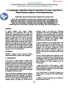
Fig. 1. A Bayesian network describing our generative model, using plate notation. The shaded nodes represent observed variables, the unshaded nodes represent latent variables and the variables outside the plate are model parameters. The model describes how the observed modification mass and modification position are generated. Given the type of PTM (PTM group), we can generate the observed modification mass as a noisy version of the modification mass mean, and select an amino acid to have the modification as the modified amino acid. Given the peptide sequence, we can choose a position along it that matches the modified amino acid as the ’true’ modification position. We can generate the observed modification position as a noisy version of the ’true’ modification position. The plate notation indicates there are N copies of the model, one for each input data. This is the same figure presented in the main manuscript.
Below, we provide details of our generative model for finding PTM groups and derivation of our inference algorithm using the EM algorithm. This is additional to the description provided in the Method section of the main manuscript. To make it easy for the reader to follow we have repeated related information from the Method section in the main manuscript. By accounting for combinatorial interactions between hidden variables that play a role in the protein modification process, our generative probability model aims to describe how each PTM
The structural relationship between the variables described below is indicated by the Bayesian network from Fig. 1. It describes the model for one input and is repeated for N inputs, as indicated by the plate notation (box in the figure). In our model, each input peptide sequence Sn , indexed by n ∈ {1, ..., N } where N is the number of peptides in the dataset, has a corresponding discrete peptide length Ln , observed modification position xn ∈ {1, ..., Ln } and observed modification mass mn .
where Ehn
n
likelihood respect to the hidden variables hn for the nth data point. The EM algorithm can be altered to calculate MAP instead of ML parameter settings by switching the ML estimation in the M-step with MAP estimation. As an example, the EM algorithm is applied to learn our proposed algorithm PTMClust (see below).
1
Chung et al
Sn (j) is the amino acid in position j of the input sequence n. The total number of values Sn (j) can take on is A = 24, which includes the 20 naturally occurring amino acids and four special characters indicating the beginning and end of proteins and peptides. The latent variable cn ∈ [1, .., K] denotes the unknown PTM group for peptide sequence n, where K is the number of PTM groups and will be adjusted depending on the desired false detection rate, as described later. The prior probability (mixing coefficient) for each PTM group is given as P (cn = k) = αk , (3) where it satisfies the constraints αk ≥ 0 and
K P
chosen because it is the minimum number of entries per group needed to calculate a reasonable mean and variance, provides a large enough dataset (1206) to estimate the likelihood function, and acts as a crude filter for false modified peptides. The frequency of peptides for each group size, shown in Supplementary Fig. 1, exhibits a heavy-tail curve where majority of modified peptides have low counts. More than 48% of the entries have a group of size exactly three. The resulting likelihood distribution is shown in Fig. 2.
αk = 1, and is
0.5
k=1
inferred from the data (see below for detail). The probability that the PTM occurs on amino acid i ∈ {1, ..., A}, given that the PTM group is k, is (4)
where the latent variable an denotes the true (unobserved) modified A P amino acid and the β’s satisfy the constraints βki ≥ 0 and βki =
Likelihood
P (an = i|cn = k) = βki ,
0.4
0.3
0.2
i=1
1, and is inferred from the data (see below for detail). Given the peptide sequence Sn and the modified amino acid an , each occurrence of that amino acid in the peptide sequence has equal probability of being the true (unobserved) modification position zn . For completeness, our probabilistic model considers the likelihood of cases where an amino acid does not occur in Sn . To do so, we allowed for the event that the true PTM occurs outside of the given peptide sequence 1 , indicated by zn = 0, so that zn ∈ {0, ..., Ln }. All other positions in the peptide sequence have zero probability of being the true modification position. This can be written as
P (zn = j|an = i, Sn ) =
1 δni +1 1 δni +1
0
if Sn (j) = i, j ≥ 1, if j = 0, otherwise,
(5)
where δni denotes the number of times amino acid i occurs in sequence n. We modeled the modification position error (xn − zn ) between the observed modification position xn and the true modification position zn with a discrete probability distribution, given as φ(xn − j) if j > 0, φ(Ln ) if j = 0, P (xn |zn = j) = (6) 0 otherwise, where the likelihood function φ accounts for the modification position error. This likelihood function is shared across all PTM groups and is inferred from our empirical observation of the yeast PTM dataset as follows (see Results section in the main manuscript for description of the dataset). We grouped the entries in the dataset by their peptide sequence and modification mass, allowing for mass difference of +/- 2 Da and removing groups with less than three entries. Then, we determined the average modification position for each group (rounded to the nearest position) and computed a histogram of the modification position error. Three entries was 1
zn = 0 is needed to avoid numerical issues since our algorithm considers each amino acid as a possible modification target.
2
0.1
0
−7 −6 −5 −4 −3 −2 −1 0 1 2 3 4 5 6 7 Modification Position Error (No. of Residues)
Fig. 2. Distribution of Modification Position Error used by PTMClust. This empirical distribution was derived using yeast PTM data (Krogan et al. (2006)) analyzes with SIMS (Liu et al. (2008)). A positive (negative) modification position error indicates the observed modification position is towards the C-terminus (N-terminus) of the expected modification position. This is the same figure presented in the main manuscript.
Lastly, we accounted for the variation (noise) in the estimated modification mass by assuming the observed modification mass for each PTM group is normally distributed around the true modification mass, given as 1 exp P (mn |cn = k) = √ 2πΣk
�
−(mn − µk )2 2Σk
� ,
(7)
where µk and Σk are the modification mass mean and variance for the kth PTM group, and are inferred from the data (see below for detail). Combining the structure of the Bayesian network and the conditional distributions described above, we can write the joint distribution as P (c, a, z, x, m|S, θ) = N Q
� P (cn |θ)P (mn |cn , θ)P (an |cn , θ)P (zn |an , Sn , θ)P (xn |zn , θ) ,
n=1
(8) where θ represents the model parameters (αk , βki , µk and Σk ). The input data are noisy and may contain false positives and modified peptides that do not fit into proper PTM groups. To account for these spurious data points, we included an additional PTM group (background component) that acts as a garbage collection process
PTMClust: Supplementary Information
(background model). In the background component, we assumed there is no specific relationship between the modification mass and modified amino acid. Formally, the background component has a fixed modification mass mean µb and variance Σb set to be equal to the mean and variance of the data. Additionally, it has a fixed 1 uniform probability over the modified amino acid βab = A , ∀ b a = 1, ..., A, and a mixing coefficient α , which will be used to adjust model complexity (see below).
expected complete log-likelihood as follows:
� ln P (c, a, z, x, m|S, θt ) Qt = " N # Y t Ecaz ln P (cn , an , zn , xn , mn |S, θ ) = n=1
" Ecaz
N X
# t
ln P (cn , an , zn , xn , mn |S, θ ) =
n=1
0.1
N X
Learning with the EM Algorithm
Below, we derived an EM algorithm to infer the unobserved variables and learn our model parameters, which in this case include the PTM group probabilities αk , the modification mass means µk , modification mass variances Σk , and the probability that the PTM occurs on an amino acid βki for each PTM group. Using the above notation, we derive the steps in EM for our model as follows. To avoid numerical underflow all the calculations are performed in the logarithmic domain. In the E-step, the log joint probability for iteration t is calculated as follows:
ln P (c, a, z, x, m|S, θt−1 ) = ln P (c, a, z, x, m|S, αt−1 , µt−1 , Σt−1 , β t−1 )
� � Ecn an zn ln P (cn , an , zn , xn , mn |S, θt ) =
n=1 Ln N X K X A X X
Q(t) (cn = k, an = i, zn = j)
n=1 k=1 i=1 j=0
ln P (cn = k, an = i, zn = j, xn , mn |S, θt ) Accounting for the constraints
K P
αk = 1 and
A P
(12)
βki = 1 we
i=1
k=1
add one Lagrangian term per constraint to the expected complete log-likelihood and expanding it, we get hln P (c, a, z, x, m)iQ(t) = (13) " N K A L n XXXX Q(t) (cn = k, an = i, zn = j) { − ln(N )+
(9)
n=1 k=1 i=1 j=0
where θt−1 = {αt−1 , µt−1 , Σt−1 , β t−1 } represents the set of parameters at iteration t − 1. From (1), we have the responsibility Q as
ln(αk ) + ln(βki ) − ln(δi + 1)[Sn (j) = i][j > 0] − (mn − µk )2 1 ln(2πΣk ) − + φ(xn − j)[j > 0]+ 2 2Σk ! ! K A i X X φ(Ln )[j = 0]} −λ αk − 1 − τ βki − 1 .
Q(t) (c, a, z) = P (c, a, z|x, m, S, θt−1 ) = N P
N PPP P n=1 c
a
(10)
. P (cn ,an ,zn ,xn ,mn |S,θ t−1 )
z
Since the calculations are done in logarithmic domain, we will need to obtain the posterior distribution P (c, a, z|m, x, S, θt−1 ) from the log-likelihood (this is known as the log-sum trick):
P (c, a, z|x, m, S, θ
t−1
i=1
k=1
P (cn ,an ,zn ,xn ,mn |S,θ t−1 )
n=1
)=
To find the new estimate of each parameter, we set the derivative of the expected complete log-likelihood (13) with respect to each of the parameters to zero and solve for the corresponding parameter. Setting the derivative of the expected complete log-likelihood with respect to the means µk of the PTM groups to zero, we obtain 0
=
� d
log P (c, a, z, x, m|θt ) Q(t) , dµk
0
=
−
Ln N X A X X
Q(t) (cn = k, an = i, zn = j)
n=1 i=1 j=0 N P
�
exp ln P (cn , an , zn , xn , mn |S, θ
t−1
)− 0
n=1 N PPP P n=1 c
a
exp [ln P (cn , an , zn , xn , mn |S, θt−1 )−
z
�
�
max ln P (cn , an , zn , xn , mn c,a,z
−
N X
Q(t) (cn = k)
n=1
1 [mn − µk ]. Σk
Multiplying by Σk and rearranging to solve for µk we obtain
max ln P (cn , an , zn , xn , mn |S, θ c,a,z
=
1 [mn − µk ], Σk
t−1
)
|S, θt−1 )
�� �� .
N P
(11) µk =
Q(t) (cn = k)mn
n=1 N P
.
(14)
Q(t) (cn = k)
n=1
In the M-step, the parameters are estimated by maximizing the expected complete log-likelihood. We begin by writing down the
In expressions, Q(t) (cn = k) is computed from P the P above (t) (cn = k, an = i, zn = j). i jQ
3
Chung et al
Similarly, if we set the derivative of the expected complete log likelihood with respect to the variances Σk to zero and, follow a similar line of reasoning to solve for Σk , we obtain N P
Σk =
� �2 Q(t) (cn = k) mn − µk
n=1 N P
.
(15)
Q(t) (cn = k)
n=1
Next, we calculate the new estimate for the mixing coefficients αk . Here the constraint that the mixing coefficients must sum to one K P αk = 1 is enforced by the addition of a Lagrangian term in k=1
(13). When we maximize the expected complete log likelihood with respect to the mixing coefficients αk , we obtain 0
Ln N X A X X
=
Q(t) (cn = k, an = i, zn = j)
n=1 i=1 j=0
0
N X
=
Q(t) (cn = k)
n=1
1 − λ, αk
1 − λ. αk
If we multiple both sides by αk and sum over k, making use of the K P constraint αk = 1, we get λ = N . Using this to eliminate λ k=1
and rearranging, we obtain αk =
N 1 X (t) Q (cn = k). N n=1
(16)
Finally, we maximize the expected complete log likelihood with respect to βki , which also consists of a Lagrangian term to account A P for the constraint βki = 1, we get i=1
0
=
Ln N X X
Q(t) (cn = k, an = i, zn = j)
n=1 j=0
0
=
N X
Q(t) (cn = k, an = i)
n=1
similar to the split and merge model selection methods 2 , that will effectively evaluate and identify the optimal setting for K, to achieve a desired false detection rate. Instead of adjusting K directly, we used the mixing coefficient of the background component αb , which represents the prior probability that a data point belongs to the background model, as a ‘control knob’ to adjust model complexity. For each specific setting of αb (i.e. a control knob setting) our method infer and learn the hidden variables, parameter settings and K, as describe above. Using maximum likelihood estimation, as αb increases (we used step size of 0.01), more and more of the loosely clustered peptide sequences are redistributed to other components, including the background component, and the number of non-background components decreases. This is accomplished by pruning away ‘empty’ components, where we define a component to be empty when it has less than or equal to one peptide sequence assigned to it. In effect, the non-background components are slowly merging with each other and the background component as αb increases until the non-background components are empty and pruned away, which decreases the model complexity. In our algorithm, we started with a large value for K and a small value for αb (0.01), and slowly merge the non-background components and the background component, pruning away any empty clusters, by increasing αb each time. In essence, we learn M models where M is the number of different αb settings. We chose a single model (i.e. a specific setting for αb ) by analyzing the results from our model selection method using the measures rate of detection (RD) and rate of false detection (RFD). We define RD as the number of real peptides that are not assigned to the background model, divided by the total number of real peptides and RFD as the number of decoy peptides that are not assigned to the background model, divided by the total number of decoy peptides. The choice of which model to use depends on the desire RD and RFD as there is no one optimal setting and is dataset dependent.
0.3
Summary of the Algorithm
Here, we present a summary of the major steps in our PTM clustering algorithm. We used ρ = 0.01.
1 − τ, βki
1. Initialize the model parameters and K
1 − τ. βki
2. Train model with EM and set Db to the learned D for the background model 3. Evaluate the false detection rate
Using this to eliminate τ and rearranging we get
4. Increment Db by U�, retrain the model with EM and prune away ‘empty’ N P
βki =
Q(t) (cn = k, an = i)
n=1 N P
clusters
. Q(t) (c
n
(17)
5. Repeat Steps 3 and 4 until Db = 1
= k)
n=1
At the end of each pair of E- and M-steps, we calculate the log-likelihood and check for convergence. If the convergence criteria (the difference between current and previous expected loglikelihood is smaller than 10−5 ) are not satisfied, we cycle through to the next iteration and repeat both the E- and M-steps.
0.2
Recursive Merge Method for Model Selection
In our model, the only free parameter is the number of PTM groups (mixture components) K. We devised a recursive merge method,
4
REFERENCES Dempster, A., Laird, M., and Rubin, D. (1977). Maximum likelihood from incomplete data via the em algorithm. Journal of the Royal Statistical Society, 39(1), 1–38. Krogan, N., Cagney, G., Yu, H., Zhong, G., Guo, X., Ignatchenko, A., Li, J., Pu, S., Datta, N., Tikuisis, A., Punna, T., Peregrin-Alvarez, J., Shales, M., Zhang, 2
Our approach only makes use of merge steps.
PTMClust: Supplementary Information
X., Davey, M., Robinson, M., Paccanaro, A., Bray, J., Sheung, A., Beattie, B., Richards, D., Canadien, V., Lalev, A., Mena, F., Wong, P., Starostine, A., Canete, M., Vlasblom, J., Wu, S., Orsi, C., Collins, S., Chandran, S., Haw, R., Rilstone, J., Gandi, K., Thompson, N., Musso, G., Onge, P. S., Ghanny, S., Lam, M., Butland, G., Altaf-Ul, A., Kanaya, S., Shilatifard, A., O’Shea, E., Weissman, J., Ingles, C., Hughes, T., Parkinson, J., Gerstein, M., Wodak, S., Emili, A., and Greenblatt, J. (2006). Global landscape of protein complexes in the yeast saccharomyces
cerevisiae. Nature, 440(7084), 637–643. Liu, J., Erassov, A., Halina, P., Canete, M., Nguyen, D., Chung, C., Cagney, G., Ignatchenko, A., Fong, V., and Emili, A. (2008). Sequential interval motif search: unrestricted database surveys of global ms/ms data sets for detection of putative post-translational modifications. Analytical Chemistry, 18(20), 7849–7854. McLachlan, G. and Krishnan, T. (1997). The EM Algorithm and its Extensions. Wiley.
5