The Explanatory Power Of The Yield Curve In ... - Clute Institute

International Business & Economics Research Journal – June 2013

Volume 12, Number 6

The Explanatory Power Of The Yield Curve In Predicting Recessions In South Africa TA Mohapi, University of Johannesburg; South Africa I Botha, University of Johannesburg; South Africa

ABSTRACT The term structure of interest rates, particularly the term spread determined from the difference between ten-year government bond yields and three-month Treasury bill yields, has received increased attention as a valuable forecasting tool for the purposes of monetary policy and recession forecasting. This is on the back of the observed positive relationship between term spread and economic activity. Moreover, the term spread has been observed to invert prior to the occurrence of economic recessions both in developed and developing countries. This study investigated the forecasting ability of the South African (S.A.) term spread in predicting S.A. recessions, taking into account the recent global economic recession. The motivation is due to the forecasting consistencies illustrated by the term spread in providing statistically incorrect signals of recession in 2003, which did not transit into reality. It implied a weak relationship between the S.A. term spread and economic activity. Moreover, based on observations from the literature that term spreads and economic activities across countries are correlated, the term spreads of China, United States (U.S.) and Germany were investigated and compared to the S.A. term spread to determine which better forecasts S.A. recessions. The study employed the Dynamic Probit Model since it is considered to provide a better predictive edge over the Traditional Static Probit model. The findings revealed that the S.A. term spread accurately predicted all the S.A recessions since 1980; Chinese term spread accurately predicted the 1996 and 2008 S.A recessions; U.S. term spread predicted some recessions; while German term spread predictions were counter-cyclical. Keywords: Probit Model; Recession; South Africa; Term Structure; Yield Curve; Forecast 1.

INTRODUCTION

R

ecently, central banks, financial market participants, and academic researchers have had an increased focus on the term structure of interest rates as a useful indicator to employ for the purposes of monetary policy and forecasting future economic conditions. This is due to previous studies illustrating that term structure contains meaningful and useful information about the future direction of macroeconomic variables. Estrella and Mishkin (1995) demonstrate that the yield curve provides information about inflation in the United States (U.S.), Germany, Italy, United Kingdom (U.K.), and to a much lesser degree, in France. Other studies show that the term structure of interest rates presents information about real economic output. Estrella and Hardouvelis (1991) provide evidence that in the U.S., the yield curve predicts both the accumulated changes in economic activity four years into the future and the marginal changes in economic activity for up to one and a half years ahead. They also illustrate that the yield curve outperforms other economic indicators such as lagged output growth, lagged inflation, index of leading indicators, and real short-term rates. A number of studies have also been conducted to demonstrate that the term structure of interest rates has useful information about the future likelihood of recessions. In their study, Estrella and Mishkin (1996) show that the yield curve provides useful information about the likelihood of future recessions in the U.S. Estrella and Mishkin (1995) illustrate that in the U.S., Germany, Italy, U.K., and France, term structures contain useful information about possible future recessions. This confirms that the significance of the yield curve as a predictor of recessions does not only apply within the U.S. boundaries. 2013 The Clute Institute

Copyright by author(s) Creative Commons License CC-BY

613


Volume 12, Number 6

Failure to anticipate an economic recession can have severe impact on the economy as a whole in the event that a recession does occur. Financial institutions lose funds due to the shortage of investment flows. In this case, financial institutions may be required to lay off employees. This also causes further negative economic effects as employees are laid off, increasing the unemployment rate. Additionally, private firms are also negatively impacted as they fall short of funds to invest in future projects, thus they may be required to lay off a considerable number of employees. On the back of an increasing unemployment rate, government loses tax revenues and is, in this instance, required to run budget deficits to incite a recovery. Thus, it is highly imperative not only to the South African Reserve Bank (SARB), but also to private banks, private firms and government itself to have a reliable, accurate and consistent indicator to use in identifying possible future recessions. Confirmation by previous studies that the term structure of interest rates predicts the future path of macroeconomic variables indicates that it is a useful indicator to be used by the monetary policy authorities in forecasting future economic conditions. The following reasons, stated by Bernard and Gerlach (1996), make the use of term structure even more attractive to monetary policy authorities. First, the data on the term structure is readily available. This is useful in that the data may be made readily available in an attempt to forecast the macroeconomic effects of changes in economic conditions, such as the introduction of new fiscal policy. Second, the term structure data eliminates issues surrounding data revision, as the data is not revised. This eradicates the problem of the monetary policy basing its decisions on data that will be revised later. Third, the authors mention that long-term interest rates data are available for longer maturities, which helps in making long-term macroeconomic forecasts, as traditional macroeconomic indicators are limited to short horizons of one to two years. Moreover, Karunaratne (1999) maintains that the term structure of interest rates is a quick and simple tool used on up-to-date data and that it may be used to confirm forecasts from the complex macroeconomic models normally used in forecasting future economic conditions such as recessions. 2.

RATIONALE

The literature confirms that the term structure of interest rates provides policymakers and market participants with know-how in respect of the time lag with which the changes in monetary policy impact economic conditions (Estrella and Mishkin, 1998). As such, if the yield curve consistently provides statistically accurate forecasts of future recessions, monetary policy may utilize the term spread as a trusted indicator to forecast the probabilities of future recessions in S.A. and implement policies in an attempt to eliminate or alternatively reduce the impact of recessions. The situation becomes a bit more intricate in the absence of accurate economic indicators to supplement the traditional complex mathematical macroeconomic models used to predict the economic conditions. This is due to two main reasons, as stated by Bernard and Gerlach (1996). First, there is a need for simple and quick indicators to use with up-to-date data to verify the predictions provided by the traditional models. Second, the traditional models have time horizon forecast predictions of two years, while with the term structure there are interest rate data available for longer maturities, enabling longer horizon predictions of future economic activity. Thus, in the absence of such indicators, the monetary authorities may be at risk of not being able to make forecasts of possible recessions incorporating long-term views. Moreover, being reliant on the limited traditional models only may not be sufficient to provide assurance of the recessionary predictive accuracy. 3.

PROBLEM STATEMENT AND OBJECTIVES

Despite the abundant availability of studies that have been carried out to illustrate the predictive power of the yield curve in forecasting future possible recessions, mostly in developed countries, only a few have been conducted in emerging market countries such as South Africa. These are the likes of Nel (1996), Moolman (2002 & 2003), and Khomo and Aziakpono (2007). This study was largely motivated by the findings of the latter. Although empirical findings from the study by Khomo and Aziakpono (2007) indicated that the yield curve was able to predict most of the S.A. recessions since 1980, the findings also revealed an incorrect probability of about 84% of S.A. being in recession in 2003. This prediction, however, did not transmit into reality in the year 614


2013 The Clute Institute


Volume 12, Number 6

2003. In addition, according to the SARB quarterly bulletin report released in September 2012, S.A. had in fact experienced economic growth from September 1999 to November 2007. The statistically significant incorrect prediction made by the yield curve in 2003 raises concerns of the consistency of the predictive power of the yield curve in forecasting recessions in S.A. Moreover, this incorrectly predicted recession provides evidence that there might be a weak relationship between S.A. term spread and economic activity, and consequently the occurrence of recessions in S.A. This provides a compelling motive for the investigation of the predictive power of term spread in forecasting recessions in S.A., taking into account the 2007 sub-prime recession of the U.S. which caused a global economic recession, with S.A being among the countries that were affected. Thus, this study attempts to address the following main research question: Has the South African term structure of interest rates lost its ability to forecast recessions in South Africa? This investigation is timely, since Khomo and Aziakpono (2007) examined the predictive content of the yield curve up until 2004. Their investigation did not take into consideration the latest, and one of the biggest recessions of all time in the sub-prime recession, which occurred in the U.S. in 2007 and severely affected the rest of the world, including S.A. Bernard and Gerlach (1996) argue that term spreads and economic activities across countries are correlated. As such, it is generally expected of foreign term spreads to provide predictions about future domestic recessions. This suggests that there might be other term spreads that could predict S.A recessions better than the S.A. term spread. Thus, in addition to the objective of this study, the Chinese, German and U.S. term spreads are good candidates to investigate and compare to the S.A. term spreads, in an attempt to determine which of them better forecasts S.A. recessions. The motivation of the Chinese, German and U.S. term spreads as candidates to compare with those of the domestic term spreads in forecasting domestic recessions stems from the fact that these countries are S.A’s top three trading partners with respect to value-add export levels. According to the SARS export report of January to February 2012: China, Germany and the U.S. have been the destinations of large percentages of S.A. exports. Thus, this implies that severe economic recessions in these countries may affect S.A. export levels, which would see a significant decrease in the domestic revenue streams from China, Germany and the U.S. This qualifies the use of the Chinese, German, and U.S. term spreads as variables to be compared with the domestic term spreads when forecasting future S.A recessions. In seeking to answer the main research question of this study, the following are the objectives to address:   

to analyse individually the ability of the Chinese, German, and U.S. term structures in forecasting S.A. recessions to compare the predictive power of the S.A. term spread against that of the Chinese, German, and U.S. term structures in the in-sample forecasting to further evaluate the S.A. term spread recession forecasting ability against that of the Chinese, German and U.S. term spreads in the out-of-sample forecasting

The research begins with the evaluation of literature to review the theoretical literature of the term structure of interest rates as well as studies from the empirical literature. The econometric model used is then discussed and the results are presented. Finally, the research ends with the conclusion and recommendation for further research. 4.

LITERATURE REVIEW

4.1.

Term Structure Of Interest Rates

The relationship between the yields to maturity on bonds with differing terms to maturity is considered to be representative of the term structure of interest rates (Fung and Chapple, 1994). The plot of these yields of bonds against their terms to maturity represents the yield curve. 2013 The Clute Institute


615


Volume 12, Number 6

In his study, Mishkin (2001) maintains that the yield curve is also classified as the relationship between yields to maturity of bonds with different terms to maturity which have identical characteristics in terms of risk, liquidity and tax considerations. Such a yield curve provides a description for the term structure of interest rates for certain kinds of bonds, such as the difference between the three month treasury bill short-term bonds and the government ten year long-term bonds. Usually, the yield curve can be categorized in three different classifications; a positively sloped yield curve (i.e., when the long-term interest rates are higher than the short-term interest rates), a negatively sloped yield curve (i.e., when the short-term interest rates are higher than the long-term interest rates), and a flat yield curve (i.e., when the short-term and long-term interest rates are the same level) (Mishkin, 2004). However, the shape of the yield curve does not only always adopt the three classifications explained above. The yield curve can sometimes be upward-sloping first and then be downward-sloping; or sometimes be downward-sloping first and then be upwardsloping. The theories of the term structure of interest rates are designed to explain the behaviour of the yield curve (Fung and Chapple, 1994) 4.2.

Theories Of The Terms Structure Of Interest Rates

According to Mishkin (2001), a good theory of the term structure of interest rates should provide an explanation of the three empirical observations about a yield curve that are listed below:   

The interest rates on bonds of different maturities move together over time. The yield curve becomes upward-sloping when the long-term interest rates are above the short-term interest rates, and downward-sloping (inverted) when the long-term interest rates are below the short-term interest rates. The yield curve is typically upward-sloping.

The abovementioned empirical observations are important due to the following two facts stipulated by Hubbard (2002). First, that the observations highlight the fact that in practice the yield curve normally shifts upwards and downwards instead of changing its shape. Secondly, the observations provide the typical positions and patterns of the yield curve. Thus, the understanding of these typical positions and patterns assist investors and policymakers in using the yield curve in forecasting future economic variables such as the interest rates. Additionally, investors also incorporate their effect on future expectations. Moneta (2003) suggests that investors associate a positive yield curve with future expected economic growth, while a negative yield curve has been associated with an expected decrease in economic growth. To illustrate this, let us assume that the central bank adopts a loose monetary policy with an objective to boost economic growth. The investors would in this instance expect the central bank to decrease the short-term interest rates. The effect would be short-term interest rates decreasing below the long-term interest rates, inducing a positively sloped yield curve. The decrease in short-term interest rates would result in an increase in consumer spending due to low interest rates and more access to credit services. Due to high levels of consumer spending, the price of goods would increase, and as a result the central bank would intervene with a tight monetary policy. The investors would in this case expect the short-term interest rates to increase as a measure to curb inflation. This would see the short-term interest rates increasing above the long-term interest rates, inducing a negatively sloped yield curve indicating an economic contraction. The point here is that a positively sloped yield curve indicates an economic expansion, which is led by the expectation of a decrease in short-term interest rates below the long-term interest rates. The market expectation from this is for the future short-term interest rates to increase as a measure to hold back the increase in inflation. Owing to this expectation, the long-term interest rates would decline below the short-term interest rates to induce a negatively sloped yield curve. Economic researchers have developed three main theories of the term structure of interest rates to explain these empirical observations and also to explain the shape of the yield curve. These theories are the expectations theory, the market segmentation theory, and the liquidity premium theory (Ronald and Edgar, 2007). The preferred habitat theory is the fourth theory which is linked closely to the liquidity premium theory (Howells and Bain, 1994). The expectations theory can explain only the first two empirical observations. The theory does not explain the third 616




Volume 12, Number 6

observation. The segmented markets theory explains only the third observation. Both the liquidity premium theory and the preferred habitat theory, which are considered the same (Mishkin 2004), explain all three observations. However, for the purposes of this article, the focus is on the effect that the investor’s future expectations have on the economic conditions. The expectations theory proposes that the rate of interest on long-term bonds represents the expected average of the short-term rates of interest for the entire life of the long-term bond (Moolman, 2002; Fung and Chapple, 1994). For instance, if the market expects that the interest rates on a short-term bond over a five-year period will average at 10%, the expectations theory predicts that the interest rate on a long-term bond with a maturity term of five years will also be 10%. Similarly, if the market participants expect the average of the shortterm interest rates over 10 years to increase to say 15%, then the long-term interest rates with the term to maturity of 10 years are expected to also be 15%, and higher than the interest rates on the bonds with terms to maturity of five years, according to the expectations theory. These types of bonds are referred to by Michaelsen (1965) as perfect substitutes. This stems from the fact that market participants do not have preference for bonds with certain terms to maturity, over other bonds that have different maturity terms. In other words, an investor would not hold a certain bond when there is another bond of a different term to maturity with a higher expected rate of return. Thus, an investor would not show preference for one bond over another with a different maturity term, when both bonds yield the same rate of return. In the next section, the relationship between the term structure of interest rates and economic activity is discussed, to critically analyse how the economic activity may be influenced by term structure of interest rates. However, it is equally important to first discuss the concept of recession. 4.3.

Concept Of Recession

One way to understand the meaning of a recession is through a phenomenon known as an economic business cycle. Burns and Mitchell (1946), in modifying the definition of a business cycle initiated by the National Bureau of Economic Research (NBER) in 2001, define a business cycle as follows: “... a cycle consists of expansions occurring at about the same time in many economic activities, followed by similarly general recessions, contractions, and revivals which merge into the expansion phase of the next cycle; this sequence of changes is recurrent but not periodic; in duration business cycles vary from more than one year to ten or twelve years …” (Burns and Mitchell, 1946). One important point to be gained from this explanation is the fact that the definition does not impose any fixed constraint in terms of the duration of a cycle. The business cycle peaks are an indication of the end of an economic expansion and the beginning of a contraction. And similarly, the trough of a business cycle signals the conclusion of a contraction and the beginning of an economic expansion. The general way of thinking about the concept of a business cycle is that economic expansions and contractions represent upward and downward swings with respect to aggregate economic activity (Moore, 1967). This view links the business cycle theory to what empirical literature defines a recession to be. In his study, Karunaratne (1999) asserts that a recession takes place if economic growth is negative for two or more quarters consecutively. However, this definition is not particularly specific in the sense that it does not stipulate what economic measures and variables are used in order to determine an economic growth or decline; it is only specific with regard to the time duration requirement. Although Karunaratne (1999) does not present specifics about the economic variables used in determining a decline in economic growth, the definition still provides insight into the duration of an economic decline for it to be considered a recession. The NBER committee provides a more elaborate definition of what they define a recession to be in their report dated November 26, 2001. The NBER states that a recession occurs if there is “…a significant decline in activity spread across the economy, lasting more than a few months, visible in industrial production, employment, real income, and wholesale-retail trade” (NBER, 2001:1). The NBER definition specifies the economic variables they use in determining decline or growth in the economy. However, the committee also makes it clear that the economic variables that can be used are not limited to the four mentioned in the definition; other variables may be used as there is no hard and fixed rule with regard to which variables to use 2013 The Clute Institute


617


Volume 12, Number 6

In this study a recession is considered, by its formal definition, as being negative economic growth in two or more consecutive quarters. Table 1 represents the business cycle phases in South Africa since 1980 as stated by the South African Reserve Bank in the Quarterly Bulletin September 2012 (SARB, 2012:S-153). In this table, SARB considers the upward phases as economic growth periods in South Africa, and the downward phases as segments of the business cycle representing economic contraction periods. In both cases the duration of both the downward and upward swings are indicated by the number of months the swings lasted. In some of these downward phases lie the periods of recession that have occurred in South Africa. Thus, the objective of this study is to determine if the S.A, Chinese, U.S, and German yield curves are able to accurately predict these recessionary periods. Table 1: South African Business Cycles since 1980 Upward Phase Duration in Months Downward Phase April 1983 – June 1984 15 September 1981 – March 1983 April 1986 – February 1989 35 July 1984 – March 1986 June 1993 – November 1996 42 March 1989 – May 1993 September 1999 – November 2007 99 December 1996 – August 1999 September 2009 – September 2010 13 December 2007 – August 2009 Source: Adopted from SARB Quarterly Bulletin, September 2012

4.4.

Duration in Months 19 21 51 33 21

Yield Curve And Economic Activity

According to Moneta (2003), the relationship between the term structure of interest rates and economic activity and how this relationship may lead to a recession may be explained by the two main empirical expectations arguments. The first argument stems from the effects of the monetary policy on the term structure of interest rates, while the second argument explains the hedging behaviour of consumers. 4.4.1.

Role Of The Monetary Policy In The Term Structure Of Interest Rates

Monetary policy has a role to play in affecting the composition of the term structure of interest rates and hence influencing the economic activity. According to Gowland (1991), the yield curve serves an important tool for the transmission of monetary policy to economic activity. Put differently, through the term structure of interest rates, the central banks are able to influence economic activity. Although the central banks are able to affect the direction of economic activity through the yield curve, they can only achieve this by operating on the short-end of the yield curve (Khomo and Aziakpono, 2007), which is where central banks can directly affect short-term interest rates. Given this observation, the implication is that the degree to which to monetary policy may affect economic activity depends on the impact that short-term interest rates have on long-term interest rates. For instance, should monetary policy increase short-term interest rates to the extent that the yield curve flattens, then according to the expectations theory market participants will expect future inflation to decrease due to the monetary policy contraction. As such a contraction causes a decrease in consumer spending due to high interest rate levels, economic growth declines in many parts of the economy. Moolman (2002) argues that market participants may believe that a contraction in monetary policy might lead to economic recession. Owing to investor expectations of a future recession, the yield curve may flatten to the extent that short-term interest rates increase above the long-term interest rates, inducing an inverted yield curve because of the market participants’ increased probabilities of the occurrence of a future recession. Alternatively, should the monetary policy decrease short-term interest rate, in an attempt to ignite economic growth, investors may expect an increase in future inflation due to a loose monetary policy. According to Moneta (2003), the yield curve will be steep, inducing a positively sloped yield curve. This suggests that long-term interest rates will increase above short-term interest rates. Because of the positive relationship between the term structure of interest rates and economic activity, this would lead to an economic expansion.

618



International Business & Economics Research Journal – June 2013 4.4.2.

Volume 12, Number 6

Hedging Behaviour Of Consumers

The case around hedging behaviour of consumers, according to Khomo and Aziakpono (2007), is motivated by the fact that consumers aim to maximize their objective functions. In particular, Moneta (2003) asserts that consumers prefer a smooth consumption pattern throughout all cycles of the economy. The implication of preference for a smooth consumption level is that in expectation of an economic downturn, consumers may shift their investments to financial instruments that have future payoffs to compensate for the expected loss of their income value. For instance, if consumers should expect that a future economic decline or a recession is highly probable, to compensate for the expected loss in income value, the consumer would shift their funds from short-term securities to financial instruments such as long-term securities that would provide future payoffs during economics downtimes. Thus, as consumers demand more of long-term securities, their price increases due to high demand, and their yields decline as a result. To finance the purchase of these long-term securities, Khomo and Aziakpono (2007 maintain that consumers would sell their short-term instruments. The impact of selling short-term securities is that the market supply of these securities increases as more consumers liquidate their short-term instruments. Due to the increased supply of the short-term securities in the market, the price on these securities declines and the yields increase. Thus, the increasing yields on short-term securities and the declining yields on long-term securities drive the short-term interest rates to increase above the long-term interest rates, and thus inducing an inverted yield curve. This phenomenon is referred to by Alessandrini (2003), as the Consumption Capital Asset Pricing model, which suggests that economic activity is the main driver of asset pricing. The literature suggests that the relationship between the term structure of interest rates and economic activity is positive. This implies that when the yield curve has a positive slope, it is an indication of future economic growth, while a future economic decline is signalled by a negatively sloped yield curve. Moreover, the literature also suggests that the inversion of a yield curve provides an indication of a pending recession. The following section reviews some of the international evidence of this relationship 4.5.

Empirical Evidence From Developed Countries

The literature provides empirical evidence that suggests the existence of a positive relationship between the term structure of interest rates (i.e., the yield curve) and the economic activity in the United States (U.S.) and in the OECD countries. Some of these studies in the U.S. are by Estrella and Hardouvelis (1991); Haubrich and Dombrosky (1996); Stojanovic and Vaughan (1997); and Dotsey (1998). There are also studies outside of the U.S. context, such as in Europe, by Bonser and Morley (1997); and Moneta (2003). In Australia, studies by Karunaratne (1999) and, in Italy by Brunetti and Torricelli (2009), also provide evidence. Other studies, such as Bernard and Gerlach (1996), provide evidence of the predictive power of the yield curve across countries such as Belgium, France, Germany, the Netherlands, Japan, Canada and the United Kingdom (U.K.). In South Africa, evidence is provided by the likes of Nel (1996); Moolman (2002); and Khomo and Aziakpono (2007). Due to observations by many economists and analysts that the flattening of the yield curve in 1988 and 1989 represented a looming recessions in the U.S., Estrella and Hardouvelis (1991:255) investigated the information content of the term structure of interest rates. Their study investigated the following in particular: firstly, if there was any extra information that the term structure provides that is not already in the other economic statistics; secondly, if the term structure qualifies as one of the indicators of the leading index of economic activity; and lastly, the usefulness of the term structure for the purposes of monetary policy. To evaluate the predictive content of the yield curve in forecasting future real output, real GNP was regressed on the term spread with quarterly data from 1955 to 1988. Furthermore, to examine the predictive content of the yield curve in forecasting recessions, the probit model was estimated using the same data. In both cases the performance of the yield curve was examined against other economic indicators. One of the observations was the fact that a steeper yield curve provides signs of faster growth in real output, while a flatter yield curve signals slower growth in real output. In the case of forecasting future real output, Estrella and Hardouvelis (1991) found that the leading index only forecast output for up to three quarters into the future, while the lagged growth and the rate of 2013 The Clute Institute


619


Volume 12, Number 6

inflation provided no predictive information. The term spread on the other hand, provided information for the entire horizon of 20 quarters ahead, although the regression coefficients were statistically significant over three years. In the case of forecasting future recessions, the authors observed that over the horizon of four quarters in the future, the yield curve performed better than other indicators. Evidence that the yield curve provides information on future economic activity and the likelihood of U.S. recessions sparked increased interest among researchers and policy makers. Bernard and Gerlach (1996) adopted the studies by Estrella and Hardouvelis (1991) and Estrella and Mishkin (1995a, 1995b) in an attempt to examine the predictive power of the yield curve in Belgium, Canada, France, Germany, Japan, the Netherlands, U.K., and the U.S. To obtain the extent to which the yield curve provides predictive information about future economic conditions in these countries, an index of leading economic indicators was incorporated into the probit regression model and employed to identify which variable between the yield curve and the leading index forecasts economic activity more accurately. The forecasting power of the term spread was observed to be highest in Germany, followed by the U.S. and then Canada, while the term spread provided the lowest predictive content in Japan. In comparison to the leading indicator, the yield curve was able to forecast recessions across three quarters and more into the future, in all of the countries except for Japan, while the leading indicator was observed to have forecasting power up to three quarters in Belgium and the Netherlands. This study emphasized that the yield curve dominated the leading indicators in predicting future recessions with longer horizons. Estrella and Mishkin (1996) assert that the fact that the term spread dominates in longer horizons in forecasting future economic conditions, is the quality most valued by the policymakers. Policymakers generally value forecasts with long-term views, due to the reality that policy actions take effect and benefit economies only after lengthy time lags. However, a considerable number of previous studies overlooked the limitations of the traditional static probit econometric model used in forecasting future economic conditions and recessions, with the exception of Karunaratne (1999) and Dueker (1997). According to Karunaratne (1999), the dynamic probit model provides better forecasts than the traditional static probit. This is because the static probit model does not take into account the dynamic structure of the lagged dependent variables. The inclusion of the lagged dependent variables improves the competence of the probit model by eliminating serial correlation or the white noise of the residuals. His findings further suggest that the dynamic probit model predicts better the severity, occurrence and duration of recessions in contrast to the traditional probit model (Karunaratne, 1999). Many recent studies in the twenty-first century aim to address this limitation. Nyberg (2010) adopted the dynamic probit models that were suggested by Kauppi and Saikkonen (2008) in an attempt to examine the predictive power of the yield curve, in the U.S. and Germany. The performance of other variables such as stock price returns and the short-term interest rate differential between Germany and the U.S. were also examined with that of the yield curve of each country. Additionally, the forecasting ability of the German yield curve in predicting U.S. recessions was compared to the forecasting power of the U.S. yield curve in predicting recessions in Germany. Nyberg (2010) followed the logic of Bernard and Gerlach (1998) that states that if the domestic yield curve is a useful indicator, then the foreign term structure of interest rates may as well have predictive content on domestic economic conditions. Bernard and Gerlach (1998:6) suggested that this is because the movements in both the term spreads and economic activity have a tendency to correlate across countries. Thus, in his study, Nyberg (2010) evaluated this logic. The general observation according to Nyberg (2010) is that in contrast to the traditional probit model used in previous studies, the new dynamic structure imposed on the probit model adds significant statistical forecasting power. The findings also revealed and confirmed that in previous studies the term spreads for both Germany and the U.S. were useful in predicting future recessions both in Germany and the U.S. Additionally; stock price returns also serve as an important forecasting tool in short horizons. In a discussion assessing the predictive ability of the foreign term spread in forecasting domestic recessions in both countries, Nyberg (2012: 216) makes the conclusion that the U.S. term spread provides the information about the German recessions in the in-sample forecast, while the out-ofsample performance is poor. Furthermore, the short-term interest rates differentials between Germany and U.S. have predictive power in Germany, but not so much in the U.S., while the German yield curve provides information about U.S. recessions. 620




Volume 12, Number 6

In comparison to previous and recent studies, three factors become apparent. Firstly, recent research confirms the findings of previous studies by emphasizing the predictive power of the term spread with regard to recessions and economic activity. Secondly, recent studies provide evidence of the added statistical significance of the forecasting ability of the new dynamic structure of the dependent variables added to the probit model, as opposed to the static probit model of the previous studies. Thirdly, both the recent and previous studies emphasize that the yield curve outperforms other financial variables in longer forecasting horizons. Lastly, recent studies emphasize more the out-of-sample forecasts of the yield spread as opposed to the large number of previous studies which focus on the in-sample forecasting of the yield spread. According to Estrella and Mishkin (1996), the out-ofsample forecast provides a truer forecasting ability of an indicator since the out-of-sample predictions account for forecasts in periods beyond which the models are estimated for. Despite abundant studies in developed markets, there are several studies that have been carried out in emerging market countries to examine the relationship between the term structure of interest rates and economic recessions, particularly in South Africa. The following section reviews these studies. 4.6.

Empirical Evidence From South Africa

There is limited research in developing countries, especially in the South African context. Nel (1996) looked at how the term structure of interest rates is related to the South African economic business cycles. In modelling the relationship using quarterly GDP data, Nel (1996) made use of the techniques of co-integration. The results revealed a co-integration of the South African GDP and the term structure of interest rates. This was confirmed by the statistical significance of the term structure in explaining the changes in the economic business cycle. In recent studies, Moolman (2002) analysed the capabilities of the term structure of interest rates in forecasting the turning points of the business cycles from the year 1979 to 2000. Like Estrella and Mishkin (1996 and 1998), she estimated the probit model with quarterly data. The results revealed that indeed the spreads between 10-year government bonds and three-month bankers’ acceptance bill forecast with success the turning points, with a lag of two quarters. Another one of the recent studies from which the motivation for this research was derived is the study by Khomo and Aziakpono (2007). This study employs the standard and modified probit models suggested by Estrella and Mishkin (1996), and Dueker (1997), to investigate the predictive content of the term spread between the threemonth Treasury-bill and the ten-year government bond, in forecasting recessions in South Africa. The models are estimated with quarterly data from 1980 to 2004. To obtain the degree of the predictive power of the term spread, its performance is evaluated against that of other financial variables such as the growth rate of real money supply, ALSI, and the leading index of economic indicators. The empirical results suggest that the real money supply provides no information about future recessions. In further analysing the results, the authors found that the ALSI provides predictive information for up to two months into the future but it does not do better than the term spread. This observation is similar to that of Nyberg (2010) in that the stock price index does indeed provide information about future economic activity, but over short horizons. The findings of Khomo and Aziakpono (2007) from the dynamic probit model results also confirm previous international studies, (Estrella and Hardouvelis, 1991; Estrella and Mishkin, 1995a; Bernard and Gerlach, 1996), in that the yield curve outperforms other financial indicators in longer horizons. Although empirical results from the study by Khomo and Aziakpono (2007) indicate that the yield curve was able to predict most of the South African recessions since 1980, the results also reveal 84% erroneous probability, of South Africa being in recession in 2003. This prediction, however, did not transmit into reality in the year 2003. In fact, according to the South African Reserve Bank quarterly bulletin report released in March 2011, South Africa experienced economic growth from September 1999 to November 2007. This finding motivated the investigation of the predictive power of the S.A, Chinese, U.S., and German term structures of interest rates in forecasting S.A. recessions. The inclusion of the Chinese, U.S., and German term structures are motivated by the study of Bernard and Gerlach (1996) which stated that the term spreads and economic activity across countries are 2013 The Clute Institute


621


Volume 12, Number 6

correlated, thus it is generally expected of the foreign term spread to provide predictions about future domestic recessions. 5.

METHODOLOGY FRAMEWORK

5.1.

Econometric Model And Estimation Methods

The econometric model used in this study is a non-linear probit model which involves the estimation of the probability of a recession at a particular time period. This method has been adopted widely by academic researchers in forecasting the probabilities of recessions (see: Bernard and Gerlach (1996), Estrella and Mishkin (1998), Karunaratne (1999), Moolman (2002 and 2003), Khomo and Aziakpono (2007), Nyberg (2010)). The binary variable being predicted by the probit model indicates whether an economy is a recession (i.e., ) or not (i.e., ), and can be represented as follows Estrella and Hardouvelis (1991):

Since the binary variable indicates whether an economy is in recession or not, the standard linear regression that links the slope of the yield curve to the binary variable can be specified as follows (Moolman, 2002):

where is considered to be an unobservable variable that is used to determine the event of an economic recession at time , is the explanatory variables used at time , represents the error term of the model, and , are the model coefficients to be estimated. The probit model is nonlinear and its focus is to relate the probability of an economic recession in the current quarter , with the slope of the yield curve observed at earlier quarters such as (Estrella and Hardouvelis, 1991). As such, and in accordance with the theory of probabilities, the nonlinearity nature of a probit model ensures that the probability value produced falls within the interval [0, 1]. This can be given by the following traditional probit model (Nyberg, 2010):

where signals the probability of recession (i.e., the probability that ), based on the information provided by the explanatory variable at time , and represents the cumulative normal distribution. The coefficients and are estimated using the following maximum likelihood (ML) method (Hao and Ng, 2011; Estrella and Hardouvelis, 1991):

One of the issues of the traditional static probit model is the absence of the dynamic structure with regard to the dependent variable when it is applied to the time series data. The general assumption made by the probit model is that the random shocks in the model are independent and identically distributed and have a mean of zero (Dueker 1997). However, this is not possible with many times series models. Estrella and Mishkin (1998) indicate that the probit model has a general constraint of overlapping data in such a way that the errors of forecasting are more likely to be serially correlated. The implication of this is that, the significance tests of model variables conducted through the standard test statistic are likely to yield results that are meaningless. Due to the limitations of the traditional probit model, the dynamic probit model was proposed by Dueker (1997). This method aimed at removing the serial correlations present in the error term by adding a lag of the dependent variable as an explanatory variable to include its dynamic structure in the model. Furthermore, Nyberg (2010) suggests that adding a lag of the dependent variable improves the forecasting performance of the probit model by taking into consideration the previous state (i.e., ) of the economy in predicting the future state (i.e., . This dynamic probit model is specified as follows: 622




such that is the lag of the dependent variable added and same maximum likelihood function presented in (3).

Volume 12, Number 6

are coefficients which are estimated using the

The measure of the goodness of fit for the explanatory variables used in the model is the . Estrella and Mishkin (1998) maintain that for a certain estimated equation, a is a goodness of fit which in a standard linear regression it naturally corresponds to the coefficient of determination. This measure can be specified as follows (Dueker, 1997):

such that indicates the unrestricted value of the log-likelihood of the estimated model, represent the maximum value under the constraint that all coefficients are zero excluding the constant, and is the number of observations. According to Hao and Ng (2011), a high indicates that the explanatory variables used are relevant in that the variables increase the likelihood function of the model, as opposed to a model that only has a constant term. As such, the measure is used in conjunction with the test statistic to determine the time lags that provide the best fit with regard to all the explanatory variables considered. To compare the accuracy of the predictions produced by the explanatory variables, the forecasting error of the probit which has been adopted by studies such as Dotsey (1998) and Khomo and Aziakpono (2007) is also used in this study. This is the Root Mean Square Error (RMSE). According to Gujarati (2003) RMSE is a frequently used error tool which measures the dispersion around the true value of a data point, by measuring the difference between the values predicted by a model with the actual observed values. This means that it determines how close a fitted line is from a true value of a data point. Thus, the use of RMSE as a comparative tool makes it possible to determine how the predictive accuracy of the explanatory variables considered change in different time periods. Moreover, since the tool is frequently used by similar studies, it allows for the results to be compared with those of previous studies. 5.2.

Data Used And Its Source

The economic data used were obtained from the SARB statistical database. This includes the S.A GDP growth rate, the S.A three-month Treasury bill rates, the S.A 10-year government bond yields, and the S.A business cycle data. This, however, excluded the U.S., German and Chinese data. The U.S, Chinese and German three-month Treasury bill rates and 10-year government bond yields were obtained from the I-Net Bridge computer lab at the University of Johannesburg. The time horizon of all the data is quarterly from 1980:Q1 to 2012:Q2. This is consistent with the study by Khomo and Aziakpono (2007) in which their analysis concluded in 2004; however this study extended the data size by including the periods from 2004 to 2012. This was done to include the latest U.S. sub-prime recession of 2007 which caused a global meltdown, including in S.A. The in-sample period was from 1980Q1 to 2000Q4. In that period, the best-fit forecasting models for each country were estimated. However, due to the poor availability of data from major financial markets’ databases, including financial institutions with respect to China, the in-sample period for China was from 1995Q1 to 2000Q2. The out-of-sample investigation period of all the term spreads was from 2001Q1 to 2012Q2. The slope of the yield curve is determined from the difference between the 10-year government bond yields and the three-month Treasury bill rates for the U.S., China, and S.A. This is because the yield curve determined from the difference between the short-term interest rates and the long-term interest rates is one of the leading economic indicators that has attracted considerable attention (see for example Estrella and Hardouvelis (1991), Bernard and Gerlach (1996), Moolman (2003), and Nyberg (2010)). 2013 The Clute Institute


623


Volume 12, Number 6

Since the probit model predicts a binary dependent variable , that is either an economy in a recession (when ) or an economy not in a recession (when ), it is required that data with binary characteristics is used. In that way, the indicator of recession is obtained from the South African Reserve Bank (SARB). For the period under consideration in this study (i.e., 1980 to 2012), the indicator is set to 1 (i.e., ) for the quarters that SARB classified S.A to be in a recession and is set to 0 (i.e. ) for the quarters that SARB classified S.A not in a recession. S.A has been in recession in the following periods; 1981:Q4 to 1983:Q1, 1984:Q3 to 1986:Q1, 1989:Q2 to 1993:Q2, and 1996:Q4 to 1999:Q3 (SARB, 2012). Additionally, the recent recessionary period that S.A experienced was from 2008:Q1 to 2009:Q3 (SARB, 2012). Thus, in these recessionary periods, the dependent variable is set to 1. In other periods of no recession the dependent variable is set to 0. 6.

ESTIMATION RESULTS FROM THE RECESSION FORECASTING

6.1.

Data Considerations

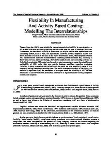
Figure 1 provides a graphical view of the term spreads considered in this study and of the South African (S.A.) business cycle. The shaded areas represent the S.A. recessions according to SARB (2012). Observation of the literature shows that the yield curve inverts prior to the occurrence of an economic recession (Estrella, 2005). The implication is that prior to a recession, the slope of the yield curve becomes negative (otherwise positive – indicating economic growth). Observe from Figure 1 that in the case of S.A., the slope of the yield curve was negative prior to all the recessions. China and U.S. show the same trend. Germany shows a similar trend, however, the large decrease around 2000 was not followed by a recession.

Figure 1: Term Structures Of Interest Rates And S.A. Business Recessions Source: Graphed with the S.A, China, U.S and Germany term spreads and S.A recessions

Table 2 represents the results obtained from testing the term structure data used. The technique used was the Augmented Dickey-Fuller (ADF). The results indicate that the term spread data are l(0) stationary on the level.

624




Volume 12, Number 6

Table 2: Unit Root Testing Results Augmented Dickey-Fuller Unit Root Testing Level Testing t-stats p-value

Term Spreads South Africa c+t -2.998 0.139 c -3.017** 0.037 none -2.783 0.006 United States c+t -4.960* 0.001 c -4.689 0.000 none -2.604 0.001 China c+t -2.874 0.19 c -3.030** 0.048 none -3.105 0.004 Germany c+t -2.348 0.403 c -2.37 0.154 none -2.078** 0.037 Source: Eviews results. Note: (*) indicates that unit root is rejected at 1% significance levels. (**) indicates that unit root is rejected at 5% significance level. (c+t) indicates intercept and trend restriction. (c) indicates intercept restriction. (none) indicates no restrictions

6.2.

Model Results

This section discusses the results of the dynamic probit model estimation for each of the term structures of each country. For each of the term spread in the in-sample forecasting, the model is run with eight different lags (i.e., 1 to 8) and the optimal lag of forecasting is determined from the lag with the highest and lowest Schwartz-Bayesian Information Criteria (SIC), conditional that the RMSE is also the lowest at that particular forecasting lag. Otherwise, the lag with the lowest RMSE is selected as the optimal lag of forecasting for that particular term spread. After the in-sample recession forecasting evaluation of the term spreads, the coefficients of the dynamic probit model estimated in the in-sample estimation are used in the out-of-sample forecasting with the out-of-sample term spread data to predict the South African recessions in the out-of-sample period (i.e., 2001 to 2012) 6.2.1.

The Case For S.A.

6.2.1.1. S.A In-sample Results The in-sample estimation results are presented in Table 3. Table 3: S.A. In-sample Model Estimation Results k=1

k=2

k=3

k=4

k=5

k=6

k=7

k=8

z-statistic p-value

-0.23 -2.78 0.01

-0.27 -3.74 0.00

-0.28 -4.01 0.00

-0.26 -3.81 0.00

-0.22 -3.33 0.00

-0.18 -2.75 0.01

-0.15 -2.33 0.02

-0.11 -1.78 0.08

z-statistic p-value

2.26 5.36 0.00

1.14 3.07 0.00

0.30 0.81 0.42

-0.35 -0.90 0.37

-0.84 -2.12 0.03

-1.11 -2.70 0.01

-1.26 -3.02 0.00

-1.09 -2.83 0.00

0.55 0.94 0.39 0.19

0.39 1.13 0.40 0.27

0.25 1.29 0.43 0.32

0.16 1.39 0.47 0.39

0.13 1.41 0.47 0.47

0.14 1.41 0.48 0.50

0.11 1.44 0.48 0.57

Pseudo 0.74 SIC 0.69 RMSE 0.38 VP 0.10 Source: Eviews Results



625


Volume 12, Number 6

The results indicate that the optimal lag for the best-fit estimation model is at 1 quarter (i.e., when k=1). This is because at this lag, is higher compared to other lags. This is also accompanied by the lowest RMSE, the lowest SIC, and the lowest VP compared to other lags (i.e., from k=2 to k=8). The of 0. 738717 suggest that the S.A. term spread explains about 73% of the variation in the dependent variable. Furthermore the coefficients of both the term spread ( ) and the lagged dependent variable ( ) are statistically significant at 1%, 5% and 10%. Based on the optimal lag selection for the best-fit model criterion set above the following equation represents the estimated in-sample dynamic probit model for S.A. at the optimal lag of k=1:

where F represents the cumulative normal distribution, is the dependent variable that assumes a value of 1 in the event of a recession and 0 otherwise in period t, and is the probability of S.A. being in a recession in period t, given the term spread and lagged dependent variable information, respectively, at time t-1. To illustrate the use of the best-fit model, Table 4 below shows the probabilities of recession given the S.A term spread and recession indicator 1 quarter earlier in the period 1987Q3 to 1999Q2. Table 4 indicates that the probability of S.A. being in a recession was negligible at 1.022% when the term spread averaged 6.555 and the dependent variable was 0. The probability of recession was predicted to be about 13.034%, when the term spread averaged 1.259 and the dependent variable was 0. However, the recession probability was almost certain at 95.611% when the term spread averaged -1.295 and the recession indicator 1. This confirms the observation from the literature that prior to the occurrence of an economic recession, the slope of the yield curve becomes negative (Estrella, 2005). In other words, the probabilities of recession increase.

Quarters Actual Probabilities. %

Predicted Probabilities. (

87/3

%

Table 4: Probabilities Of Recession From The Best-fit Model 87/4 88/1 88/2 88/3 88/4 89/1 89/2 89/3

89/4

90/1

90/2

0

0

0

0

0

0

100

100

100

100

100

6.555

6.556

6.603

5.010

3.530

1.259

-0.120

-1.352

-2.402

-1.660

-1.295

100 1.232

1.022 1.021 0.993 2.442 5.086 13.03 92.54 Source: Calculated Probabilities (=NORMSDIST (

95.72

97.48

96.32

95.61

95.47

))

Figure 2 provides a graphical representation of the in-sample probabilities of the best-fit model for S.A.

Figure 2: Probabilities Of Recession From S.A. Best-fit Model Source: Eviews In-sample Probabilities

Figure 2 provides the probabilities (i.e., on the y-axis) of recessions given the S.A. term spread and recession indicator 1 quarter earlier, as predicted by the in-sample best-fit model (equation 6). The x-axis shows the time frame under review and the shaded sections represent the S.A. recession periods (Moolman 2003), in that time frame (i.e., 1980 to 2000). General observations from Figure 2 are that the best-fit model has predicted all the past 626




Volume 12, Number 6

S.A. recessions that have taken place from 1984 to 2000. The recession in 1982 was only predicted in the middle of the recession while the model produced incorrect probability of recession in 1983. 6.2.1.2. S.A. Out-of-sample Results

Figure 3: S.A. Out-of-sample Expected Versus Actual Probabilities Source: Expected Values Calculated In Excel Using The Best-fit Model

Figure 3 graphically illustrates the probabilities of recessions in S.A. as predicted by the model in the outof-sample forecasting. These expected probability values are plotted against the actual probability values to obtain the comparison between the model predictions and the actual probabilities. General observations from the above plot are that the prediction of the recent S.A. recession of 2008 shows that the probabilities of recession increased immediately after S.A. descended into a recession, correctly indicating the occurrence of a recession. The figure shows that a few quarters before the 2007 recession, the expected probability was already on the rise at above 20%. As S.A. was descending into a recession, the forecast probability increased to above 60% to correctly indicate the occurrence of the recession. During the recession, the expected probability remained above 80%. The plot also illustrates an important feature. The in-sample forecasting of S.A. recessions by Khomo and Aziakpono (2007) produced an incorrect probability of about 84% in 2003, which never took place. However, Figure 3 indicates that the recession probabilities stayed at low levels of just below 40%. This is a more accurate prediction than the insample forecasting, as S.A. did not descend into a recession in 2003. 6.2.2.

In-sample Results Of Foreign Term Spreads

The in-sample results of each of the term spreads are summarized in Table 5. Observe the results for the Chinese term spreads in the table. The optimal lag of the best-fit model given the Chinese term spread and recession indicator 1 quarter earlier is at k =1. This lag is characterized by the highest , the lowest SIC and the lowest RMSE compared to measures at other lags (i.e., from k=2 to k=8). These RMSE and values are similar to those produced by the S.A. best-fit model. At the optimal lag both the coefficients of the term spread and the lagged recession indicator are statistically significant at both 5% and 10% at significant levels. This suggests that the Chinese term spread is best at predicting S.A. recessions, given the Chinese spread and the S.A. recession indicator 1 quarter earlier. As such, the best-fit model for China is presented below:

View the result for the U.S. term spread in Table 5. The optimal lag of the best-fit model is represented by k=5. This is because at this lag, despite the not being the lowest, and the SIC not being the lowest, the lag is selected based on the lowest RMSE compared to other lags. This high RMSE might be due to the fact that the lagged recession variable from an emerging country such as S.A. is modelled with the term spread from a developed country such as the U.S. As such, this suggests that the U.S. term spread predictions of S.A. recessions might not be accurate. As such the best-fit model is as follows:



627


Volume 12, Number 6

Finally, examine Table 5 for the German term spread results. The best-fit model optimal lag is at 8 quarters (i.e., k = 8). Also in this case, the is not the highest and the SIC is not the lowest. But the RMSE is the lowest compared to other lags. The high RMSE suggests that the German term spread might also not be accurate in predicting S.A. recessions. This might be due to a similar reason as in the case for the U.S that the lagged recession variable from an emerging country as S.A is modelled with the term spread from a developed country as Germany. However, the t-statistics is significant at this lag. The best-fit model is represented as follows:

The best-fit models (equation 7, 8, and 9) generate the probabilities of S.A. recessions, given the respective term spreads and the S.A. recession indicator k quarters earlier. Table 5: In-sample Estimations Of Foreign Term Spreads k=1 k=2 k=3 k=4 k=5 k=6

k=7

k=8

CHINA RESULTS

z-statistic p-value

z-statistic p-value Pseudo R-squared Schwartz-Bayesian RMSE Variance Proportion U.S. RESULTS

z-statistic p-value

z-statistic p-value Pseudo R-squared Schwartz-Bayesian RMSE Variance Proportion GERMANY RESULTS

z-statistic p-value

-0.748 -1.863 0.045

-1.105 -1.914 0.056

-1.285 -2.284 0.022

-1.185 -2.279 0.023

-0.908 -1.885 0.059

-0.511 -1.020 0.308

0.400 ---

1.244 ---

2.634 3.167 0.002 0.749 0.919 0.303 0.303

1.695 2.266 0.024 0.596 1.136 0.344 0.253

0.836 1.212 0.225 0.492 1.267 0.366 0.250

0.041 0.061 0.951 0.350 1.426 0.410 0.248

-0.722 -1.031 0.302 0.230 1.544 0.445 0.279

-1.239 -1.601 0.109 0.170 1.582 0.495 0.346

-7.619 --0.401 1.293 0.519 0.148

-7.461 --0.587 1.129 0.334 0.166

0.018 0.124 0.901

-0.119 -1.015 0.310

-0.153 -1.402 0.161

-0.234 -2.137 0.033

-0.271 -2.440 0.015

-0.256 -2.276 0.023

-0.298 -2.407 0.016

-0.204 -1.758 0.079

2.598 6.796 0.000 0.662 0.794 0.513 0.591

1.781 5.436 0.000 0.386 1.136 0.474 0.683

1.141 3.776 0.000 0.189 1.353 0.482 0.684

0.588 2.013 0.044 0.097 1.450 0.479 0.620

0.025 0.087 0.930 0.078 1.469 0.477 0.588

-0.352 -1.199 0.231 0.094 1.453 0.478 0.589

-0.611 -2.034 0.042 0.144 1.400 0.487 0.491

-0.638 -2.133 0.033 0.113 1.436 0.494 0.574

0.026 0.136 0.892

0.027 0.167 0.867

0.087 0.595 0.552

0.153 1.074 0.283

0.238 1.678 0.093

0.342 2.265 0.024

0.410 2.570 0.010

0.444 2.693 0.007

0.964 2.542 0.011 0.100 1.463 0.498 0.640

0.575 1.538 0.124 0.052 1.511 0.493 0.559

0.297 0.772 0.440 0.087 1.474 0.480 0.465

0.015 0.040 0.969 0.154 1.410 0.462 0.422

-0.171 -0.434 0.665 0.207 1.359 0.448 0.406

2.784 1.930 1.400 z-statistic 5.588 4.639 3.581 p-value 0.000 0.000 0.000 Pseudo R-squared 0.701 0.435 0.232 Schwartz-Bayesian 0.759 1.097 1.325 RMSE 0.566 0.492 0.494 Variance Proportion 0.624 0.708 0.700 Source: Eviews results Note: (--) indicates that values could not be computed by Eviews.

628




Volume 12, Number 6

Table 6 below illustrates the use of the Chinese, U.S. and Germany best-fit models in generating the predictions for S.A. recessions in-sample. The term spreads used are in the period from 1995:Q2 to 1998:Q1. Part of the period indicates the time when S.A. was not in a recession (i.e., indicated by 0) and the other part indicates the time when S.A. was in recession (i.e., indicated by 1).

Quarters Actual Prob. (%) CHINA

Table 6: Probabilities Of Recession From The Foreign Best-Fit Models In-sample 95/02 95/03 95/04 96/01 96/02 96/03 96/04 97/01 97/02 97/03

97/04

98/01

0

0

0

0

0

0

100

100

100

100

100

100

0.550

-0.260 15.43 0

-0.530 18.89 0

0.210 10.39 0

0.580

7.550

-0.270 15.59 0

7.330

0.730 86.76 0

-0.020 93.33 0

-0.290 94.94 0

-1.330 98.50 0

-1.110 98.02 0

-1.140 98.10 0

0.630 64.12 0

0.750 62.90 0

0.490 65.53 0

1.180 58.43 0

1.550 54.49 0

1.670 53.20 0

1.250 58.68 0

1.590 55.07 0

1.320 57.94 0

1.000 61.29 0

0.450 66.85 0

0.523 66.13 0

2.390 2.410 1.940 3.050 3.260 3.000 2.660 2.770 2.640 2.410 1.810 75.62 75.89 68.94 83.82 86.00 83.27 73.97 75.53 73.68 70.25 60.45 Prob.( )% 0 0 0 0 0 0 0 0 0 0 0 Source: Calculated Probabilities Using The Best-fit Model Equations (5.2, 5.3 And 5.4) (=NORMSDIST ( ))

1.470 54.54 0

Prob.( )% U.S

Prob.( )% GERMAN Y

Table 6 indicates that in 1995Q2 given the S.A. recession indicator and the Chinese, U.S. and German term spreads at 1, 5 and 8 quarters earlier, respectively, the probabilities were about 7.55%, 64.12% and 75.62%, respectively, that S.A. would be in a recession. Similarly, in 1997Q3 the probabilities were about 98.50%, 61.29% and 70.25%, respectively. As the literature suggests that recessions are signalled by a negatively sloped yield curve, observe from the table above that the slope of the Chinese term spread was positive in the periods of no recessions, from 1995Q2 to 1996Q4. This is indicated by the term spread values increasing in that period until 1996Q4. However, during the recession periods, the slope of the Chinese term spread was positive, indicated by term spread values decreasing until 1997Q3, and started increasing from that period, as S.A. was exiting the recession. Similarly, the U.S. term spread started decreasing from 1997Q1 as S.A. was entering the recession, and began to increase in 1998Q1, indicating a recovery. The probabilities of recession in this period remained above 55%. However, the high probabilities in no recession periods incorrectly predicted the occurrence of a recession. In the case of Germany, despite the negatively sloped yield curve in the recession periods accompanied by high probability levels, the probability levels were as high as about 70% in periods where S.A. was not in a recession. The implication is that the German term spread did not follow accurately the expected behaviour as observed in the literature when forecasting S.A. recessions. Figure 4 provides a graphical representation of the in-sample probabilities generated by the best-fit models of each of the foreign terms spreads:



629


Volume 12, Number 6

Figure 4: Probabilities Of Recessions From The Foreign Best-fit Models In-sample Source: Eviews Prediction In-sample Forecasts

6.2.3.

Out-of-sample Results Of Foreign Term Spreads

Table 7 illustrates the use of the Chinese, U.S. and Germany best-fit models in generating the predictions for S.A. recessions out-of-sample. The term spreads used are in the period from 2006:Q3 to 2009:Q2. Part of the period indicates the time when S.A. was not in a recession (i.e., indicated by 0) and the other part indicates the time when S.A. was in recession (i.e., indicated by 1).

Quarters Actual Prob. (%) CHINA

Table 7: Probabilities Of Recession From The Foreign Best-Fit Models Out-of-sample 06/03 06/04 07/01 07/02 07/03 07/04 08/01 08/02 08/03 08/04

09/01

09/02

0

0

0

0

0

0

100

100

100

100

100

100

0.490

0.340

0.300

0.250

0.510

0.580

0.400

7.190

8.010

9.240

9.560

9.970

7.860

7.330

0.530 90.03 0

0.350 88.85 0

0.170 90.53 0

1.180 91.98 0

1.430 81.25 0

-0.130 61.54 0

-0.210 62.14 0

-0.280 66.83 0

0.390 66.88 0

0.810 67.16 0

0.860 71.48 0

2.150 72.22 0

2.280 72.89 0

2.900 66.44 0

2.050 62.19 0

2.470 61.77 0

3.340 49.03 0

0.600 0.400 0.300 0.600 0.300 0.500 -0.200 0.600 -0.300 0.600 68.80 63.10 62.80 53.90 54.10 53.10 57.40 59.70 46.50 42.80 Prob.( )% 0 0 0 0 0 0 0 0 0 0 Source: Calculated Probabilities using the best-fit model equations (5.2, 5.3 and 5.4) (=NORMSDIST (

2.000 41.40 0

2.800 46.20 0 ))

Prob.( )% U.S

Prob.( )% GERMANY

Table 7 shows that in the period from 2006Q3 to 2007Q4 in which S.A. was not in a recession (i.e., indicated by actual probability values of 0%), the Chinese best-fit model produced probabilities lower than 10%, providing correct probabilities of recessions. However, the U.S. and German best-fit models generated probabilities higher than 50%, incorrectly forecasting the occurrence of the recent recession of 2008. Moreover, in the time horizon in which S.A. was in a recession from 2008Q1 to 2009Q2 (i.e., indicated by actual values of 100%), the probabilities generated by the Chinese best-fit model increased from below 10% in 2008Q1 to above 80% in all the recessionary quarters, correctly forecasting the S.A. recession. The probabilities generated by the U.S. model remained above 60% and decreased from 2009Q2, while the German probabilities decreased to below 50% during 630




Volume 12, Number 6

the recession. The U.S. produced some correct signals of the recessions but also provided incorrect signals in the periods in which S.A. was not in a recession. However, in the case of Germany the probabilities are countercyclical. In periods of no recession, the probabilities are high and in recession periods, the probabilities are low. Figure 5 provides a pictorial view of the out-of-sample prediction performance.

Figure 5: Probabilities Of Recessions From The Foreign Best-fit Models Out-of-sample

Source: The Calculated out-of-sample Probabilities 6.3.

Comparative Analysis Between The S.A. Term Spread And Foreign Term Spreads Predictions Table 8 presents the in-sample and out of sample RMSE values of each best-fit model for each country. Table 8: The In-sample And Out-of-sample Forecasting RMSE Values S.A CHINA U.S.

GERMANY IN-SAMPLE RMSE 0.3798 0.3035 0.4772 0.4476 OUT-OF-SAMPLE RMSE 0.450 0.580 0.163 0.101 Source: in sample RMSE obtained from Eviews. For out-of-sample, expected probabilities for each quarter calculated using the best-fit models (=NORMSDIST ( )). The RMSE is then the average of the square root of the error squares at each quarter (i.e., error = actual probability – expected probability).

As discussed, both S.A. and China derive their best-fit estimation models at a lag of 1. This means that both China and S.A. can best forecast the S.A. recessions, given their spread levels and the S.A. recession indicator 1 quarter earlier. Equal optimal lags of forecasting between these countries may be due to the fact that S.A. and China are both emerging markets, and hence closely linked to each other. This link is indicated by the fact that China is regarded by the SARS as the number one country of destination for S.A. value-add export. Moreover, Laribee (2008) maintains that the bilateral economic ties between S.A. and China are due to the large-scale trade and investment deals which flow between the two countries. In fact, in May 2008 China became South Africa’s largest investing foreign country (Laribee, 2008). This suggests that a drastic decline in investment trading between S.A. and China would affect foreign revenue streams into S.A. and hence impact its economic activity with almost immediate effect. However, in the case of the U.S. and Germany the best-fit model is derived from the optimal lag of 5 and 8, respectively. Observe in Table 8 that both the U.S. and Germany generate higher values of RMSE of about 0.4772 and 0.4476, respectively, compared to S.A. and China. The high values of RMSE compared to those of S.A. and China might be due to the fact that the lagged recession indicator of a developing country such as S.A. was used with the term spread of developed countries such as the U.S. and Germany. The high RMSE values suggested that 2013 The Clute Institute Copyright by author(s) Creative Commons License CC-BY 631


Volume 12, Number 6

the U.S. and German term spreads might not accurately forecasts future S.A. recessions. In the case of the U.S. this was evident from Section 6.2.1, that the U.S. provided some false signals of the S.A. recessions in some quarters. However, the German best-fit model provided mixed signals in which in most cases the model generated high probabilities in non-recession periods and low probabilities in recession periods. As such, the German model did not provide accurate forecasts of future S.A. recessions; in fact the generated probabilities were countercyclical. Table 8 shows that the out-of-sample RMSE values of S.A. (0.163) and China (0.101) are low. This was evident with the predicted out-of-sample expected probabilities predicting the direction of the actual probabilities (Figure 5), particularly closely matched by the Chinese probability graph. This suggested that the S.A. and Chinese spreads are able to accurately forecast S.A. recessions given their respective spreads and the S.A. recession indicator 1 quarter earlier. However, the RMSE values are once again high for the U.S. (0.4550) and Germany (0.580) in the out-of-sample forecasting, particularly for Germany. This suggested that even the real-world forecasting of the U.S. and Germany might not accurately predict the S.A. recessions 7.

SUMMARY OF FINDINGS AND RECOMMENDATIONS

7.1.

Summary

As observed in the literature, market interest rates usually move in the same direction as business cycles. Market interest rates usually rise when the economy is expanding towards its highest point, and tend to fall as the economy declines towards its lowest point or recession (Rose, 2003). The expectations theory asserts that when the yield curve is upward-sloping, short-term interest rates are expected to increase in the future; and when the yield curve is downward-sloping, short-term interest rates are expected to decline in the future. An upward-sloping yield curve is induced when long-term interest rates are higher than the short-term interest rates. Similarly, a downwardsloping yield curve is produced when the short-term interest rates are higher than the long-term interest rates. The inversion of the yield curve prior to the 1988 and 1989 recessions in the U.S. has been documented in the literature and, as such, the yield curve has been qualified by economists, researchers and policymakers as one of the prominent tools to use in forecasting future economic activities (Estrella, 2005). Many of the studies are based on the U.S., but a considerable number on Brazil, Canada, Australia, New Zealand, and Germany also exist. The emphases in these studies is that the yield curve dominates other macroeconomic variables in forecasting future economic activities and recessions, particularly in the longer time horizons of more than two quarters into the future. 7.2.

Concluding Remarks

The S.A. term structure of interest rates has not lost its ability to forecast S.A. recessions due to the several reasons. First, in the in-sample (i.e., from 1989 to 2000) forecasting, the S.A. best-fit model was able to accurately forecast all the recessions (i.e., 1980, 1984, 1986, and 1996) given the level of the term spread and the recession indicator 1 quarter earlier. Second, the out-of-sample forecasting findings revealed that the S.A. best-fit model again accurately predicted the occurrence of the S.A. 2008 recession. Finally, the out-of-sample predictions revealed that the incorrect predictions of 2003 by Khomo and Aziakpono (2007) were indeed incorrect since the probabilities of recessions remained below 40%, correctly indicating a non-recession period for S.A. The Chinese best-fit model performed better than the S.A. best-fit model in predicting the 2007 recession about a quarter before its occurrence. The RMSE of 0.101 by the Chinese best-fit model was lower than the RMSE of 0.163 by the S.A. best-fit model. The implication is that economists and policymakers alike might also benefit a great deal from the predictive power of the Chinese term spreads in terms of forecasting S.A. recessions. With regard to the U.S., the best-fit model provided recession signals about five quarters before the 2007 recession, but also gave incorrect signals of recession around 2002. In the case of Germany, the best-fit model produced countercyclical recession signals. This indicated that in the real world, the German term spread does not predict S.A. recessions. The study illustrated and confirmed that S.A. and China are closely linked emerging market countries as indicted by Laribee (2008). This was illustrated by the fact that both S.A. and Chinese term spreads could better 632




Volume 12, Number 6

forecast the S.A. recessions; given their respective term spread levels and recession indicators one quarter earlier. Moreover, the best-fit models accurately forecast the S.A. recessions, both in-sample and out-of-sample, with China performing better than S.A. in the out-of-sample forecasting. 7.3.

Limitations Of The Study

Due to the poor availability of the Chinese data prior to 1995, this study was unable to investigate the ability of the Chinese term spread in forecasting S.A. As such, this study was not able to entirely compare the forecasting ability of the Chinese best-fit model with that of the S.A. best-fit model in-sample. 7.4.

Research Recommendation

Considering the above-mentioned limitation of the study in Section 7.3, it could be worthwhile and useful if one could investigate the predictive power of the Chinese term spread prior to 1995, firstly because it would provide a complete comparative analysis with the forecasting ability of the S.A. term spreads and secondly, if the Chinese term spreads prove to have accurately signalled the S.A. recession prior to 1995, the policymakers could use the Chinese term spreads to validate the recession forecasts of the S.A. term spreads. Furthermore, the research illustrated that between 2003 and 2004 the yield curve decreased below zero and had a negative slope. However, the out-of-sample analysis showed that the probability of recession was below 40% in that period. If one could analyse the economic factors that lead to this occurrence, it might provide a better understanding of the economic dynamics that lead to this observation. AUTHOR INFORMATION Ilsé Botha holds a D.Com (Economics) degree from the University of Johannesburg – previously Rand Afrikaans University. Before entering academia, she worked as an economist at a Bank. She is currently a senior lecturer at the Department finance and investment management at the University of Johannesburg where she teaches and supervise at the postgraduate level. She is involved in various research projects and her current research explores various time series techniques and business cycle economics. E-mail: [email protected] (Corresponding author) Tjhaka Alphons Mohapi, Department of Economics and Econometrics; University of Johannesburg, South Africa; Alphons Mohapi is an analyst at a prominent Bank. He completed his Masters studies last year at the University of Johannesburg. REFERENCES 1.

2. 3. 4. 5. 6. 7. 8. 9.

Alessandrini, F. (2003). Do Financial Variables Provide Information About the Swiss Business Cycle? University of Lausanne, Department of Economics. Retrieved from http://www.hec.unil.ch/deep/textes/03.02.pdf Bernard, H., & Gerlach, G. (1996). Does the Term Structure Predict Recessions? The international evidence. Bank for Internationl Settlements, Working paper no. 37, September. Bonser-Neal, C., & Morley, T. (1997). Does the yield spread predict real economic activity? A multicountry analysis. Federal Reserve Bank of Kansas City Economic Review, 3rd Quarter, pp.37-53. Brunetti, M., & Torricelli, C. (2009). Economic activity and recession probabilities: information content and predictive power of the term spread in Italy. Applied Economics, 41, p.2309–2322. Burns, A.F., & Mitchell, W.C. (1946). Measuring business cycles. Journal of the American Statistical Association, 41(236), p.599-602. Dotsey, M. (1998). The predictive content of the interest rate term spread for future economic growth. Federal Reserve Bank of Richmond Economic Review, 3rd Quarter, pp.31-51. Dueker, M.J. (1997). Strengthening the Case for the Yield Curve as a Predictor of US Recessions. Federal Reserve Bank of St. Louis. Economic Review, 79, pp.41-51. Dueker, M.J. (2005). Dynamic forecasts of qualitative variables: a qual VAR model of U.S. recessions. Journal of Business and Economic Statistics, 23, p.96–104. Estrella, A., & Hardouvelis, G.A. (1991). The Term Structure as a Predictor of Real Economic Activity. The Journal of Finance, 46(2), pp.555-76.



633

International Business & Economics Research Journal – June 2013 10. 11. 12. 13. 14. 15. 16. 17. 18. 19. 20. 21.

22. 23. 24. 25. 26. 27. 28. 29. 30. 31. 32. 33. 34. 35. 36. 37. 634

Volume 12, Number 6

Estrella, A., & Mishkin, F.S. (1995). The Structure of Interest Rates and its Role in Monetary Policy for 15. European Central Bank. Federal Reserve Bank of New York, Working paper no.9526, September. Estrella, A., & Mishkin, F.S. (1996). The Yield Curve as a Predictor of U.S. Recessions. Current Issues in Economics and Finance, 2(7), pp.1-6. Estrella, A., & Mishkin, F.S. (1998). Predicting U.S. Recessions: Financial Variables as Leading Indicators. The Review of Economics and Statistics, 80(1), pp.45-61. Fung, A., & Chapple, B. (1994). The Yield Curve As An Indicator Of Monetary Conditions. Reserve Bank Bulletin, 57(1), pp.35 -45. Gowland, D. (1991). Money, Inflation and Unemployment. The Role of Money in the Economy. 2nd ed. New York: Harvester Wheatsheaf. Gujarati, D.N. (2003). Basic Econometrics. 4th ed. Boston: McGraw-Hill Irwin. Hao, L., & Ng, E.C.Y. (2011). Predicting Canadian recessions using dynamic probit modelling approaches. Canadian Journal of Economics, 44(4), p.297–1330. Haubrich, J., & Dombrosky, A. (1996). Predicting real growth using the yield curve. Federal Reserve Bank of Cleveland Economic Review, 32, 1st Quarter, pp.26-34. Howells, P.G.A., & Bain, K. (1994). Financial markets and institutions. 2nd ed. United States of America, New York: Addison Wesley Longman Limited. Howells, P., & Bain, K. (1998). The Economics of Money, Banking and Finance, A European Text. Essex, England: Pearson Educational Limited. Hubbard, R.G. (2008). Money, the financial system, and the economy. 6th ed. Boston: MA: Pearson. Karunaratne, N.D. (1999). The Yield Curve as a Predictor of Growth and Recessions in Australia. Discussion Papers in Economics and the Economic Issues series, The University of Queensland, no. 255, May. Kauppi, H., & Saikkonen, P. (2008). Predicting U.S. recessions with dynamic binary response models. Review of Economics and Statistics, 90(4), p.777–791. Khomo, M.M., & Aziakpono, M.M. (2007). Forecasting Recessions in South Africa: A Comparison of The Yield Curve and other Economic Indicators. South African Journal of Economics, 75(2), pp.194-212. Laribee, R. (2008). Trade Supply within the Chinese Diaspora in South Africa. Africa Spectrum, 43(3), pp.353-70. Michaelsen, J.B. (1965). The Term Structure of Interest Rates and Holding-Period Yields on Government Securities. The Journal of Finance, 20(3), pp.444-63. Mishkin, F.S. (2004). The Economics of Money, Banking and Financial Markets. International Edition ed. New York: Pearson Addison-Wesley. Moneta, F. (2003). Does the yield spread predict recessions in the euro area? European Central Bank Working Paper No. 294, December. Moneta, F. (2005). Does the Yield Spread Predict Recessions in the Euro Area? International Finance, 8(2), p.263–301. Moolman, E. (2002). The Term Structure as a Predictor of Recessions. Journal for Studies in Economics and Econometrics, 26(6), pp.43-51. Moolman, E. (2003). Predicting Turning Points in the South African Economy. South African Journal of Economic and Sciences, 6(2), pp.289-303. Moore, G.H. (1967). What is a Recession? The American Statistician, 21(4), pp.16-19. National Bereau of Economic Research. (2001). The Business-Cycle Peak of March 2001. NBER. [Online] Available: http://www.nber.org/reporter/fall01/ [Accessed 10 April 2012] Nel, H. (1996). The term structure of interest rates and economic activity in South Africa. The South 44. African Journal of Economics, 63(3), pp.161-74. Nyberg, H. (2010). Dynamic Probit Models and Financial Variables in Recession Forecasting. Journal of Forecasting, 29, pp.215-30. South African Reserve Bank. (2012). SARB. Quartely Bulletin. Retrieved from http://www.resbank.co.za/Publications/QuarterlyBulletins/Pages/QuarterlyBulletins-Home.aspx South African Revenue Services. (2012). SARS. Quartely Report. Retrived from http://www.sars.gov.za/home.asp?pid=4150 Stojanovic, D. & Vaughan, M. (1997). Yielding clues about Recessions: The Yield Curve as a Forecasting Tool. Federal Reserve Bank of St. Louis. Copyright by author(s) Creative Commons License CC-BY


The Explanatory Power Of The Yield Curve In ... - Clute Institute

The Explanatory Power Of The Yield Curve In ... - Clute Institute

Suggest Documents

Enron - The Clute Institute

Analysis - The Clute Institute

The Goal - Clute Institute

Title - The Clute Institute

Introduction - The Clute Institute

Fitting the yield curve - YieldCurve.com

The Yield Curve - Secret Agent

Learning Through the Yield Curve

In The Service Sector - The Clute Institute

In The Service Sector - The Clute Institute

Brownyn A - The Clute Institute

Bankruptcy Prediction - The Clute Institute

CRISIS MANAGEMENT - The Clute Institute

Foreign Currency - The Clute Institute

Sarbanes Oxley - The Clute Institute

AIS Salaries - The Clute Institute

Jennifer Styron - The Clute Institute

Cytotec: the future - Clute Institute

cultural diversity - The Clute Institute

cultural diversity - The Clute Institute

table 1 - The Clute Institute

newhorizonsinadultedu cation - The Clute Institute

Demystifying Clouds - The Clute Institute

CPS Energy - The Clute Institute