MATEC Web of Conferences 63, 04045 (2016)
DOI: 10.1051/ matecconf/20166304045
MMME 2016
The generation algorithm of arbitrary polygon animation based on dynamic correction a
Ya Wei Hou , Yong Gang Li, Jin Biao Zhou, Jian Wei He and Yu Xin Zhang China Satellite Maritime Tracking and Controlling Department, Jiangyin 214431, Jiangsu, China
Abstract. This paper, based on the key-frame polygon sequence, proposes a method that makes use of dynamic correction to develop continuous animation. Firstly we use quadratic Bezier curve to interpolate the corresponding sides vector of polygon sequence consecutive frame and realize the continuity of animation sequences. And then, according to Bezier curve characteristic, we conduct dynamic regulation to interpolation parameters and implement the changing smoothness. Meanwhile, we take use of Lagrange Multiplier Method to correct the polygon and close it. Finally, we provide the concrete algorithm flow and present numerical experiment results. The experiment results show that the algorithm acquires excellent effect. Key words: Animation, Polygon,Vectors,Correction
Fundamental assumption and Define The deformation process of polygon, without
Introduction As the base of computer animation techniques, two-dimensional animation is a research highlights of current computer science. Two-dimensional animation can be implemented through boundary polygon deformation, so the main mathematical model of two-dimensional animation is polygon deformation techniques. That is to say, in some method to design medium growing change process, the initial object continuously changes to target object on the vision. It is also called 2D-Shape blending. Polygon deformation techniques is widely applied in many fields, such as computer graphics, virtual reality, industry simulation, visualization in scientific computing, bio-medical engineering and so on. And it has already been the important part of computer animation techniques. As an emerging research field, it is with important academic value and research value.
a
considering the effect of adjacent cycle, need to meet following conditions. (a) the track of feature points of polynomial(generally the peaks of polynomial) in change period is continuous, smooth and fairing; (b) the length of polynomial sides is monotonous in change period. In the process to implement continuous animation, in order to make the polygon continuously transit in different change periods, we need to weaken condition (b) according to requirements, so as to achieve the continuity of deformation track during different periods. This
paper,
for the sake of convenience in researching,
we
instructions
following
symbols.
for
the
A = [ A0 , A1 ,LL , A n ,LL]
T = [T0 , T 1 ,LL , Tn ,LL]
,
give
, with
Corresponding author:
[email protected]
© The Authors, published by EDP Sciences. This is an open access article distributed under the terms of the Creative Commons Attribution License 4.0 (http://creativecommons.org/licenses/by/4.0/).
MATEC Web of Conferences 63, 04045 (2016)
DOI: 10.1051/ matecconf/20166304045
MMME 2016
Ak = {ak ,1 , ak ,2 ,LL , ak ,n } . Ak ,i means the peak i of
the
state
polygon
k,
and
record
λk , s ∈ (−1, ∞),θ k , s ∈ (0, ∞)
as
t is the mapping of [Tk −1 , Tk ] in unit interval
∆Tk := Tk − Tk −1 . Bk (t ) is continuous deformation sequence of
Ak −1 → Ak . That is to say, the polygon
continuous change sequence interval
[0,1] .As Fig 1, the physical significance of second interpolation vector defined by (1) is that vector’s terminal point track is quadratic Bezier curve of
(k = 1, 2,3.L) in
pk , s − ak −1, s
[Tk −1 , Tk ] , in the form of edge vector is
vectors.
Bk (t ) = {bk ,1 (t ), bk ,2 (t ),L , bk , n (t )} .
ak , s − pk , s
as
feature
pk , s − ak −1, s and ak , s − pk , s form feature
polygon of interpolation curve. Vector
Second interpolation edge-vector
and
method
of
bk , s (t ) keeps good continuity and smooth
in deformation period. But in initial deformation period, it is necessary to consider the monotony of vector
Define second interpolation vectors of
ak −1, s and
length. For first-order continuously differentiable curve
bk , s (t ) ,it has following theorem:
ak , s
Theorem 1: the sufficient and necessary condition bk , s (t ) = (1 − t ) ak −1, s + 2t (1 − t ) pk , s + t ak , s t∈[0,1] (1) 2
2
for
Among them:
| bk , s (t ) | as monotonous on [0, 1] is that
(bk' , s (t ), bk , s (t )) on [0,1] keeps same symbole.
pk , s = (1 + λk , s )(ak −1, s + θ k , s ak , s ) / 2
Figure 1 quadratic Bezier interpolation of
Figure 2 quadratic Bezier interpolation
edge-vector
based on dynamic correction smooth and fairing cannot be realized. Therefor,in order to hold the polygon deformation smooth during
Dynamic correction of interpolation parameter
animation restructuring procedure, every edge-vector need
The quadratic Bezier curve defined by the method
meet
deformation
mentioned above, keeps good characteristics. It only meet the continuation in adjacent periods,while the
2
first-order
continuity
during
whole
process.That
MATEC Web of Conferences 63, 04045 (2016)
DOI: 10.1051/ matecconf/20166304045
MMME 2016 is,
dbk −1, s (t ) dT
|T =Tk −1 =
dbk , s (t ) dT
According to the characteristic of polygon,if polygon
|T =Tk −1 ,according to
Bk (t ) meets the closed condition, it is necessary
Bezier curve characteristic, Bezier curve and its characteristic
polynomial’s
first
and
last
n
∑b
side
s =1
respectively tangent to the initial and ending points,and the tangent vector is n times of edge-vector.That is:
2(ak −1, s − pk −1 ) ∆Tk −1
=
2( pk − ak −1, s ) ∆Tk
θk ,s =
∆Tk −1 [2 − (1 + λk −1, s )θ k −1, s ] + 1 ∆Tk
(t ) = 0 .
So, we could make correction on
(2)
adjustment
It can get from above formula:
λk , s =
k ,s
edge-vector ,
of
on
it,
and
Bk (t ) ,
polygon
then
as
that
is
bk*, s = bk , s + ηk , s And then we could get:
∆Tk (1 + λk −1,s ) 2∆Tk −1 + ∆Tk [2 − (1 + λk −1, s )θ k −1, s ]
n
∑ [b s =1
The interpolation curve
ηk ,s
amount
bk , s and add
got
k ,s
(t ) + ηk , s ] = 0 .
Define function
from above formula could meet deformation smooth as
n
ϕ (η k ,1 ,η k ,2 ,L ,ηk , n ) = ∑ (bk , s (t ) + η k , s ) = 0 ( 4 ) s =1
T = Tk . But because of randomness of time sequence,
Objective
pk , s cannot be guaranteed to fall over the first
function n
ηk2, s
s =1
| bk , s (t ) |2
f (ηk ,1 ,ηk ,2 ,L ,η k ,n ) = ∑
quadrant of affine coordinate system built by
ak , s , ak +1, s .So it is necessary to conduct limit to above
.It needs to
ηk , s , and make f reach its minuteness
confirm all
formula:
is
under the constrain condition (4).Using Lagrange
∆Tk −1 λk , s = max( ∆T [2 − (1 + λk −1, s )θ k −1, s ] + 1, −1) ( 3 ) k ∆Tk (1 + λk −1, s ) θ = max( , 0) k , s 2∆Tk −1 + ∆Tk [2 − (1 + λk −1, s )θ k −1, s ]
multiplicator method, take λ as multiplicator, and command
Φ(λ ,ηk ,1 ,ηk ,2 ,L ,η k ,n ) = f + λϕ .
From equation set As shown by Figure 3, the first method is the
this algorithm. By comparison, during polygon
∂Φ ∂λ = 0 ∂Φ =0 ∂ηk , s
animation restructuring procedure,the method in this
It can be got:
results by general second interpolation according to Guozhao Wang, and the second method is the results by correction on interpolation parameters according to
paper could make the transition much smooth and
n
fairing in different periods.
ηk ,s =
Polygon closure correction
bk2, s (t )∑ bk ,i (t ) i =1
n
∑b i =1
2 k ,i
(5)
(t )
The polygon formed by above method cannot completely close.That is to say,it is not real sense of
Therefore, the edge-vector of polygon on time t is
polygon. Therefore, we need to amendment the results.
3
MATEC Web of Conferences 63, 04045 (2016)
DOI: 10.1051/ matecconf/20166304045
MMME 2016 the method proposed in this paper implement the
n
* k ,s
b (t ) = bk , s (t ) +
bk2, s (t )∑ bk ,i (t ) i =1
n
∑b i =1
2 k ,i
smooth and fairing of animation, and the effect is 。 ( 6 )
excellent.
(t ) References
Thus we could calculate polygon
Bk (t ) .
[1] Zhao-guo Wang, Bao-gang Bai, Ruo-feng Tong, A vector blending approach for computer animation .J. Chinese Journal of Computers. 12 (1996). 881-886.
Numerical experiment result
[2] LEE T Y, HUANG Pohua. Fast and intuitive
There are many experiments using the method
metamorphosis of 3D polyhedral models using SMCC
mentioned above. As Figure 4, it is the deformation
mesh merging scheme .J. IEEE Transition
animation from Chinese character “凹”to a circular.
Visualization and Computer Graphics, 2003, 9 (1) :
st
The 1 ,3
rd
and 8
th
frame is polygon key-frames of
85-98.
T=0,T=0.4,T=1.4. The other frames is polygon
[3] The method of computer aided geometric design.
reconstructed by the method stated in this paper. We
Xi’an , Northwestern poly-technical university
can see from the figure,for the implement of polygon
press,1986.
sequence animation with time attributes, polygon
[4]Ya-Qing Xu, Bao-gang Bai, UNRBS as a new
gradual changing method based on dynamic correction
application of animation vector mixed method. J.
can achieve the effect of smooth, fairing and natural
Journal of Xinjiang Petroleum Institute 12(2000):69-74
transition.
[5] Chang-xu Dou ,Yu-mei Wang , Quadratic Interpolation Deformation Algorithm of Polygon Central Point Vector. J. Computer Engineering . 2010.36(16):189-191
Figure 3 Deforming animation from Chinese character ‘凹’ to circular
Conclusion This paper proposes one method of polygon animation implement based on dynamic correction. Firstly, vectorize the metamorphosis polygon,and then carry out second interpolation to corresponding edge-vector, meanwhile in the interpolation process, keep
first-order
continuity
of
edge-vector
and
peak-point track, and to the greatest extent maintain the monotony of side.And then, by means of dynamic correction for interpolation parameters, implement continuous
transition
and
fairing
in
different
deformation periods.Finally,correct the deformation edge-vector which uses least square method to close the polygon. Numerical experiment results indicate that
4