Nov 27, 2017 - review the use of the κ-framework, fiducial and simplified template cross .... II.2 Observables for probing Higgs boson recoil . ...... For this reason, the BFM provides a good bookkeeping framework that can ...... nc (q1,q2), (I.98).
IPPP/17/90
The HiggsTools Handbook: Concepts and observables for deciphering the Nature of the Higgs Sector Abstract
arXiv:1711.09875v1 [hep-ph] 27 Nov 2017
This Report summarizes some of the activities of the HiggsTools Initial Training Network working group in the period 2015-2017. The main goal of this working group was to produce a document discussing various aspects of state-of-the-art Higgs physics at the Large Hadron Collider (LHC) in a pedagogic manner. The first part of the Report is devoted to a description of phenomenological searches for New Physics at the LHC. All of the available studies of the couplings of the new resonance discovered in 2012 by the ATLAS and CMS experiments [1, 2] conclude that it is compatible with the Higgs boson of the Standard Model (SM) within present precision. So far the LHC experiments have given no direct evidence for any physical phenomena that cannot be described by the SM. As the experimental measurements become more and more precise, there is a pressing need for a consistent framework in which deviations from the SM predictions can be computed precisely. Such a framework should be applicable to measurements in all sectors of particle physics, not only LHC Higgs measurements but also electroweak precision data, etc. We critically review the use of the κ-framework, fiducial and simplified template cross sections, effective field theories, pseudoobservables and phenomenological Lagrangians. Some of the concepts presented here are well known and were used already at the time of the Large Electron-Positron Collider (LEP) experiment. However, after years of theoretical and experimental development, these techniques have been refined, and we describe new tools that have been introduced in order to improve the comparison between theory and experimental data. ∗
In the second part of the Report, we propose φη as a new and complementary observable for studying Higgs boson production at large transverse momentum in the case where the Higgs ∗ boson decays to two photons. The φη variable depends on measurements of the angular directions and rapidities of the two Higgs decay products rather than the energies, and exploits the information provided by the calorimeter in the detector. We show that, even without tracking ∗ information, the experimental resolution for φη is better than that of the transverse momentum of the photon pair, particularly at low transverse momentum. We make a detailed study of the ∗ phenomenology of the φη variable, contrasting the behaviour with the Higgs transverse momentum distribution using a variety of theoretical tools including event generators and fixed order perturbative computations. We consider the theoretical uncertainties associated with both pT H ∗ ∗ and φη distributions. Unlike the transverse momentum distribution, the φη distribution is well predicted using the Higgs Effective Field Theory in which the top quark is integrated out – even ∗ at large values of φη – thereby making this a better observable for extracting the parameters of ∗ the Higgs interaction. In contrast, the potential of the φη distribution as a probe of new physics is rather limited, since although the overall rate is affected by the presence of additional heavy ∗ fields, the shape of the the φη distribution is relatively insensitive to heavy particle thresholds.
i
Authors 1
2
3,4
2
2,5
M. Boggia , J. M. Cruz-Martinez , H. Frellesvig , N. Glover , R. Gomez-Ambrosio , 1 2,6 7,8 1,9 5,10 2 1 G. Gonella , Y. Haddad , A. Ilnicka , S. Jones , Z. Kassabov , F. Krauss , T. Megy , 11,12 2 5 13,14,15 16 D. Melini , D. Napoletano , G. Passarino , S. Patel , M. Rodriguez-Vazquez , 17 T. Wolf 1 2
3
4
5
6 7
8 9
10
11
12 13 14
15
16
17
Physikalisches Institut, Albert-Ludwigs-Universität Freiburg, 79104 Freiburg, Germany Institute for Particle Physics Phenomenology, Department of Physics, University of Durham, Durham DH1 3LE, UK Institute of Nuclear and Particle Physics, NCSR “Demokritos”, Agia Paraskevi, 15310, Greece Institute for Theoretical Particle Physics (TTP), Karlsruhe Institute of Technology, Engesserstraße 7, D-76128 Karlsruhe, Germany Dipartimento di Fisica Teorica, Università degli Studi di Torino and INFN, Sezione di Torino, Via Pietro Giuria 1, 10125 Turin, Italy High Energy Physics Group, Blackett Lab., Imperial College, SW7 2AZ, London, UK Institute for Theoretical Physics, University of Zürich, Winterthurerstrasse 190, 8057 Zürich, Switzerland Institute for Particle Physics, Physics Department, ETH Zürich, 8093 Zürich, Switzerland Max-Planck-Institut für Physik, Werner-Heisenberg-Institut, Föhringer Ring 6, 80805 München, Germany Dipartimento di Fisica, Università degli Studi di Milano and INFN, Sezione di Milano, Via Celoria 16, 20133 Milan, Italy Departamento de Física Teórica y del Cosmos, Avenida de la Fuente Nueva S/N C.P. 18071 Granada, Spain IFIC, Universitat de València and CSIC, Catedrático Jose Beltrán 2, 46980 Paterna, Spain DESY, Notkestrasse 85, 22607 Hamburg, Germany Institute for Theoretical Physics (ITP), Karlsruhe Institute of Technology, WolfgangGaede-Straße 1, D-76131 Karlsruhe, Germany Institute for Nuclear Physics (IKP), Karlsruhe Institute of Technology, Hermann-vonHelmholtz-Platz 1, D-76344 Karlsruhe, Germany Laboratoire de Physique Théorique, UMR 8627, CNRS, Université de Paris-Sud, Université Paris-Saclay, 91405 Orsay, France Nikhef, Science Park 105, 1098 XG Amsterdam, The Netherlands
Acknowledgements We thank Ramona Gröber for useful comments, and Xuan Chen, Aude Gehrmann-De Ridder, Thomas Gehrmann, Alex Huss and Tom Morgan for their collaboration in developing the NNLOJET code. We thank Marzieh Bahmani, Giulio Falcioni, Nicolas Gutierrez, Brian Le, Elisa Mariani, Joosep Pata and Cosimo Sanitate for their contributions to the HiggsTools Initial Training Network. We gratefully acknowledge the Research Executive Agency (REA) of the European Union for funding through the Grant Agreement PITN-GA-2012-316704 (“HiggsTools”). M.B. and G.G. acknowledge the German Research Foundation (DFG) and Research Training Group GRK 2044 for the funding and the support.
ii
Contents I
Towards a theory of Standard Model deviations
1
I.1
Introduction . . . . . . . . . . . . . . . . . . . . . . . . . . . . . . . . . . . . . . . .
1
I.2
The κ-framework . . . . . . . . . . . . . . . . . . . . . . . . . . . . . . . . . . . . .
3
I.3
Fiducial and simplified template cross sections . . . . . . . . . . . . . . . . . . . . .
15
I.4
Effective field theories
. . . . . . . . . . . . . . . . . . . . . . . . . . . . . . . . . .
25
I.5
Pseudoobservables for the LHC . . . . . . . . . . . . . . . . . . . . . . . . . . . . .
46
I.6
Tools and phenomenological Lagrangian . . . . . . . . . . . . . . . . . . . . . . . .
60
I.7
Summary . . . . . . . . . . . . . . . . . . . . . . . . . . . . . . . . . . . . . . . . . .
70
II
∗
φη : A new variable for studying H → γγ decays
71
II.1
Overview . . . . . . . . . . . . . . . . . . . . . . . . . . . . . . . . . . . . . . . . . .
71
II.2
Observables for probing Higgs boson recoil . . . . . . . . . . . . . . . . . . . . . . .
76
II.3
Photons . . . . . . . . . . . . . . . . . . . . . . . . . . . . . . . . . . . . . . . . . .
81
II.4
Parton Showers . . . . . . . . . . . . . . . . . . . . . . . . . . . . . . . . . . . . . .
85
II.5
Theoretical Predictions . . . . . . . . . . . . . . . . . . . . . . . . . . . . . . . . . .
88
II.6
Beyond the Standard Model . . . . . . . . . . . . . . . . . . . . . . . . . . . . . . . 115
II.7
Summary . . . . . . . . . . . . . . . . . . . . . . . . . . . . . . . . . . . . . . . . . . 124
A
Calculation of the One-Loop Master Integrals . . . . . . . . . . . . . . . . . . . . . 125
B
Two-loop Feynman Integrals
. . . . . . . . . . . . . . . . . . . . . . . . . . . . . . 132
iii
Chapter I Towards a theory of Standard Model deviations I.1
Introduction
Before the discovery of the Higgs boson in 2012, the hypothesis under test at the LHC was the Standard Model (SM) with the Higgs boson mass, mH , being the unknown parameter. Therefore, bounds on mH were derived through a comparison of theoretical predictions with high-precision data. Now, after the discovery, the SM is fully specified and the unknowns are constrainable deviations from the SM. Of course, the definition of SM deviations requires a characterization of the underlying dynamics. So far, all of the available studies of the couplings of the new resonance conclude that it is compatible with the Higgs boson of the SM with our current precision, and, as of yet, there is no direct evidence for new physics phenomena beyond the SM at the LHC. This chapter is devoted to a description of phenomenological searches for New Physics (NP) at the LHC. Some of the concepts presented here are well known and were used already at the time of the Large Electron-Positron Collider (LEP). Now, after years of developments both on the experimental and the theoretical sides, these techniques have been refined, and new tools have been introduced in order to improve the comparison of theory to experiment. In this work, different approaches are revisited, with special emphasis on the relations and connections between them, showing their limits, and how they complement each other. In the following we will introduce their main definitions, necessary for a complete comprehension of the chapter. The technical details will be largely covered in the following sections. The κ-framework The κ-framework was proposed shortly after the discovery of the Higgs boson in order to try a systematic and model-independent search for SM deviations. It is used at Leading Order (LO) and accommodates for factorisable Quantum Chromodynamic (QCD) corrections but not for Electroweak (EW) ones. The κ-framework will be covered in Section I.2, where its use during the Run 1 of the LHC is discussed and its limitations highlighted. Fiducial and Simplified Template Cross Sections Fiducial cross sections are useful observables for particle physics, but they have always been a source of disagreement between theorists and experimentalists. The reason is that the phase space defined by the theory is not the same as the one of the detector and additionally, different detectors operate at their maximum efficiency in different regions of the phase space. The Simplified Template Cross Sections (STXSs) are one of the possible answers to this problem. They provide a gain in experimental sensitivity by introducing a small theoretical model dependence. STXSs are defined in greater detail in Section I.3. Effective Field Theories (EFTs) EFTs come into play when the solutions to a quantum field theory are provided as expansions in a small coupling constant and ratio of scales. Among these theories the Standard Model EFT (SMEFT) is an example. In such theories an infinite number of higher dimensional operators must be included, which means that the theory is (strictly) non-renormalisable. Nevertheless, 1
if v is the Higgs vacuum expectation value and E is the typical scale at which the process is measured, the EFT amplitudes are expanded in powers of v/Λ and of E/Λ, where Λ is the scale of new physics. This expansion is computable to all orders and the introduction, order-by-order, of an increasing number of counter-terms can eliminate the UV divergences, which makes the theory renormalisable order-by-order in the E/Λ perturbative expansion. An overview of EFTs is presented in Section I.4 introducing definitions, descriptions and methodologies. Pseudoobservables (POs) Pseudoobservables were introduced to allow a better interplay between theory and experiment. They answer the urgent need of extending the parameters of the κ-framework to something with a more rigorous theoretical interpretation. Another main advantage of POs is that they deliver results which do not have to be totally unfolded by experiments to a model-dependent parameter space. POs could also be the solution to the issue posed by the κ-framework of not being able to describe theoretically any eventual SM deviations (being only able to parametrise but not to explain such measurements), and at the same time, POs make it possible to get closer to quantities that are well defined QFT objects. POs had been already used for LEP analysis, and they have gained new relevance now given their close connection with EFTs. They are addressed in Section I.5 as a natural continuation of Section I.4. Phenomenological Lagrangians Several models have been built that aim at producing observable NP effects based on phenomenological Lagrangians constructed by adding a limited number of additional interactions to the SM Lagrangian. Theoretical tools and Monte Carlo (MC) generators with such implementations are already available. Section I.6 offers an insight into this topic, together with a discussion of the challenges faced when dealing with Next-to-Leading Order (NLO) corrections. Finally, there are a couple of finer points in terminology that are worth keeping in mind: 1) technically speaking leading-order defines the order in perturbation theory where the process starts. Sometimes, however, “LO” is used in the literature to denote tree level (as opposed to loop contributions). 2) The resonant (often called “signal”) and the non-resonant (often called “background”) are parts of a physical process (which may contain more than one resonant part). Typically whenever we write i → X → f we mean the X -resonant part of a process with initial state i and final state f . However, we should keep in mind that separating and defining “signals” and “backgrounds” is not trivial. For example, V h production at LO in QCD with V → jj and Vector Boson Fusion (VBF) are not clearly separated. At Next-to-Next-to-Leading Order (NNLO) QCD everything becomes much more complicated and even the definition of V h, V → jj and VBF is ambiguous.
2
The κ-framework
I.2 I.2.1
Concept and description
Theory and experiment aim at the same goal but, surprisingly, they often find it hard to communicate with each other. The search for a common language to be used by experimentalists to express their results and by theorists to interpret them has become more and more urgent after the observation of a massive neutral boson [1,2], that is identified as being compatible with the quantum fluctuations of a field whose Vacuum Expectation Value (VEV) breaks the EW symmetry. This is the well-known Brout-Englert-Higgs mechanism of Refs. [3–8] and the LHC resonance has been interpreted so far in terms of the SM Higgs boson. The Higgs boson couplings to the other known particles play a central role in the investigation of the properties of this state, since they are predicted very accurately by the SM and its extensions. They also influence the Higgs boson production and decay rates: this is why an interim framework called the κ-framework was proposed in Ref. [9] to parameterise small deviations from the predicted SM Higgs boson couplings and widths, for a recent review see Ref. [10]. The basic assumptions are: – The signals observed in the different search channels originate from a single narrow resonance with a mass near 125 GeV. – The zero-width approximation is used, meaning that the total width of the resonance is narrow enough to be negligible with respect to the mass. In this case, the signal cross section can be decomposed (for all i → H → f channels) as f
σi · BR =
σi · Γf , ΓH
(I.1)
where σi is the production cross section for i → H with i = (ggF, VBF, W H, ZH, tt¯H) f and BR is the decay Branching Ratio (BR) for H → f with f = (ZZ, W W, γγ, τ τ, bb, µµ). Γf and ΓH are the partial and total decay widths of the Higgs boson respectively. The couplings cannot be directly measured by the experiments and events collected in the detector undergo an unfolding procedure, in order for us to be able to extract the information from some measurable observable(s). Typically, the measured observable is σ × BR, which is defined within a certain acceptance and with some specific experimental cuts, and this leads to some model dependence. Obviously, it is not possible to fit the experimental data within the context of the SM while treating Higgs couplings as free parameters. Once the value of the Higgs boson mass is specified, the couplings are specified as well. For this reason, it is only possible to test the overall compatibility of the SM with the data. This kind of study can be used to extract or constrain deviations in the measured couplings with respect to the the SM ones. Some of the available approaches introduce specific modifications in the structure of the couplings: besides including all the available higher order corrections in the model, they add additional terms to the Lagrangian, the so-called “anomalous couplings”. This gives rise to modifications of the tensor structure of the amplitude leading not only to a modification of the coupling strengths, but also of the kinematic distributions. This approach has turned out to be a difficult one when it comes to reinterpreting the results. An additional assumption is then made to simplify the framework: – The tensor structure of the couplings is assumed to be the same as in the SM predictions, only modifications of coupling strengths are taken into account. This implies that the observed state is assumed to be a CP-even scalar. 3
The framework is built in such a way that the predicted SM Higgs cross section and partial decay widths are dressed with scaling factors κj , as shown in Table I.1. The cross section σi 2 2 and the partial decay width Γf scale with κi , κf when compared to SM predictions. 2
f
f
σi · BR = (σi · BR )SM ·
2
κi · κf 2
κH
.
(I.2)
In the SM, all the κi are unity by definition and therefore, the best available (i.e. highest possible perturbative order) predictions are recovered. However, when κi 6= 1 higher-order accuracy is in general lost due to the factorisation of Eq.(I.2) does not necessarily hold beyond LO. This will be illustrated later on with an example. The κ are sometimes confused with the actual couplings in the Lagrangian. They are the same at tree level, but not the same once radiative corrections are taken into account. As an example we consider the process gg → tt¯H(bb). At tree level one can say that the squared matrix elements are proportional to the coupling of the interactions: 2
2
|M| ∝ (gtH gbH ) ,
(I.3) SM
and then, assuming that the total width of the Higgs boson stays unchanged, ΓH ≡ ΓH , one would have κi = gtH and κf = gbH . Another quantity that can be expressed in this framework and is a common experimental observable, is the signal strength µ. Consider a specific process i → H → f . For the production (i → H) the signal strength µ is defined as µi =
σi , σiSM
(I.4)
whereas, for the decay (H → f ) we have µf =
BR
f
f
.
(I.5)
BRSM
By definition, in the SM µi = 1 and µf = 1. The only thing that can be measured experimentally is the product of µi and µf , since it is not possible to separate them without further assumptions. In terms of the κ-framework we obtain the following expression: 2 2
µ ≡ µi µf ≡
κi κf 2
κH
.
(I.6)
To summarize, the original κ-framework is a simplified picture which shows its limitations when more precise data necessitate the inclusion of higher order QCD and EW corrections. In many cases, the QCD corrections do not completely factorise and their impact in the context of the SMEFT can be sizeable, as was shown in Ref. [11]. Keeping this in mind, let us first discuss the LO strategy, which was applied during the analysis of the LHC Run 1 data. Different production processes and decay modes probe different coupling modifiers. Together with the individual modifiers related to the coupling of the Higgs boson with different particles, two effective modifiers need to be introduced to describe loop induced processes: the modifier κg to describe the ggF production process and κγ for the H → γγ decay.
4
Production σ(ggF) σ(VBF) σ(W H) σ(qq/qg → ZH) σ(gg → ZH) σ(tt¯H) σ(gb → tHW ) σ(qq/qb → tHq) σ(b¯bH)
Effective Loops Interference scaling factors
Resolved scaling factors
X − − − X − − − −
t− b − − − t−Z − t−W t−W −
κg − − − − − − − −
2
1.06 · κt + 0.01 · κb + 0.07 · κt κb 2 2 0.74 · κW + 0.26 · κZ 2 κW 2 κZ 2 2 2.27 · κZ + 0.37 · κt − 1.64 · κZ κt 2 κt 2 2 1.84 · κt + 1.57 · κW − 2.41 · κt κW 2 2 3.40 · κt + 3.56 · κW − 5.96 · κt κW 2 κb
2
2
− − X − − −
− − t−W − − −
− − 2 κγ − − −
κZ 2 κW 2 + 0.07 · κt − 0.66 · κW κt 2 κτ 2 κb 2 κµ
−
2 κH
Partial decay width ΓZZ ΓW W Γγγ Γτ τ Γbb Γµµ
2
2
1.59 · κW
Total width (BRBSM =0) 2
ΓH
X
2
2
0.57 · κb + 0.22 · κW + 0.09 · κg + 2 2 2 0.06 · κτ + 0.03 · κZ + 0.03κc + 2 2 0.0023 · κγ + 0.0016 · κ(Zγ) + 2 0.0001 · κs + 0.00022 · κµ
Table I.1: Higgs boson production cross sections σi , partial decay widths Γf , and total decay width (in the absence of BSM decays) parametrised as a function of the κ coupling modifiers, including higher-order QCD and EW corrections to the inclusive cross sections and decay partial widths. The coefficients in the expression for ΓH do not sum exactly to unity because some negligible contributions are not shown. Table from Ref. [12].
This is possible since it is expected that other Beyond the SM (BSM) particles which might be present in the loop do not change the kinematics of the process. The study of these processes can therefore be approached by either using effective coupling modifiers, which provide sensitivity to the presence of BSM particles in the loops, or using resolved coupling modifiers corresponding to the SM particles. I.2.2
The κ-framework in the experiments
The measurement of the properties of the Higgs boson is one of the main goals of the two LHC general purpose experiments: ATLAS, described in Ref. [13], and CMS, described in Ref [14]. For the interpretation of results in the light of a combination it is mandatory to have a global overview of the current situation and to understand how the κ-framework has been used by the experiments so far. In the following we review the combination of measurements performed by the ATLAS and CMS experiments, which was presented in Ref. [12], with a focus on the constraints on the couplings. The analysis used the data collected by the detectors from pp collisions at the LHC in 2011
5
√ −1 and 2012, corresponding to an integrated luminosity of approximately 5 fb at s = 7 TeV and √ −1 20 fb at s = 8 TeV. They considered multiple production processes: gluon fusion, vector boson fusion, and associated production with a W or a Z boson or a pair of top quarks, and 1 the H → ZZ, W W , γγ, τ τ , bb and µµ decay modes. Two formalisms were used to interpret the results: the signal strength µ, related to the yields, and the κ-framework for the couplings. Usually, Higgs cross section measurements are given in two ways: – Fiducial cross-section: this has basically no input from the signal Monte Carlo (MC), so it can be compared to any theory calculation, provided that it can reproduce the cross-section within these specific cuts – Signal strength (µ). In this case, – The event yield after cuts is computed. – This is extrapolated to the full phase space using signal Monte Carlo (typically POWHEG [15] + JHUGen [16–19] + Pythia8 [20]+ Geant4 [21]) in the full detector simulation to compute acceptance and efficiency. – The result is compared with the best theory predictions, e.g. Next-to-Next-to-Nextto-Leading Order (N3LO) QCD for production in the gluon fusion channel, and Prophecy4f, from Refs. [22–24], for decays with four fermions in the final state. To directly measure the individual coupling modifiers, an assumption for the Higgs boson width is necessary. It is predicted to be approximately 4 MeV in the SM, which is assumed to be small enough for the Narrow Width Approximation (NWA) to be valid and for the Higgs boson production and decay mechanisms to be factorised. The relations among the coupling modifiers, the production cross-sections and the partial decay widths of Table I.1 are used as a parametrisation to extract the coupling modifiers from the measurements. Changes in the values of the couplings will lead to a change of the Higgs 2 boson width. To characterise this variation a new modifier κH is introduced, defined as κH = P j 2 2 j BR SM κj . If we only allow for SM decays of the Higgs boson, the relation κH = ΓH /ΓH;SM holds, otherwise ΓH can be expressed as: 2
ΓH
κH · ΓH;SM = , 1 − BRBSM
(I.7)
where BRBSM indicates the total branching fraction into BSM decays. Since ΓH is not experimentally constrained in a model-independent manner with sufficient precision, only ratios of coupling strengths can be measured in the most generic parametrisation considered in the κframework. The individual ATLAS and CMS analysis of the Higgs boson production and decay rates are combined using the profile likelihood method. Intermezzo: profile likelihood method The statistical data treatment used in the combination is the same as that used by the single analysis and described in Ref. [25]. Let us consider a kinematic variable x and the corresponding histogram of values n = (n1 , . . . nn ). The expectation value in a bin i can be written as Z
E[ni ] = µsi + bi ,
where si = stot
bin i
Z
fs (x, θs )dx ,
bi = btot
bin i
fb (x, θb )dx ,
(I.8)
and µ determines the strength of the signal process, with µ = 0 being the background-only hypothesis and µ = 1 the nominal signal hypothesis. 1
Note that the definition of the H → ZZ(W W ) decay requires some additional information.
6
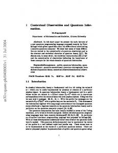
Fig. I.1: Best fit values of ratios of Higgs boson coupling modifiers, as obtained from the generic parametrisation. The single results from each experiment are also shown. The thick error bars indicate the 1 σ interval and the thin lines the 2 σ one. The hatched areas indicate the nonallowed regions for the parameters that are assumed to be positive without loss of generality. For those parameters with no sensitivity to the sign, only the absolute values are shown. Figure from Ref. [12].
The functions fs (x, θs ) and fb (x, θb ) are the probability density functions of the variable x for signal and background characterised by the set of parameters θ~s and θ~b . The quantities stot and btot are the total mean numbers of events for signal and background: stot is not considered to be an adjustable parameter but rather fixed to the value predicted by the nominal signal model. In addition to the histogram of interest n, supporting measurements are usually made to help constrain the nuisance parameters. Therefore for a control sample where mainly background is expected, we may find a histogram m = (m1 , ..., mM ) for a particular kinematic variable, where the expectation value of mi is E[mi ] = ui (θ) . (I.9) Here the ui are calculable quantities that depend on θ = (θs , θb , btot ). This is often done to obtain information on the parameter btot . In each bin, the number of events follows the Poisson distribution and the likelihood function is the product of those probabilities for every bin, L(µ, θ) =
m n N M Y uk k −uk (µsi + bi ) j −(µsi +bi ) Y j=1
e
nj !
k=1
mk !
e
.
(I.10)
The likelihood function is then used to build a so-caled “test statistic” Λ(µ) =
ˆ L(µ, ˆ θ) , ˆ L(ˆ µ, θ)
7
(I.11)
ˆ where ˆ θ indicates the value of θ that maximizes L for a specific value of µ (conditional maximumlikelihood estimator for θ), while µ ˆ and θˆ are the unconditional maximum likelihood estimates of the parameter values. Likelihood fits are then performed to obtain the values for the parameters of interest. The actual data is used for the observed values and Asimov datasets, see for instance Ref. [25], are used for the expected values. Asimov datasets are pseudo-data distributions equal to the signal plus background predictions for a given value of the parameters. By definition, when the Asimov dataset is used to estimate the parameters, the “true” values are obtained. Often, not all of the parameters need to be estimated and in these cases a profile likelihood analysis is performed, which means that the parameters one is not interested in are written as a function of the parameters of interest. The combination is based on simultaneous fits to the data from both experiments taking into account the correlations between systematic uncertainties within each experiment and between the two experiments. Almost all input analysis are based on the concept of event categorisation. This consists of classifying the events in different categories, based on their kinematic properties. This categorisation increases the sensitivity of the analysis and also allows separation of the different production processes on the basis of exclusive selections that identify the decay products of the particles produced in association with the Higgs boson: W or Z boson decays, VBF jets, etc. A total of approximately 600 exclusive categories addressing the five production processes explicitly considered are defined for the five main decay channels. The signal yield in a category k, nsignal (k), can be expressed as a sum over all possible Higgs boson production processes i, with cross section σi and decay modes f , with branching f fraction BR : nsignal (k) = L(k) ·
XXn i
= L(k) ·
f
f
σi · Ai;SM (k) · �i (k) · BR
o
f
XX i
f
n
f
f
f
o
(I.12)
µi µf σi;SM · Ai;SM (k) · �i (k) · BRSM ,
f f
where L(k) represents the integrated luminosity, Ai;SM (k) the detector acceptance assuming f
SM Higgs boson production and decay, and �i (k) the overall selection efficiency for the signal category k. Finally µi and µf are the production and decay signal strengths, respectively. It can be seen that the measurements are only sensitive to the products of the cross sections f and branching fractions, σi · BR . The overall statistical methodology is the same as used by the single experiments. The parameters α are estimated via the profile likelihood ratio test statistics Λ(α), which depend on one or more parameters as well as on the nuisance parameters, θ, which reflect various experimental and theoretical uncertainties. The likelihood functions are constructed using products of signal and background Probability Density Functions (PDFs) of the discriminating variables. The probability density functions are obtained from simulations in the case of the signal and from both data and simulation for the background case. Three parametrisations of experimental results have been performed in the combination: two are based on cross-sections and branching fractions, one is based on ratios of couplings modifiers. The σ · BR for gg → H → ZZ channel is parametrised as a function of κgZ = κg · κZ /κH (where κg is the effective coupling modifier). The measurement of VBF and ZH production probes λ = κZ /κg , the measurements of tt¯H production processes are sensitive to λtg = κt /κg . The three decay modes H → W W , H → τ τ and H → bb probe the three ratios λW Z = κW /κZ , λτ Z = κτ /κZ and λbZ = κb /κZ , relative to the H → ZZ branching fraction. 8
S F¯1 F2
+
hf¯i fj
χf¯i fj
m
i − 2s 2IW,f Mf,i δij
3
1 f,i CL − 2s M δij W
φ u ¯i dj
m
W
m
3 mf,i i 2s 2IW,f MW δij
1 f,i CR − 2s M δij W
mu,i √1 V 2s MW ij m − √12s Md,j Vij W
− φ d¯j ui m
†
− √12s Md,j Vji W
mu,i † √1 V 2s MW ji
Table I.2: Scalar-fermion couplings in the SM, from Ref. [26].
Other parametrisations were performed in the combination analysis with more specific and more restrictive assumptions. I.2.3
Limitations of the κ-framework
One problem that arises at higher orders is the violation of unitarity. Unitarity is connected to the renormalisability of a theory, and the introduction of coupling modifiers for the Higgs spoils unitarity and renormalisability. Example H → b¯ b decay width To show why the κ-framework cannot be considered a fully consistent theoretical framework, we give an example of the problems arising when we try to compute an observable at NLO precision in this framework. We consider a “simplified κ-framework” phenomenological Lagrangian, similar to the Lagrangian that is discussed in Section I.6.2. We define this simplified theory as follows: we start from the SM (following here the conventions of Ref. [26]), and we modify all the fermionic couplings to scalar particles, multiplying them by a common factor κf f S . In this simplified framework, the generic scalar-fermion vertex is given by F¯1
�
h
= ie κf f S
1 − γ5 1 + γ5 CL + CR , 2 2 �
(I.13)
F2
where the values of the coefficients CL and CR are specified in Table I.2. As for the observable that we want to compute, we consider the Higgs decay width into a pair of bottom quarks, i.e. Γ(H → b¯b). The Born matrix element for the decay process reads as follows: M0 =
e mb κf f S u ¯(p)v(k) , 2sMW
(I.14)
and we can see how the LO SM decay width is modified using this simple phenomenological 2 model: it is rescaled by a factor κf f S coming from the square of Eq. (I.14). This rescaling reflects the effects of the κ-framework on the fermion-fermion-Higgs coupling. To achieve a more accurate theoretical prediction, we must include contributions containing higher powers of the coupling constant α. The NLO matrix element can be cast in the following form, see for example Ref. [27], � �� � α (I.15) δ + δCT , M = M0 1 + 4π loop where δloop contains the contributions due to loops with internal gauge and Higgs bosons, and δCT the counterterm contributions coming from the renormalisation procedure. In this example, the purpose is not to show the complete derivation of the NLO decay width, but we want to highlight the NLO inconsistency of the κ-framework. To this end, we take
9
b
b
b h
h
h
h
φ
b
b
b
b
b
b
Z h
t
W h
b Z
φ b
h Z
b h
b
W
b
W
χ
W
h t
b h
b χ
b
Z t
b
Z
b
b
b
t
b
b
φ
b
b h
b χ
h
b γ
h
b
b
b
t
h
φ t
b
b χ
h
b
b
h
h
b b
φ
b
t χ
b
h
b
b
b
t W
b
b
(a) b h b
(b)
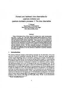
Fig. I.2: (a) Loop contributions to the Higgs decay into a bottom quark pair. (b) Counterterm contribution to the Higgs decay into a bottom quark pair.
advantage of the following simplifications: firstly, we drop QCD contributions, and we focus on the EW corrections. Then, by means of dimensional regularisation, we identify the UV divergent contributions in the NLO matrix element, and we drop the UV finite part. This allows us to overlook the problems related to the infrared (IR) and collinear structure of the loop amplitude (involving the inclusion of the real emission process H → b¯b(γ, g)). Finally, we neglect effects induced by the quark-mixing matrix V in the W -boson couplings of Table I.2, setting Vij = δij . For the renormalisation procedure, we adopt the on-shell scheme, as presented in Ref. [28]. In this scheme, each renormalised mass is related to the corresponding physical mass, defined as the real part of the particle propagator pole. Considering EW corrections, δloop of Eq. (I.15) contains contributions coming from the diagrams reported in Fig. I.2a and δCT , the counterterm contribution reported in Fig. I.2b. The UV-divergent part of δloop turns out to be (in the MS scheme) 1
δloop UV =
36 s
2
2 MW
2 2 2 2 2� 26MW + MZ + 18 κf f S mt , 4−D
(I.16)
where D is the number of space-time dimensions considered to regularise the loop integrals, and the factor 2/(4 − D) shows the divergent contribution. To motivate this result, we can separate the loop contributions into four different classes, ordered as they appear in Fig. I.2a: I. scalar-exchange diagrams, where a scalar particle is exchanged between the two outgoing b quarks, II. diagrams with two scalars running in the loop, 10
III. diagrams with one internal gauge boson line (exchanged by outgoing particles, or emitted by the incoming Higgs), IV. diagrams with two gauge boson lines running in the loop. As can be seen by naive power counting, type-II and type-IV diagrams are UV finite and do not 2 contribute to δloop . Conversely, type-I and III render UV contributions that are respectively 3 2 0 proportional to κf f S and κf f S , leading to κf f S and κf f S terms in Eq. (I.16). The counterterm contribution, written in terms of renormalisation constants, is given by α δZ δZ s 1 2 δCT = − AA + H − δZZA − 2 2 δMW 4π 2 2 2c 2s MW 2
−
c
2s
2 2 δMZ
+
d,L
1
2 2 2 δMW s MZ
(I.17)
d,R
δmb δZ33 + δZ33 + + , mb 2
where the renormalisation constants are fixed by the scheme chosen in the renormalisation d,L(R) procedure. In the on-shell scheme, the field renormalisation constants δZAA , δZH , δZ33 are related respectively to the one-loop self-energies of the photon, the Higgs boson, and the 2 bottom quark. Consequently, in the considered framework, we expect κf f S contributions in the d,L(R)
renormalisation constants δZH and δZ33 , due to the presence of scalar-fermion couplings in the one-loop self-energies of the Higgs boson and the bottom quark. The expression for the constant δZAA , related to the photon self-energy, in which the modified couplings do not appear, will reproduce the SM result. Repeating the same argument, 2 we can argue that among the other constants, only δmb will present a κf f S term. This is reflected in the expressions of the renormalisation constants, and their UV divergent parts:
δZi UV =
2 α dZ , 4 − D 4π i
(I.18)
with, 2
dMZ = dZAA 2
dMW
dmb = d,L
d,R
dZ33
�
2
2
−3MZ
2
�X
2
ml + 3
X
2 ml
X
2
�
2
2
4
4
�
mq − 70MW MZ + 22MW + 47MZ ,
6MW s q l 4MW 23 , = − , dZZA = 3 MZ s �X � X 2 �� 1 2 2 2 mq , = − 2 7MW − 6MZ + 3 ml + 3 6s q l
dZH =
dZ33
1
1
�
2
2MW s
2 2 −κf f S
+3
� 2
2
�
2 mq
�
+
2 2MW
+
2 MZ
�
,
(I.19)
q
l
mb 2
�X
2
2
�
2
2
�
9κf f S mb − mt + 2MW + 7MZ ,
24MW s � � � � 1 2 2 2 2 2 =− 9κ m + m + 26M + M ffS b t W Z , 2 2 36MW s � � 1 2 2 2 2 =− 9m κ − 2M + 2M . b f f S W Z 2 2 18MW s
The compensation of divergent terms between loop diagrams and counterterms, when performing the renormalisation procedure is a delicate mechanism. We will see how the presence of κdependent terms spoils the cancellation of the divergent part. µ
2
Except for the W -exchange diagram, which is UV-finite because of the γ (1 − γ5 ) structure of the W coupling to two fermions.
11
Indeed, the UV component of the counterterm contribution, obtained inserting Eq. (I.19) into Eq. (I.17), is the only source of divergences that might compensate the UV component of δloop given in Eq. (I.16), rendering the one-loop matrix element UV finite and thus valuable for the evaluation of the decay width. The substitution leads to δCT
UV
=−
1 2
2
36 s MW +
2 9 κf f S
� �X X 2� 2 2 2 2 26MW + MZ − 9 ml + 3 mq 4−D q l �
2 2mt
+
X
2 ml
+3
X
2 mq
��
(I.20)
,
q
l
and we see that the one-loop corrected transition matrix element of Eq. (I.15) gets a UV divergent contribution � X 2� α M0 2 2 � X 2 M UV = ml + 3 mq , (I.21) 2 4 − D 1 − κf f S 4π 4s2 MW q l which in general does not vanish for κf f S 6= 1. Another unsatisfactory aspect of using the κ-framework is that it cannot describe deviations in differential distributions. This happens because global factors can predict how many times the Higgs decays in a specific channel, but not how the kinematics of the decay products are affected. Of course new physics could modify these differential distributions, but it would not be captured by the overall factors. The κ-framework is well motivated if one is looking for large deviations from the SM, as was the case in Run 1. The kappas parametrise these deviations and, if something new would be found, they would point which direction one should look into. ATLAS and CMS did not find any large differences in what was predicted by the SM, therefore the next step would be looking for small deviations. I.2.4
Extrapolation on achievable experimental accuracy in future Runs
It starts to become clear that defining a theoretical framework able to describe possible deviations in the Higgs sector is not straightforward. If one wants to be as model independent as possible, an EFT approach may be the answer. EFTs will be extensively discussed in Section I.4, however, here we demonstrate how the testable hierarchies of scales are limited by the experimental accuracy. The maximum testable hierarchy of scales is determined by two “sources”: the assumption 3 of a maximum size of underlying couplings and the experimental precision In the EFT approach and for observables close to the on-shell Higgs region, the higher dimensional operators are 2 2 2 ordered by factors g mH /Λ (where Λ is the scale of the momentum cut-off of the theory), i.e. the only relevant scale for “on-shell” Higgs production is given by mH . This scale should be well separated from the experimentally accessible scale, in our case the EW scale Λ � v . The applicability of an EFT approach is, however, limited when the hierarchy of scales is not guaranteed. Because hadron colliders do not have a well-defined partonic energy, strategies relying on boosted objects and large recoils are the most critical. While it is not clear that a marginal separation of scales invalidates the EFT approach, such observables clearly pose a challenge. For this reasons, interpreting LHC physics in terms of an effective theory involves a delicate balance between energy scales. It is possible to roughly estimate the physics scales which can 3
The problem for the interpretation of results in terms of an EFT during Run 1 was indeed the limited experimental accuracy, see Ref. [29].
12
be probed, and see if the deviation from the SM Higgs production and decay rates lies within the experimental accuracy. For instance in the energy region around the Higgs peak, 2 2 σ × BR g mH = − 1 2 . (σ × BR)SM Λ
(I.22)
The accuracy on a rate measurement can then be translated into a threshold for new physics as 2 2 σ × BR g mH = − 1 > ∆. 2 (σ × BR)SM Λ
(I.23)
This translates into the following relation: gm Λ < √ H. ∆
(I.24)
The precise value of the experimental accuracy ∆ depends on the process under consideration. If we assume a value of ∆ = 10% (which roughly covers the current experimental accuracy), 2 then for a weakly interacting theory with g ∼ 1/2, one can probe scales up to Λ ≈ 280 GeV. This means that for weakly coupled new physics and with current experimental accuracy, it is not possible to test very high energy scales. However, for a more strongly interacting theory with g ∼ 1 (but g < 4π, which is the theoretical limit for preserving unitarity), one can probe higher scales up to Λ ≈ 400 GeV. The increased statistics and Higgs production cross sections at Run 2 will enable us to add a wide range of distributions and off-shell processes to the Higgs observables, which can probe higher energy scales Λ � mH . It is important to note that, if we look at differential observables, and in particular in the tails of the distributions, Eq. (I.24) has to be modified by substituting mH → pT . Depending on the pT regions that are reconstructed by the experiment, we will be able to access also different Λ values. Of course, we have to keep in mind that when we move 2 towards higher Q , the accuracy on the measurement will drastically decrease, and the value of ∆ has to be reconsidered. Intermezzo: Higgs off-shellness In the NWA, ΓH 7 GeV, |η| < 2.47 pT > 6 GeV, |η| < 2.7
pT > 7 GeV, |η| < 2.5 pT > 5 GeV, |η| < 2.4
pT > 20, 15, 10, 10 GeV
pT > 20, 10, 7(5), 7(5) GeV
Lepton definition Electrons Muons Event selection Leptons pT cuts
+
Invariant masses cuts
Lepton separation
−
+
−
50 GeV < m(l , l ) < 106 GeV 0− 0+ 12 GeV < m(l , l ) < 115 GeV + − 0− 0+ 118 GeV < m(l , l , l , l ) < 129 GeV + − m(l , l ) > 5 GeV
40 GeV < m(l , l ) < 120 GeV 0− 0+ 12 GeV < m(l , l ) < 120 GeV + − 0− 0+ 105 GeV < m(l , l , l , l ) < 140 GeV + − m(l , l ) > 4 GeV
∆R(li , lj ) > 0.1(0.2) for same(opposite) sign
∆R(li , lj ) > 0.02 for every i 6= j
Table I.3: Some of the differences in the definition of fiducial volumes for ATLAS, defined in Ref. [35] and CMS, defined in Ref. [36] for the H → 4l analysis.
Of course the definitions of the physical objects have to be shared between the various experiments and fiducial volumes have to be the same in order for all quantities to be comparable. This is not obvious, since each experiment could be in principle most sensitive to an observable in a different region of the phase space than others. As an example, in the ATLAS and CMS analysis of H → 4l, published in Refs. [35,36], the fiducial cuts are similar but not precisely the same - see Table I.3. Global combinations can be done by correcting to a common fiducial volume. This procedure introduces a small theoretical dependence, but the benefits of the combinations are much larger, as discussed in Section I.2.2. In some cases, it is necessary to simply extrapolate the measurement to a larger phase space, because the definition of minimally-theory dependent fiducial phase space is not possible. In that case, the formula for the fiducial cross section becomes: fid
(σi )exp =
Nev,if , αif �if L
(I.33)
where we introduced the factor αif which extrapolates the measurement to the larger fiducial phase space. A study of the extrapolation and unfolding factors can be found in Ref. [36] from the CMS analysis of H → 4l and is reported in Table I.4 with the notation used in this section. Table I.4 shows that the acceptance factors depend strongly on the Higgs production modes, and that the unfolding factors are compatible within their errors, because the different production modes have very different kinematics and final states. Thus, it makes sense to report Higgs fiducial cross sections in large fiducial volumes in terms of Higgs production modes. A last thing to notice is that in Eq. (I.33), the experimental and theoretical uncertainties factorise. In fact, a naive calculation of the relative error on the fiducial cross section gives: ∆σ σ
fid
fid
=
∆αif ∆Nev ∆�if ⊕ 2 ⊕ 2 . Nev �if αif
(I.34)
When a more precise measurement becomes available, there is no need to repeat the analysis from the beginning. Only the extrapolation factors αif need to be re-computed, starting from the unfolded distribution. To summarise, the new framework for Higgs physics should: – Measure cross sections. – Unfold cross sections to fiducial volumes, taking advantage of positive aspects of fiducial measurements while not renouncing to maximise experimental sensitivity. 18
αif
Signal process
�if
Higgs production modes 0.422 ± 0.001 0.476 ± 0.003 0.342 ± 0.002 0.348 ± 0.003 0.250 ± 0.003
ggH V BF WH ZH ttH
0.681 ± 0.002 0.678 ± 0.005 0.672 ± 0.003 0.679 ± 0.005 0.685 ± 0.010
Non-SM models CP
−
q q¯ → H(J =1 ) CP + q q¯ → H(J =1 ) ∗ gg → H → Zγ ∗ ∗ gg → H → γ γ
0.238 ± 0.001 0.283 ± 0.001 0.156 ± 0.001 0.238 ± 0.001
0.642 ± 0.002 0.651 ± 0.002 0.667 ± 0.002 0.671 ± 0.002
Table I.4: Fiducial volume and detector/unfolding efficiencies and their errors, for H → 4l. Table from Ref. [36].
– Yield cross section measurements in terms of production modes, since acceptance factors depend on them. The simplified template cross section (STXS) framework, introduced in Ref. [37] is designed to take these considerations into account. It tries to combine the ease with which signal-strengthlike fits are performed experimentally with the theoretical needs of fitting to well defined and calculable predictions, aiming to find a good compromise between theory-independence of the measurements and their experimental sensitivity. The STXS framework will be explained in detail in the next section. I.3.3
Simplified template cross section framework
STXSs are fiducial cross sections defined in simplified fiducial volumes. The definition of the fiducial volumes allows the use of advanced experimental techniques, thereby gaining in experimental sensitivity, at the cost of a small dependence on the theoretical model. This is necessary, since at the moment all the measurements on Higgs boson cross sections are dominated by statistical uncertainty. Also the combination of different decay channels reduces the statistical uncertainty. This has been shown, for example, in Ref. [38], where the combination reduced the statistical error on the production cross section by a factor of 1.4. ∆σ ∆σ (H → γγ) = 35% , (H → ZZ) = 23% , σ σ ∆σ (H → γγ ⊕ H → ZZ) = 17% . σ
(I.35)
Combining the different Higgs decay channels would further improve the precision of the measurements. This is the main difference between the usual fiducial differential cross sections and the STXS framework. While fiducial measurements maximise the independence on the theoretical modelling, simplified cross sections maximise the experimental sensitivity. Instead of using fully differential distributions, cross sections are divided into sub-cross sections, called bins. How to choose such bins is an interesting topic in its own right and is discussed in Section I.3.4. The definition of the physics objects in the STXS fiducial volume, is aimed at taking advantage of combinations. It is independent of the Higgs decay modes in such a way that 19
Fig. I.4: Parton level (left), usual particle level definition (center) and corresponding particle level definition for STXSs (right), for the tt¯H production mode. Blue blobs represent particles −10 with long lifetime (& 10 s).
combinations do not introduce further theory dependent factors. In STXS, the particle level is defined with undecayed Higgs bosons while jets are reconstructed from the particles which are not associated with the Higgs decay. The formula connecting single channel measurements to the STXS is: f
i
f
i
α
σi (exp) = Af,α1 σi 1 α α2
σi (exp) = Af,α1 α2 σi 1
(I.36)
··· f
α α2 ···αn
i
σi (exp) = Af,α1 α2 ···αn σi 1
,
where i={ggF , V BF , V H, ttH, bbH, tH} and f ={b¯b, γγ, ZZ, W W , τ τ } denote production α α α α α ···α f and decay modes respectively, σi 1 , σi 1 2 , σi 1 2 n are the STXSs and the Ai,α1 α2 ···αn are efficiency/acceptance factors for each STXS. Each line of Eq. (I.36) is called a stage. The first stage or stage(0) is very close to the signal strength measurements performed during Run 1 of the LHC. The indices αk indicate the bin divisions and the sum over repeated indices is understood. Every bin of stage(n) is split into smaller bins in stage(n + 1). The sub-bins are defined in independent regions of the full fiducial phase space. This is repeated at every stage. The procedure could be repeated recursively, but given the prediction for the amount of data that LHC experiments are going to collect during Run 2 and the HL-LHC phases, only stages up to stage(2) will have enough statistical significance. Notice that the structure of Eq. (I.36) is identical to Eq. (I.32), which allows the factorisation of the experimental and theoretical contributions from the total uncertainty. I.3.4
STXSs bins and the tt¯H binning proposal
The STXS framework is incomplete without a definition of a bin. The binning aims to reduce the theoretical dependence of the measurement within each bin so that limits derived from a certain bin do not strongly depend on a particular theoretical model. A bin should therefore be defined through cuts on truth level objects. If, for instance, the cut would be on the transverse momentum of the reconstructed object, the theoretical uncertainty would need to be convoluted with other effects and thereby be enlarged. Another aspect to take into account is the identification of regions where BSM physics has a higher probability of being observed. Separating such phase space regions from the SM 20
dominated ones, would increase the chance of seeing potential deviations from the SM. Since no big deviation from the SM has been observed, BSM effects are expected to have the largest impact in the tails of distributions or in extreme kinematic regions. For example, one could put a cut on Higgs transverse momentum, pT H , beyond which no SM events are expected (for a given integrated luminosity). All entries in such a bin would then be sign of BSM physics. The binning depends on the integrated luminosity and on experimental systematic uncertainties, therefore it can only be fully understood a posteriori. To allow the framework to be more flexible, the combination of bins is possible. In case a bin is found to be not significant, it can be combined with others to increase the global significance. Of course, not all bins can be combined with all the others, but only adjacent ones. The best solution is then starting with a very general binning, similar to the one used during LHC Run 1. This is called stage(0). Then, by taking into account more recent measurements and expected results, a second stage can be already defined for most processes. The current proposal can be found in Ref. [37] where the gluon fusion, vector boson fusion and associated vector boson production modes for the Higgs have been studied up to stage(1), and hints for a future stage are given. The tt¯H production mode has not been studied in depth yet. It has a more complicated topology than the other channels, and the cross section is relatively small. It is difficult then, given a reasonable luminosity, to have enough events to fill a lot of bins. This means that the statistical experimental uncertainty will be big, which allows for a relaxation of the theoretical independence criterion. As an exercise, we are going to propose a possible binning for tt¯H production mode up to stage(2). Stage(0) has been already defined in Ref. [37], as inclusive tt¯H production with Higgs pseudo-rapidity (YH ) less than 2.5. The cut on YH avoids an extrapolation to the full phase space. Similar to all production modes, this bin is the most similar to a Run 1-like signal strength measurement. Top quark pair associated production with a Higgs allows direct access to the top-Higgs interaction. One could naively expect that NP would show up at high energies, hence a kinematic region which deserves consideration is the boosted regime. This is the phase space where the Higgs and one (or two) top(s) are produced at high transverse momentum, ideally much larger than their mass, but realistically starting from around 200 GeV. Boosted analysis usually have a smaller background contamination, as explained in Ref. [39]. On the other side, objects with high transverse momentum are less likely to be produced than objects with mild/low pT . Furthermore, the region with pT H < 200 GeV is sensitive to the CP properties of the top-Higgs interaction, see Ref. [40]. Finally, a reasonable choice for the first stage of tt¯H production mode seems to be the definition of a boosted bin more sensitive to potential NP phenomena, and unboosted bins sensitive to CP properties. Since the former would probably contain few events, the latter topology could be divided in even smaller bins. Using the transverse momentum of the Higgs to define fiducial sub-volumes, we could define the bins: stage(1)
bin(0) :
0 < pT H < 100 GeV
bin(1) :
100 GeV < pT H < 200 GeV
bin(2) :
200 GeV < pT H
(I.37)
where bin(2) contains the boosted category where NP effects are more probable. Although not a requirement for a high energy top-Higgs interaction, most of the boosted analysis require at least one top quark to be boosted to reduce background contamination. 21
It has been shown in Ref. [41] that the general contribution arising from dim = 6 operators to the Yukawa-like interaction between fermions and the Higgs boson, is: �
�
5 L ∝ f¯ af + bf γ f H ,
(I.38)
where f is the fermion (top quark in our case), af and bf are two real factors. In Ref. [40] the top quark Yukawa interaction has been studied for tt¯H production mode. Another distribution which is sensitive to the Yukawa coupling is the rapidity difference between the two tops, η(t, t¯). In particular, the region with 0 < η(t, t¯) < 2 is most sensitive, the region with 2 < η(t, t¯) < 4 has a smaller dependence, while the region 4 < η(t, t¯) < 6 has no sensitivity and low statistics. A second stage seems possible (and useful when enough statistics will be available). In principle, top quarks are not available among the objects we defined in the fiducial space, but strategies exist to define “pseudo-tops” in a way which is as theory independent as possible. Furthermore, when removing Higgs decay products from the list of particles from which jets are constructed, we are left with a tt¯-only signature, for which such algorithms are optimised. The use of pseudo-tops is currently a standard procedure in many experimental analysis, e.g., Ref. [42]. The second stage we propose is then:
bin(1) :
0 < ∆η(t, t¯) < 2 2 < ∆η(t, t¯) < 4
bin(2) :
4 < ∆η(t, t¯) < 6
bin(0) : stage(2)
(I.39)
Compared to other production modes, tt¯H has a clearer signature, therefore its staging and binning has been more focused on finding regions sensible to BSM effects. And there is no need for defining bins with cuts which allow to distinguish it from other production channels, as it is the case for VBF, studied in Ref. [37]. The final staging and binning we propose for Higgs boson associated production with top pairs is shown in Fig. I.5. Summarising the choice of bins, we have: – One bin where the Higgs is boosted and hypothetical NP can be reached with a higher probability because of the high energies involved. – Other bins sensitive to the CP characteristics of the Yukawa interaction. After the definition of stages and bins, we end up with well defined measured quantities which have a small residual theoretical dependence. The next step is to interpret such measurements within a particular theory model through the extraction of Wilson coefficients. This is a difficult step, since different theories contain different coefficients, and there can be a large number of them, making a simultaneous fit to all of them a priori impossible. Additionally, if an experiment would perform a fit to Wilson coefficients of a chosen theory, the results would be valid only for this particular theory (and for all theories which can be matched to it). Instead of fitting Wilson coefficients directly, one could fit objects, such as Pseudo-Observables (POs), which are well defined from both the theoretical and the experimental points of view. These objects should be general enough (and fewer in number) to allow for variety of different theoretical models to be studied. The POs framework will be described in Section I.5. In summary, STXSs and BR measurements, together with physical POs, allow a wide variety of Higgs measurements to be studied in a well defined theoretical framework. 22
σ(tt¯H)
pT H < 100 GeV
(+)
100 GeV < pT H < 200 GeV
∆η(t, t¯) < 2
∆η(t, t¯) < 2
2 < ∆η(t, t¯) < 4
2 < ∆η(t, t¯) < 4 (+)
pT H > 200 GeV
(+) 4 < ∆η(t, t¯)
4 < ∆η(t, t¯)
¯ Fig. I.5: Staging and binning for the ttH production mode. pT H is the transverse momentum of the Higgs boson, ∆η(t, t¯) is the absolute rapidity difference between the two tops. The “+” sign means that the bins can be added together.
I.3.5
Interplay with pseudo-observables
For Higgs production and decay modes, a list of Pseudo-Observables already exists, proposed in Refs. [43, 44]. As discussed in Section I.3.3, STXSs are divided according to the various production modes. In order to maximally disentangle measurements from theory assumptions, a good option is to connect the STXSs with POs of Higgs decays, which introduces fewer theoretical-experimental correlations than interpreting them directly through POs of Higgs production. In Ref. [44] Higgs EW production modes were written in terms of Higgs POs. Most of these POs also contribute to Higgs decays. This allows for a direct connection between VBF and VH production modes (and therefore their STXSs) and the Higgs EW decays. Note that POs coming from the second order terms of the momentum expansion around physical poles cannot be directly connected to POs of Higgs decays and only describe the production processes. Such effects also appear in off-shell decay cross sections and distributions, where the kinematic regime (high transferred momentum) is similar. QCD POs are not generally available yet, only a few have been introduced for production modes, which are modifiers of the ggH and tt¯H production rates. Since POs come from a momentum expansion around physical poles, such as vector boson masses, the validity of using POs has to be checked carefully. Of course, transferred momentum 23
is not directly accessible from an experimental point of view, but other variables can be used, which are related through kinematic constraints. For instance, for the VH production mode q → pT Z for pT Z → ∞, while for VBF production q → pT forward-jet , where q is the transferred momentum, as defined in Ref. [44]. Once the missing POs are defined, an important task will be to find the variables which allow us to infer the value of the transferred momentum and thereby check the validity of the approximation. In the case of the tt¯H production mode, the problem is more complex, since many POs can be defined (taking into account the decays of the top quarks) while there is limited information from the measurements (i.e. approximately 10 correlated STXS bins of Section I.3.4). From the definition of the POs that will be given in Section I.5, the amplitudes depend linearly on POs. Therefore cross section-like observables have a quadratic dependence, since integration over phase space does not change this behaviour. For this reason, a theoretical prediction for the expected number of events can be written in the form: N
ev
= Xij ki kj ,
(I.40)
where ki is a vector of POs and Xij is a matrix of coefficients that can be computed with MC simulations. This is in general true for every theory which introduces a linear dependence on a coefficient at scattering amplitude level. For a STXS bin, the procedure is the same, although the factors Xij are different. Using the notation of section Section I.3.3, then for stage(n) with a bin described by a1 , . . . , an : a ...a lm (I.41) σi 1 n = Ci, a1 ...an kl km , lm
where Ci, a1 ...an are factors computed theoretically. The question one should ask is which vala ...a ues of {ki } are more likely, given the experimentally observed σi 1 n ?. To try to answer this question, a number of technical tools and results are needed: – MC generators producing theoretical predictions for various NP scenarios. – Detector level simulations of NP models, in order to verify their independence from the data correction. – All the relations between observables and theory parameters. – A software framework to perform the fit. All these aspects introduce additional technical difficulties which will be discussed in Section I.6.4.
24
I.4 I.4.1
Effective field theories Introduction
At the heart of effective field theories lies the idea of adding a series of higher dimensional operators to a Lagrangian. In principle, adding operators of mass dimension bigger than four to a Lagrangian in four space-time dimensions renders the latter non-renormalizable in the classical sense. However, if this effective Lagrangian is interpreted as a series expansion in operator dimensions, it can be shown that the new Lagrangian is renormalizable order by order in such expansion. This result is closely related with the Wilsonian interpretation of ultraviolet divergences, where the higher dimensional operators are suppressed by powers of some energy scale (a cut-off scale). This way, they can be understood as a collection of non-local operators, parametrising the effects of the local, renormalizable, operators of the theory in the UV regime. For this reason, such an effective Lagrangian can be used to parametrize SM deviations and ultimately lead to the development of an improved version of the Standard Model, valid in higher energy regimes. Any effective Lagrangian, describing SM deviations, can be written as LEff = LSM +
XX n>4 i
ai Λ
(n) n−4 Oi ,
(I.42)
(n)
where Oi are higher dimensional operators, built out of SM fields, Λ is the cut-off scale for the effective theory, and the ai are the Wilson coefficients for the new operators, acting as effective couplings. In this section we will discuss how to build such a Lagrangian and make predictions with it. I.4.2
Fermi Effective Theory
Fermi Theory can be seen as the prototype of all EFTs, and as such, we will briefly discuss it in this section. The first Lagrangian for weak interactions was written by Fermi in 1934, based on the electromagnetic one, Lem . Its purpose was to explain the neutron decay, also known as − β-decay, n → p + e + ν e . After many theoretical efforts Fermi wrote an effective four-fermion Lagrangian G µ † LF = √F J (x)Jµ (x) , (I.43) 2 µ
µ
µ
µ
where the J are point-like interaction currents. In particular, J (x) = L (x) + H (x), where µ µ L (x) is the weak leptonic current and H (x) the weak hadronic current. This theory considers the proton and the neutron fields to be fundamental and does not take parity violation into account. Although it violates the unitarity of the scattering matrix and it is not renormalisable, Fermi theory proved to be a good effective theory with phenomenological success. Now we understand that the Fermi theory is a low-energy version of a Yang-Mills QFT. However, the theory of EW interactions did not appear as a UV completion of Fermi theory, and in fact it took much longer before the connection between the two was properly understood, for a discussion on this connection see ref. [45]. The decades after Fermi theory was proposed, namely the 40’s and the 50’s were times when particle physicists were extremely active. Many small experiments were taking place all around the world and experimental methods were developing very fast. This way parity violation was discovered, the V-A structure was detected, as well as SU (2) symmetry and neutral currents, all these led to the postulation and experimental confirmation of the EW theory. Without these experimental discoveries, Fermi and his theory colleagues would have been challenged to discover the SM starting only from the Fermi theory of β-decay and fundamental 25
principles. In this case, a natural way forward could have been to enhance the theory by adding higher dimensional operators, which respect the known symmetries, as proposed in ref. [46]. Then, it would be possible to make predictions with this new theory and see in which manner the latter deviate from experiments. This way, information about previously unknown symmetries such as SU (2) could have been revealed. Theorists may then have written : ¯ ψψ ¯ + LF = GF ψψ
X i,j
¯ i ψ)(ψO ¯ j ψ) = GF ψψ ¯ ψψ ¯ + a� G2F ψψ� ¯ ψψ ¯ + ... (ψO |
{z
(I.44)
}
Oi,j =any other fields
History did not happen like this, but this example illustrates how the theoretical effort done nowadays in the search for the underlying theory complements what we know at the energies accessible for us. This procedure by which we add higher dimensional operators to our low-energy theory in a model-independent way is the so called “bottom-up” approach. I.4.3
EFT: Top-down approach
In practise, EFT comes in two different flavours, the bottom-up approach that we just outlined, and the top-down approach. In this section, we will focus on the latter. The top-down approach is model dependent: it represents a scenario where we want to study a particular high-energy or UV-complete theory and we try to infer the behaviour and footprints of this theory in the experimentally accessible low energy regime. One can understand this technique by looking at the Fermi theory where the UV completion was the SM, or more concretely, the theory of EW interactions. Back then, the energy regime of the SM was far beyond what could be probed experimentally, therefore, if one would have wanted to test the validity of the SM at energies of say, the order of 10 GeV, what would be the best strategy to follow? The first observation is that particles heavier than the energy regime accessible by our experiments will not be created. Therefore we can remove them from our theory, since we do not expect them to appear. However, particles are not always on-shell, and, heavy particles that are not directly produced in the experiment can nevertheless contribute via loop corrections. This has the direct implication that we cannot simply remove them from the theory by setting the masses to infinity and/or the couplings to zero. We have to integrate out the relevant degrees of freedom using legitimate QFT methods. The technique of removing heavy particles but keeping the consistency of the QFT, goes back to the early 80’s [47], in the context of quantum gravity, and makes use of a technique called Background Field Method (BFM) to integrate out the heavy states in the path integral.
2
φ
1 2 p −Mφ 2
2
p >| p |. This way the propagator contracts to become a vertex. After we identify the the cut-off scale of the UV theory, and integrate out the particles above this scale, the last step is to make predictions for the low energy regime using the new and simplified effective scenario. 26
To understand how heavy particles are integrated out, we can do a simple exercise: imagine some heavy singlet under SU (2), represented by a scalar field S with a mass MS much bigger than the SM masses and construct the singlet extension of the SM (SESM). This SM extension was born in the 80’s as a dark matter candidate, in Ref. [48], it is also often used in the context of Higgs physics and LHC phenomenology see for instance Refs. [49–53], as well as more exotic scenarios: to guarantee the stability of the EW vacuum at very high energies, in Ref. [54], or to describe baryogenesis, in Ref. [55, 56],
LUV = LSM + LS , 1 1 2 2 λ µ 4 2 2 + − 2 LS = (∂µ S)(∂ S) − MS S − λ1 S − 12 S (2vH + H + 2φ φ + χ ) , 2 2 2
(I.45)
where ϕ is the scalar doublet of the SM and φ, χ the unphysical Goldstone fields. To remove the heavy field S from the Lagrangian, we have to integrate it out. This can be done either by diagrammatically or by using functional methods. Here we will outline the latter. To integrate out the field S, we write down a path integral over that field. This can be understood as keeping all SM fields fixed (also called “background fields”) with the heavy ones being dynamic. The effective action then becomes: n Z
4
Seff = exp i
d xLef f
o
∼
Z
DS exp
ni Z
2
o µ 2 2 2 4 1 d x[ (∂µ S)(∂ S) − MS S − S F (ϕ)] . 2
(I.46)
For the interested reader, this procedure is discussed in detail in Refs. [57, 58] in the context of a heavy Higgs in the SM. Here we just show the basic steps. n Z
4
exp i
d xLef f
o
Z
DS exp
=
n
n −i Z
h
2
Z
4
d x
2
4
2
o
2
d yS(x)(∂x + MS + F (x))δ(x − y)S(y)) i− 1 o
2
= exp Det (∂x + MS + F (x))δ(x − y)
(I.47)
2
o n 1 2 2 = exp − T r{ln(∂x + MS + F (x))δ(x − y))} . 2
Now we can take the decoupling limit MS → ∞ �
T r ln
h� Z
2 −∂x
−
4
Z
4
Z
d x
= Z
d x
=
=
4
d p 4
d p
d x
2
�
2
2
4
d x "
d p 4
(2π)
�
2
µ
2
2ipµ ∂x + ∂x + F (x)
d p 4
2
!n
+ const.
2
p − MS
(2π)
2
F (x) 2
µ
2
�
p − MS − 2ipµ ∂x − ∂x − F (x)
4
Z 4
4
�
4 ln −(∂x + ip) − MS − F (x) (2π)
(2π)
1 =− n n=1 Z
− F (x) δ(x − y)
4 ln
∞ X
i�
�
2 MS
2
p − MS
+
2
(F (x)) 2
2 2
2(p − MS )
+
F (x)∂x F (x) + F (x) 2
2 3
3(p − MS )
3
−4 O(MS )
+
#
+ const. , (I.48)
where we used the following identity, 2 ln(−∂x
−
2 MS
− F (x))δ(x − y)) =
2 ln(−∂x
27
−
2 MS
− F (x))
Z
4
d p
4e
(2π)
ip(x−y)
=
4
d p
Z
=
(2π)
4e
ip(x−y)
2
2
ln(−(∂x + ip) − MS − F (x)) .
Written in a more compact way: T r{ln
h�
=
2
�
2
i
−∂x − MS − F (x) δ(x − y) } −i
16π
Z 2
I I 2 3 2 d x I01 F (x) + 02 F (x) + 03 F (x)∂x F (x) + F (x) 2 3 �
�
4
(I.49)
��
,
with the momentum integrals defined as, Ikl gµ1 ...µ2 k =
(2πµ) iπ
4−D
Z
D
d p
2
(−1)
= gµ1 ...µ2k
(k+l)
k
2
pµ1 . . . pµ2k 2 l
2
(p − MS ) Γ(l − k − Γ(l)
D 2)
(I.50) 2
(4πµ )
4−D 2
D+2k−2l
MS
.
Substituting the integrals of Eq.(I.4.3) in the expression in Eq.(I.4.3), and this in Lef f we find: Lef f = =
1
h 2
32π " 1 32π
2
†
†
†
2
2
†
†
3
†
3
c1 (ϕ ϕ) + c2 (ϕ ϕ) + c3 (ϕ ϕ)∂x (ϕ ϕ) + c4 (ϕ ϕ) 2
−
λ12
†
2 (ϕ
3MS
2 † ϕ)∂x (ϕ ϕ)
3
−
4λ12
#
2 (ϕ ϕ)
3MS
i
(I.51) −4
+ O(MS ) .
In the last step we have used the Appelquist-Carazzone theorem of Ref. [59] to remove some of the operators whose Wilson coefficients are mass-suppressed. Observe that in this case, 2 2 the scale of new physics is: Λ = MS , however if we were working with the mass eigenbasis instead of with the weak eigenbasis, the scale would have to be extracted from: 2
2 MS
2
=Λ
X
ξn
n=0
MW 2
Λ
!n
,
(I.52)
where ξn is a parameter dependent on the model we are studying. We can see that the difference between both scales is sub-leading, however the question of the scale choice is a non-trivial one and should be carefully addressed before choosing the cut-off for the EFT calculation. I.4.3.1
The Background Field Method
To quantize a gauge theory in the conventional approach it is necessary to choose a gauge and the corresponding Faddeev-Popov ghost Lagrangian. Then, when the gauge has been fixed, the Feynman rules can be read from the Lagrangian which is, by construction, not invariant any more under a gauge transformation of the fields and requires the Becchi-Rouet-Stora-Tyutin (BRST) global supersymmetry introduced in the mid-1970s in Ref. [60]. Consequently, quantities with no direct physical meaning, like Green’s functions, are not gauge invariant. On the other hand, the gauge dependence consistently cancels when computing physical quantities like the S -matrix. The Background Field Method introduced in Refs. [61–66] is a technique that was developed in the 80’s in the context of quantum gravity, to preserve some degree of gauge invariance in every step of the calculation; for instance, in any gauge theory the gauge-fixing term can be chosen to involve only the quantum fields and not the classical ones. Another benefit of working with the BFM at the one-loop level, comes from the fact that it is possible to take apart, for a generic field φ of the theory, a classical field φˆ and its quantum 28
fluctuation φ. The so-called background field φˆ can only appear on external lines, while the quantum field φ only as an internal line in loops. Then, considering the generating functional Z
Z[J] =
Dφ exp i{S[φ] + J · φ}
(I.53)
of the Green’s functions of the considered theory (for simplicity here, φ is a scalar field and we do not consider a gauge theory), it is possible to define the analogous functional ˆ = ˜ φ] Z[J,
Z
Dφ exp i{S[φˆ + φ] + J · φ} ,
(I.54)
obtained by the substitution φ → φˆ + φ in the action. Here, the background field φˆ can be considered as an additional source. When defining the generating functional for the One Particle Irreducible (1PI) Green’s functions of the theory ¯ = W [J] − J · φ¯ , Γ[φ] W [J] = −i ln Z[J],
δW φ¯ = , δJ
(I.55)
ˆ a similar functional can be defined in presence of the background field φ, ˜ φ] ˆ =W ˆ − J · φ˜ , ˜ φ, ˜ [J, φ] Γ[ ˆ = −i ln Z[J, ˆ ˜ [J, φ] ˜ φ], W
˜ δW . φ˜ = δJ
(I.56)
Applying the previous definitions one recovers the main result of Ref. [63], that ˆ = Γ[φ] ˆ . ˜ φ] Γ[0,
(I.57)
This equation provides an alternative way to compute the generating functional of 1PI Green’s ˜ φ], ˆ i.e. the conventional functional in ˜ φ, functions Γ by using the background field functional Γ[ ˆ presence of the background field φ. ˜ φ] ˆ with respect to φ˜ would generate 1PI Green’s functions ˜ φ, Functional derivatives of Γ[ ˆ Since the latter does not appear with external φ field, in presence of the background field φ. in the functional integral, it cannot be present in the internal lines of the Green’s functions. ˆ in Eq. (I.57) does not depend on φ, ˜ it cannot generate ˜ φ] Moreover, since the functional Γ[0, ˆ Green’s functions with external φ lines, but only with external φ lines. These considerations explain why φˆ and φ are called “background” and “quantum” fields respectively, and why they can only appear respectively on external and loop lines. For this reason, the BFM provides a good bookkeeping framework that can be used when integrating out heavy degrees of freedom from the path integral: when performing the path integral over the heavy fields (reported in Eq. (I.58)), we have a solid argument to state that only the Lagrangian terms that are bilinear in the integration variable Φ matter for the computation of the one-loop effective action. Then, – couplings with exactly one quantum field are not relevant for one-loop diagrams (however, terms with one heavy quantum field are retained in the functional integration, in couplings with two quantum fields, of which only one is heavy), – couplings with more than two quantum fields are only needed beyond one loop (analogously to the previous remark, in this case terms containing more than two heavy fields are retained, given that no more than two quantum fields are present). 29
After the application of the BFM, to work at the one-loop level, the action of Eq.(I.54) contains only linear and bilinear terms in the quantum heavy field. Linear terms can be shifted away by a redefinition of the heavy quantum field, and the functional integral over the heavy quantum field can be performed by means of Gaussian integration. This has been used, for example, in Refs. [57, 58] in the context of the SM. I.4.3.2
The Covariant Derivative Expansion
A very similar, equivalent, approach was first proposed by Mary K. Gaillard in Ref. [67] and went relatively unadvertised until 2012 when an EFT review, Ref. [68], put it back on the scope. This approach is known as the Covariant Derivative Expansion (CDE). It relies on the same ˆ physical ideas as the BFM but focusses on the steps needed to derive Γ[φ]. Given the action of a theory with a heavy field Φ and a lighter one φ: S[φ, Φ] the effective action after integrating out the heavy field at the cut-off scale µ, can be written in terms of a path integral, just as we did in Eq. (I.46) Z
iSef f [φ](µ)
e
=
iS[φ,Φ]
DΦe
.
(I.58)
Up to this point, everything is similar to the example shown in Eqs. (I.45)-(I.51). The CDE approach introduces an elegant way of solving this path integral analytically in a gauge-invariant way. To solve (I.58), we use the saddle point approximation, namely, we do a Taylor expansion of the exponent on the r.h.s. such that we can solve the path integral term by term of the power expansion, in particular we expand around the minimum of the action: δS =0 δΦ
⇒
Φc [φ] 2
(I.59)
1 δ S 2 3 S[φ, Φc + η] = S[Φc ] + η + O(η ) + . . . 2 δΦ2 Φc
this way, the path integral becomes easier to solve, e
iSef f
Z
=
iS[φ,Φc +η]
Dηe
2
−1/2
δ S iS[Φc ] ≈ e det − 2 δΦ Φ c
Seff
2
δ S 1 ≈ S[Φc ] + Tr log − 2 . 2 δΦ
(I.60)
Φc
Eq. (I.60) can be applied to any UV action that we want to solve. If we want to find a more explicit expression, we observe that almost any Lagrangian can be cast in the following form, †
†
†
2
2
3
4
L = |Φ{zB} +B Φ + Φ (−D − m − |{z} U )Φ + O(Φ , Φ , . . . ) . B(φ(x))
(I.61)
U (φ(x))
Solving the equation of motion for Φ we find: Φc =
B 2
2
2
D +m +U 30
+ O(Φ ) .
(I.62)
In order to simplify this expression, we make an inverse mass expansion of Φc : Φc ≈
1 m
2B
+
1 m
2 (−D
2
− U)
1 m
2B
1
+
m
2 (−D
2
− U)
1
2 (−D
2
m
− U)
1
2B
m
+ ...
(I.63)
2
The name CDE comes from the � fact � that we leave D contracted rather than making it explicit 2 4 ∂ and expanding in powers of . Replacing ΦC in (I.61), we find the effective Lagrangian at 2 m
tree level: Leff,tree =
B
†
1
+B
2B
{z | m
}
dim-6 operator
†
1
2 (−D
| m
2
− U)
{z
dim-8 operator
1
2 B + higher dim. ops . m }
(I.64)
To find the one-loop part of the effective Lagrangian, we have to solve the last term in (I.60). The details about the calculation of the functional trace and log can be found in Ref. [68], as well as tables of “universal” results and many detailed examples. Repeating these examples would be an useful exercise for the reader interested in functional methods. Here, however, we simply focus on the physical content rather than on the algebra, and we will not repeat the derivations. As discussed earlier, both the CDE and BFM methods rely on fixing the heavy fields while making the light ones dynamic. Looking at the diagrammatic interpretation of the method (see Fig. I.7) one can rapidly realize a flaw, namely the diagrams with heavy fields inside the loops are not being taken into account. It can be argued that the contribution of these diagrams to the Wilson coefficients of interest is generally small, however it is not advisable to use the previous equations without making sure of the size of the neglected contribution. This problem was first pointed out in Ref. [69] and further discussed in Ref. [70]. Later, the authors of the original CDE paper proposed the following solution in Ref. [71]. Eq. (I.60) for the one-loop effective action,
Sef f
2
tree-level
|
i δ S ≈ S [ΦC ] + Tr log − 2 | {z } 2 δΦ
,
(I.65)
ΦC
{z
}
one-loop
has to be corrected by adding a non-local term, 2
!
−δ S i Γ[φ] = Sef f [φ] + log det , 2 2 δφ |
{z
non-local term
(I.66)
}
which accounts for the neglected terms. Unfortunately it is no longer possible to find a universal result since the non-local term depends on the tadpoles and self energies of the particular theory that we are studying. In that case, the remaining non-universal loop diagrams can be solved diagrammatically, as it was done for example in Ref. [70]. The connection with Fermi theory is now clear: the UV theory in this case is the electroweak sector of the SM, and the energy scale above which we will cut is related to the mass of the heavy particles, MW . We can thus apply either the BFM or the CDE and integrate out the W bosons from our theory, shrinking the propagator to a point, and the full diagram becomes a vertex, as shown in Fig. I.6. 4
This seems counter-intuitive, but there are many examples where an expansion in powers of
due to the x integration in
R
dx L
31
∂
2 2
m
is more useful,
Φ Φ
φ φ
φ
φ
φ
φ
φ
φ
φ
φ
Φ
Φ
φ Φ
Φ Φ
φ
φ
φ
φ
φ
φ
φ
φ
φ
φ φ
φ
Φ Fig. I.7: Diagrammatic interpretation of the BFM. Diagrams with mixed heavy and light fields, like the ones in the bottom row, are not taken into account by the naive CDE method.
I.4.3.3
Matching of the UV and SM scales
After deriving the effective Lagrangian, there is one more step necessary before we can make predictions. As we know from a general QFT, the masses and couplings are not constant, and their precise value depends on the scale we are looking at. We commonly say that these parameters run with the scale. Therefore the value of the effective couplings that we extracted using the previous methods has to be evolved down to the scale of interest to us. As an illustration, in the singlet example of Eq. (I.51), the coefficients in front of the dim = 6 operators, †
2
†
(ϕ ϕ)∂x (ϕ ϕ) , 2
†
3
(ϕ ϕ) ,
(I.67)
2
at the scale Λ = MS are given by 2
c1 (MS ) =
1 −λ12 , 2 3 32π
c2 (MS ) =
1 −4λ12 , 2 3 32π
3
respectively. In order to find these coefficients at the scale of our experiment (which might be MW , mb , mH , . . . , depending on the process we are looking at) there are two possible approaches: – The fastest and most commonly used approach relies on the Renormalisation Group (RG) flow equations, see for example Ref. [72]. At LO, one has ci (MW ) 6= ci (Λ),
⇒
ci (MW ) = ci (Λ) −
X j
1 16π
Λ
2 γij cj (Λ)log M
(I.68)
W
where γij is the anomalous dimension matrix. The full equation is: dci (µ) X 1 = 2 γij cj . dlogµ j 16π – The other possible approach is more rigorous: we can perform the full renormalisation of the newly found effective Lagrangian, in Eq. (I.51), and the values of the coefficients at the new scale will be fixed at the point when we choose the renormalisation scheme and the set of input parameters. For the example of a heavy singlet, the full procedure was carried out in Ref. [70]. Further details on the renormalisation procedure will be given in Section I.4.6 in the context of the bottom-up approach. 32
After we have computed the values of ci (MW ) we can start to make predictions for physical processes with the effective theory. However, as pointed out in Ref. [73], the effective operator expansion is only slowly converging at best. The agreement between the SMEFT and a range of UV-complete models depends sensitively on the appropriate definition of the matching and can be systematically improved through an appropriate matching procedure at the one loop level; matching schemes based solely on leading logarithms are not useful for any kind of precision physics. I.4.4
Fine points in EFT
It is important to note that the EFT that we are discussing here is the “continuum EFT” introduced by Georgi in Refs. [74, 75]. The main question is: how can an EFT be constructed without appealing to a cut-off that will prevent us from using dimensional regularisation? For top-down constructions, the initial momentum splitting of the fields in a Wilsonian EFT and the integration over the heavy modes, is replaced in a continuum EFT by the following steps, – First, start with a dimensionally-regularised theory with Lagrangian density L(φ , Φ) where φ are the light fields and Φ the heavy ones. – Then, evolve the theory to a lower scale using RG flow equations, Eq. (I.4.3.3). – When below some scale, say M , the EFT is changed to a new one without the Φ -fields L(φ) + ∆ L(φ) where ∆ L encodes a “matching correction” that includes any new nonrenormalisable interactions that may be required. The matching condition is defined so that the physics of the light fields is the same in the two theories at the boundary M . At leading order this condition is trivial: it represents the continuity of the couplings at the matching scale. At NLO and beyond this is not the case any more. – For explicit calculations, ∆L is expanded in a complete set of local operators. To summarise, in the construction of a Wilsonian EFT, the heavy fields are first integrated out of the underlying high-energy theory and the resulting Wilsonian effective action is then expanded in a series of local operator terms. The cutoff in a Wilsonian EFT plays a double role: first, it explicitly separates the low-energy physics from the high-energy physics; and second, it regulates divergent integrals in the calculation of observable quantities. In the construction of a continuum EFT, the heavy fields initially remain in the underlying high-energy theory, which is first evolved down to the appropriate energy scale. The continuum EFT is then constructed by completely removing the heavy fields from the high-energy theory, as opposed to integrating them out; and this removal is compensated for by an appropriate matching calculation. For a detailed description see Ref. [76]. I.4.5
EFT Bottom-Up approach
If we think about the phenomenological application of EFTs, we can say that the top-down option generates the following chain: UV complete theory → EFT (preferably at NLO) + Parton Shower → data analysis → experimental fit to Wilson coefficients. Whilst in the bottom-up approach instead the chain is: SM data analysis → observable → EFT at NLO fit to Wilson coefficients. An EFT can be used also in those cases in which we do not integrate out explicitly the heavy degrees of freedom. Once we have a theory which describes quite well the physics on the scale which we explore, we can build up new interactions which would account for the small deviations. This requires the assumption that the “real” NP (i.e. new resonances), lie high above the currently available experimental scale. Note that this description is model independent - we do not make any a priori assumptions about the underlying UV theory. The SMEFT approach 33
Field [M ]
φ
Ψ
Fµν
Dµ
1
3 2
2
1
Table I.5: The mass dimensions of the fields in Lagrangian. Field
SU(3)
SU(2)
ϕ LL eR QL uR dR
1 1 1 3 3 3
2 2 1 2 1 1
U(1) 1 2 − 12
-1 1 6 2 3 1 3
Table I.6: Gauge representations for the SM. A singlet is denoted by 1, a doublet by 2 etc.
is therefore very different to studies of specific models such as supersymmetry or compositeness. Nevertheless, the two approaches are complementary and they can each benefit from the other. For reviews we refer to Refs. [47, 75, 77–92]. To consistently build the EFT operators, we start by taking all fields and derivatives which are present in the renormalisable theory and combine them in the gauge and Lorentz invariant way building the higher-dimension operators. If we do so with the SM fields we would find that the only operator with dimension 5 which can be built is the neutrino Majorana mass term, †
†
T
(ϕ˜ li ) C(ϕ˜ lj ) ,
(I.69)
which was first described by Weinberg in Ref. [93]. Since neutrinos cannot be directly observed at the LHC, this operator is mostly explored in neutrino experiments and is generally not included in the SMEFT description. If we combine fields further we find out that there are many more operators arising at dim = 6. As a first example, there are the the four fermion interactions which we saw in the Fermi theory, see Table I.8. These four fermion interactions are nowadays used to study deviations from SM predictions in B meson decays, but can appear as well in many other SM processes. Considering the whole particle content of the SM, there are many other operators that can † be built at dim = 6. Let us first note that the square of the Higgs doublet, ϕ ϕ, is both Lorentz † and gauge invariant, as can be read from Table I.6. From Table I.5 we easily conclude that ϕ ϕ † has mass dimension 2, and therefore, multiplying any of the SM terms by ϕ ϕ produces terms of dimension 6. This way, we can obtain the following terms (see Table I.7): †
3
6
– Scalar interactions, (ϕ ϕ) (class ϕ of Table I.7). †
2 2
– Gauge boson kinetic terms multiplied by ϕ ϕ (class X ϕ ). †
2 3
– Yukawa couplings multiplied by ϕ ϕ (class ψ ϕ ). Since ϕ can be expanded around the constant VEV (v), these operators generally lead to modifications of the SM couplings. For example, in the SM, the cubic Higgs coupling is fully 34
Table I.7: Bosonic operators of the Warsaw basis. Table from Ref. [94]. †
3
determined by the λ - quartic coupling constant and VEV, while the (ϕ ϕ) operator changes this relation. Similarly the SM Yukawa couplings depend only on the particle mass and VEV, 2 while using operators of the form v ¯lϕe modifies this dependence. There are other classes of operators which are not simply multiplications of the SM ones. For instance: 3
– The cubic field strength operators (class X in Table I.7), which need to be multiplied by the appropriate structure constants (SU (3) or SU (2)) in order to be gauge invariant. – The magnetic dipole operators, which combine the Higgs doublet, fermions and gauge 2 fields in a way not present in the SM. This is the class ψ Xφ in Table I.7. Looking at Table I.5 and Table I.6, we can think of other classes of dim = 6 operators which 4 2 2 2 we can write down, e.g. D ϕ or XD ϕ . However, these can be reduced into the other classes of operators mentioned above using the Equations of Motion (EoM) and Fierz identities. Why and how the other classes of operators can be reduced to the presented minimal basis (i.e. a complete and non-redundant set of higher-dimensional operators) is described in Ref. [94]. The general form of the SMEFT Lagrangian reads: (i)
L = LSM +
a5 a (i) −3 O5 + Σi 62 O6 + O(Λ ) Λ Λ
(I.70)
where the dimensionless coefficients ai are the Wilson coefficients of the higher dimensional operators, which are suppressed by powers of the mass scale, Λ, such that each term in the Lagrangian has a mass dimension equal to 4. As we can recall from the example from the previous section, Λ plays the analogous role as the W boson mass in the Fermi theory. Indeed, the meaning of the Λ is the common scale above which we expose the heavy degrees of freedom of the full theory Since we do not make any assumption about the NP (other that it is well separable from SM, and obeys Lorentz and gauge invariance), we do not automatically identify it with the onset of new resonances. 35
Table I.8: Fermionic operators of the Warsaw basis. Table from Ref. [94].
It is also important to note that there is not a one-to-one correspondence between coefficients and measurements, since one operator can contribute to many observables and one observable may depend on more that one operator. Examples: SMEFT at LO Let us show this with the example of gluon fusion Higgs production at LHC. At LO in the SM, there is just one diagram that contributes to this process:
In the SMEFT, there are contributions from three different dimension 6 operators:
– – –
c1 2 O1 Λ c2 2 O2 Λ c4 2 O4 Λ
∼ ∼ ∼
a µνa αs → Higgs-gluon-gluon πv ag HGµν G mt ¯ → Higgs- tt¯ v at ttH a ¯ µν a gs m t T tR + h.c.) 3 atg (v + H)Gµν (tL σ 2v
36
coupling → chromomagnetic operator
Another example is top pair production, where there is a contribution from the chromomagnetic ¯ L Hσ µν T a uR Gaµν + h.c.: operator Q
or tt¯H associated production:
Observe that we have always inserted precisely one EFT operator per diagram. The motivation for this will be discussed later. I.4.6
SMEFT at NLO
SMEFT is an active area of research that is moving towards NLO predictions. NLO in the SMEFT is important for two reasons: from a phenomenological point of view NLO is important for capturing potentially large QCD K-factors in total rates, gaining greater sensitivity. In this way we can verify stability of differential information beyond leading order with consistent estimates of the scale uncertainty. This programme has already been started with Refs. [95, 96]. Thus, interpreting the data using theoretical results developed beyond LO can often be crucial for the SMEFT. NLO calculations (not only NLO QCD) should be used if they are available, as argued in Ref. [97]. NLO calculations help characterize (and reduce) theoretical uncertainties and allow the consistent incorporation of precise measurements in the SMEFT. NLO interpretations of the data will be critical in the event that deviations from the SM emerge over the course of LHC operations. From a more formal point of view we can say that, although different in the UV, the SM and SMEFT are both examples of a QFT; therefore, NLO SMEFT requires renormalisation. Details of renormalisation in the SMEFT can be found in Refs. [97, 98]. However, we stress that consistent removal of UV poles in SMEFT, i.e. closure of SMEFT under renormalisation, requires starting from a basis of higher dimensional operators, that respects the full gauge symmetries. Inevitably, the renormalisation scheme will be a mixed one, on-shell for the SM parameters and MS for the Wilson coefficients. One question often raised concerns the “optimal” parametrization of the dim > 4 basis; once again, all sets of gauge invariant, dimension d > 4 operators, none of which is redundant, form a basis and all bases are equivalent. For a formal definition of redundancy see Sect. 3 of Ref. [99]. I.4.6.1
Renormalisation abridged
It is worth discussing how the problems described in Section I.2.3. in particular in Eq. (I.20), are solved in the SMEFT. Consider again the process H → ¯bb at NLO in SMEFT. Ultraviolet poles in self-energies and transitions, e.g. the H self-energy etc, are eliminated by extending the usual definition of counterterms for fields and SM parameters, δZi =
2 i 1 g h (4) (6) δZ + g δZ , i i 6 �¯ 16 π 2
37
(I.71)
−1
more details can be found in Ref. [98]. Here we use the MS prescription where �¯ = 2/(4 − 2 D) − γ − ln π − ln µR , γ is the Euler-Mascheroni constant, g is the SU (2) coupling constant and √ 2 k µR is the renormalisation scale. Furthermore, g4+2k = 1/( 2GF Λ ) , where GF is the Fermi coupling constant. Note that we have made no attempt to go beyond dim = 6. Extension of the basis for dim > 6 has been considered in Refs. [100–103]. First we define combinations of Wilson coefficients as follows: 2
2
2
2
aZZ = sW aφB + cW aφW − sW cW aWB , aAA = cW aφB + sW aφW + sW cW aφB , �
aAZ = 2cW sW aφW − aφB +
�
(I.72) �
2 2cW
− 1 aφWB .
We present the result for the renormalisation of the Higgs mass, in the limit where only mt is kept finite (5-flavour scheme). The SM counterterm is simple, 2
(4)
δZmH =
4
4
2
2
4
2
3 4 mt − mH mt − mH 1 1 + 2 cθ 3 MW 1 + 2 cθ − − , 2 4 2 2 2 2 mH 2 2 cθ MW mH cθ
(I.73)
where cθ = MW /MZ . For dim = 6 there are more terms and we write (6)
δZmH =
X
Ci a i ,
(I.74)
i∈A
where {A} = { AA , ZZ , AZ , φD , φ� , φ , tφ }. The result is as follows: 2
CAA = − −3
9 − 8 sθ
2 cθ 4 4 mt −
2
sθ 2
2
2 mH
2 MW 2
CZZ = −
2
sθ + 3
4
MW 1 + 10 cθ 2 mH
4 cθ
2
sθ ,
4
3 + cθ + 8 cθ 2
cθ 4
−3
2
4
mH mt − mH
2
2
4
4 mt − mH mt − mH 2
2
MW mH 4
CAZ = −3
2
2
2
2 cθ
2
MW m H 2
6
2
4
mH
cθ
4
4 mt − mH mt − mH 2
+3
2
MW 4 + cθ + 10 cθ
cθ sθ
4
s M 1 + 10 cθ s 2 +3 θ W − θ (1 + 8 cθ ) , 2 2 cθ mH cθ cθ 2
Cφ D = −
1 5 − 4 cθ 2 8 cθ 4
+
2
2
4
2
4
2
4
3 8 mt − 2 mH mt − 7 mH 3 MW 3 − 2 cθ + , 2 2 4 8 4 m2H MW m H cθ 2
Cφ � = −
1 + 2 cθ 2
cθ 4
−
2
2
4
12 mt − 3 mH mt − 11 mH 2
2
MW mH 38
+3
MW 1 + 2 cθ 2
mH
4
cθ
,
,
2
Cφ = −33 − 3 2
Ct φ = −3
2
MW 1 + 2 cθ 2
2
mH
cθ 2
8 mt − mH 2 MW
,
2 mH
2
mt .
(I.75)
This example is enough to show the complexity of renormalisation in the SMEFT. In fact, this is only the first step of the renormalisation procedure since MW , mH and mt are the renormalized masses but we still need a new set of lengthy equations (notreported here) of the form mH = mH (IPS) etc, where IPS stands for the input parameter set, in order to connect these quantities with experimentally measured ones and so, complete the finite renormalisation procedure. Further, UV poles in Green’s functions with three or more legs contain residual dim = 6 divergences that can only be removed by introducing a mixing of Wilson coefficients, 2
ai =
X
ren
Zij aj ,
Zij = δij +
j
1 g δZ . �¯ 16 π 2 ij
(I.76)
For H → ¯bb we will have non-zero entries when ab ϕ mixes with the other 25 Wilson coefficients (without neglecting light quark masses) introduced in Table I.7 and in Table I.8. For instance, the mixing of ab ϕ with at ϕ is given by 2 2 3 mt 3 X mi − 2 2 . 4 MW 2 i=u,c MW
(I.77)
It is worth noting again that the renormalisation of Wilson coefficients is performed in the MS -scheme, i.e. giving a residual dependence on the renormalisation scale. Operator mixings are important: mixing means that in general the Wilson coefficients at low scale are related. One immediate consequence is that assumptions about some coefficients being zero at low scales are in general not valid. A global point of view is required and contributions from individual couplings may not make sense and only their sum is meaningful. Note also that operator mixing is not symmetric. A simplified example is as follows: consider the sub-set { at φ , at g }. Starting with at g = 1 and at φ = 0 at 1 TeV one obtains at g = 0.98 and at φ = 0.45 at mt , see Ref. [95]. The cancellation of UV divergences from all the dim = 6 operators in the Warsaw basis gives a highly non-trivial check on the calculation. The logarithmic corrections could have been deduced from the RG analysis. However, the calculation of the full NLO calculation identifies non-logarithmic terms which would be otherwise missed and which are not always negligible. We can summarise the situation as follows: NLO is the first order where a non-trivial SMEFT structure becomes manifest. A nice example of SMEFT scale dependence can be found in Ref. [95]. Another example can be found in Ref. [104] where it is shown that SMEFT parameters contributing to LEP data are formally unbounded when the accuracy of loop corrections is reached. In other words, the number of SMEFT parameters contributing at one-loop is larger than the number of available measurements. The size of these loop effects is generically a correction of the order of a few percent compared to leading effects in the SMEFT, but even so, multiple large numerical coefficients have been found at this order. Furthermore, in Ref. [11] it has been shown that there are contributions from dim = 6 operators, which alter the gbb vertex and introduce sizeable corrections to the hbb vertex which are unrelated to the SM corrections and cannot be anticipated through a renormalisation-group analysis. 39
We will skip here all technical details related to the treatment of IR/collinear divergences necessary for computing H → ¯b b γ(g) in the SMEFT. Once a finite S -matrix has been obtained 5 we can start making approximations, LO SMEFT, NLO SMEFT in the PTG scenario and the full NLO SMEFT. Note that the LO SMEFT involves the following Wilson coefficients: aϕ W ,
aϕ D ,
aϕ � ,
ab ϕ ,
(I.78)
but only the combination 1 a + aϕ � − ab ϕ (I.79) 4 ϕD appears when computing observables. In the NLO SMEFT additional Wilson coefficients will be present, i.e. we will have more “generalized” kappas and more sub-amplitudes, and some of them will not factorize onto the SM LO/NLO amplitudes. aϕ W −
The renormalisation procedure continues until all UV poles have been eliminated. Therefore, we will have the following scheme: – Compute the (on-shell) decay h(P ) → Aµ (p1 ) Aν (p2 ); the amplitude, containing only one Lorentz structure, is made UV finite by mixing aAA with aAA , aZZ , aAZ and aQW . – Compute the (on-shell) decay h(P ) → Aµ (p1 ) Zν (p2 ); the amplitude, containing only one Lorentz structure, is made UV finite by mixing aAZ with aAA , aZZ , aAZ and aQW . – Compute the (on-shell) decay h(P ) → Zµ (p1 ) Zν (p2 ). The amplitude contains a part µν µ ν proportional to g (D) and a part proportional to p2 p1 (P). Mixing of aZZ with other Wilson coefficients makes P UV finite, while the mixing of aφ � makes D UV finite. – Continue until there are no Wilson coefficients left free, so that UV finiteness follows from gauge cancellations, which follow from having selected a “basis’.
I.4.7 I.4.7.1
Predictions using the Dimension 6 Lagrangian Amplitudes in SMEFT
Any amplitude for 1 → 2 processes, in the SMEFT, can be written in the following way, as proposed in Ref. [98]: A=
∞ X n (4)
g An +
n=N
∞ X n X ∞ X n `
(4+2k)
g g4+2k An`k
1 g4+2k = √ , 2 k ( 2GF Λ )
,
n=N6 `=0 k=`
(I.80)
k
where g is the SU (2) coupling constant, and g4+2k = g6 is the new coupling constant. Λ is the scale of new physics. N is the number of vertices at leading order (i.e. 1 for H → V V , 3 for H → γγ etc.), and N6 is 1 for tree initiated processes and N − 2 for loop initiated ones. As we can see from Eq. (I.80), there is more than one expansion parameter for the amplitude, and this is a key fact to consider when doing EFT predictions. Namely, the power counting for the perturbative expansion grows simultaneously in two directions: we can go to higher loops, like in the SM perturbation theory, or we can go to higher orders in the 1/Λ expansion. Because both the former and the latter corrections depend on the size of Λ it is a priori not possible to determine which are more relevant, as sketched in Fig. I.8. Even when we consider going to higher orders in perturbation theory, but restricting ourselves to dimension 6, there is the question of how many operator insertions should we include at each level. For example: if a tree level diagram with one dim = 6 operator is “LO 5
For a definition of potentially-tree-generated (PTG) operators see Ref. [99]
40
Fig. I.8: The power counting in perturbative SMEFT grows in two directions: higher loops, and higher dimensional operators.
EFT” and a one-loop diagram with one dim = 6 operator and one SM operator is “NLO EFT”, where do we put a diagram with tree topology but two dim = 6 operators?. Traditionally, the community works with only one dim = 6 operator per diagram, both at tree and loop level, since each of these vertices is suppressed by two powers of the cut-off scale 2 (1/Λ ), which we consider to be big enough. However this raises the question of which terms shall we keep or discard when squaring the amplitude (terms with only one operator insertion squared will become sizeable to the interference term of those that we just neglected with the 4 SM, i.e. of order 1/Λ . This last fact will be discussed thoroughly in the next section. Moreover, in the SM, when a particular process is calculated, a common practice is that a theoretical error is assigned. It can be subtle to assign such an error if we do not have an estimate for the missing higher order perturbative terms in the SM, and this part of the calculation is often overlooked, since there are allegedly enough hints perturbative expansions are legit. However, the need to include theoretical errors when perturbatively expanding the SMEFT is tied to the fact that different truncations of such expansions can be constructed, and to the fact that no assumption is done on the size of the Wilson coefficients of the UV theory nor the scale Λ, and it becomes even more necessary than in the SM case. In particular, suppose that at some point in the future, we observe some deviation from the SM. Then, if the experimental precision allows, we could be able to test one-loop corrections and/or dim = 8 effects. If, on the other hand, no deviation from the SM is observed and limits on the dim = 6 coefficients are set through a LO procedure, we think that one-loop effects can be used to express a rough estimate of the corresponding MHOU (SMEFT truncation). To be more precise, the higher order corrections in SMEFT are normally classified as follows: (6)
– gg6 A111 defines LO SMEFT 3
(6)
– g g6 A311 defines NLO SMEFT, or the Missing Higher Orders Uncertainty (MHOU) for LO EFT. g6 stands for a single dim = 6 operator insertion, and it is therefore known as linear EFT term. (8) 3 2 (6) 2 – gg8 A112 , g g6 A321 defines the MHOU for NLO SMEFT. g6 stands for 2 dim = 6 operator insertions, and it is called quadratic EFT term.
41
(a)
(b)
Fig. I.9: The transverse momentum distribution of the vector boson in V h production. In Fig. I.9a, different ratios of SMEFT and SM cross sections are depicted, the blue lines represent cross sections where only the linear EFT terms are considered, while the red lines include also quadratic contributions. Solid and dashed functions represent two different choices for the Λ scale. In Fig. I.9b, we see a similar prediction, obtained by means of the top-down approach, where the effective Lagrangian for a UV vector triplet model is studied. This figure is taken from Ref. [105] with permission from the authors.
Written in a more schematic way we have the following situation: 2
2
|A| =|ASM + Adim6 + Adim8 + ...| = 2
=|ASM | + |ASM × A |
I.4.7.2
{z
(6)
“linear EFT”
(6) 2
|+
|A
}
| {z }
|
“quadratic EFT”
+
|ASM × A |
{z
(8)
|
+...
(I.81)
}
not available (th.uncertainty)
To square or not to square?
In order to make predictions with the effective Lagrangian, it is necessary to calculate amplitudes and cross sections. Amplitudes in SMEFT can generically be expressed as in Eq. (I.80). As we 2 4 discussed previously, the square term |Adim6 | is of the order of 1/Λ , just as the interference term of dim = 8, which is usually unavailable. For this reason, it can be argued that it is 4 inconsistent to include just part of the 1/Λ terms. However, it is interesting to analyse the impact of the inclusion of the squared term in the differential observables in Fig. I.9. In the following, we will refer as “linear SMEFT” to the case where only the interference 2 term is considered, and we will refer to “quadratic SMEFT” in the case where |Adim6 | is also included. In Fig. I.9a, the transverse momentum spectra of the Z boson from ZH production is showed, in scenarios with two scales Λ = 1, 2 GeV (solid and dashed lines respectively) and in linear and quadratic SMEFT (blue and red lines respectively). The linear SMEFT for Λ = 1 GeV starts to have negative cross sections above pT ≈ 200 GeV, which is cured by the inclusion of squared terms, which make the distribution positive by definition. It is also clearly visible that both approaches deviate significantly at higher pT . This behaviour signals the breakdown of the EFT approximation. 42
In Fig. I.9b, where again the pT spectra of the associated vector boson are presented, four cases were plotted: SM, full theory of a UV triplet vector boson of mass 591 GeV and the low-energy EFT for the previous theory, comparing both linear and linear-plus-quadratic contributions. The linear and quadratic realisations have very similar behaviour at low pT , but at higher pT the linear approximation breaks down. The quadratic EFT, although being far from the full theory, reproduces the behaviour better. Since the effective operators should be used to describe small deviations from the SM, 2 the situation in which the inclusion of |Adim6 | which should be actually suppressed, becomes necessary, shows the end of the validity regime of the EFT. Once the SMEFT amplitudes are known, both linear and quadratic SMEFT observables can be generated, and in that case, the comparison of their behaviour is a good check for the validity of EFT approximation and the difference of them should definitely be included into the theoretical uncertainty. Additionally 4 there are other contributions of order 1/Λ that should also be studied and included in the theoretical uncertainty. 2
The example of how the inclusion of the |Adim6 | term can change the behaviour of SMEFT prediction, calls for a more detailed look on the validity of the approach. Although we roughly describe Λ as the “scale of new physics”, it is evident from the previous example, that it does not correspond to the breakdown of the approach, since in Fig. I.9a problems started at pt ≈ 200 GeV , well below 1 TeV. One of the usual checks of the validity of a perturbative expansion is a study of perturbative unitarity. Perturbative unitarity is in general violated in EFT, however it can be used to check energies lower than Λ, since above EFT should be definitely replaced by the full theory. To summarise: experiments occur at finite energy and “measure” an effective action eff eff S (Λ); whatever QFT should give low energy S (Λ) , ∀ Λ < ∞. One also assumes that eff eff there is no fundamental scale above which S (Λ) is not defined and S (Λ) loses its predictive power in a process where the scale E approaches Λ; indeed, E = Λ requires ∞ renormalized parameters. I.4.7.3
SMEFT validity and unitarity
The SMEFT behaviour is similar to that of renormalisable theories that satisfy unitarity in perturbation theory; a perturbative expansion in E/Λ always becomes difficult at high enough energy, and the applicability of the SMEFT will break down in the “tails” of kinematic distributions (or new physics will be seen before the breakdown). Therefore, projecting data into the SMEFT will have a large intrinsic uncertainty, i.e we do not know what exactly is going on because the SMEFT interpretation becomes a series where the expansion parameter is close to 1 and/or the perturbative unitarity bound is saturated. The range of validity of the perturbative expansion in SMEFT is poorly known and unitarity conditions can be used to get additional information. Having said that, EFTs could enjoy some range of non-perurbative validity before new physics is manifest (which goes under the name of classicalization, asymptotic safety, etc . . . ). Finally, one should keep in mind that these are not statements that unitarity is violated in the SMEFT. Unitarity would be violated, if we could trust the perturbative expansion, which we cannnot. Perturbative unitarity bounds can be computed, but the bounds also imply that loops must be important. To give a brief example, we consider the scattering of longitudinally polarized W bosons. In the SM, 2 G m + − + − TSM (WL WL → WL WL ) ∼ − F√ H s → ∞. (I.82) 4 2π 43
Unitarity is not violated, since the amplitude is constant in limit of large s. In the SMEFT, +
−
+
−
TSMEFT (WL WL → WL WL ) ∼ −
1 s g6 GF (aφD + 2aφ� ) 2 + O(1) , 32π Λ
(I.83)
where g6 is the common coupling of dim = 6 SMEFT operators and aX are specific Wilson coefficients. The SM contributes to the constant part, while the part growing with s is driven by the new higher dimension interactions. From these equations, we can, by imposing TSMEFT = 1, estimate the scale at which perturbative unitarity is broken, sC : 1 s g G (a + 2aφ� ) 2 < 1 32π 6 F φD Λ 32π 2 sC < Λ . g6 GF (aφD + 2aφ� )
|TSMEFT | ∼
(I.84)
2
Note, that from this equation it is not obvious that the scale sC is smaller than Λ . However, 2 it makes no sense to talk about EFT for sC above Λ . Thus, in general, we can define number of scales in EFT, at which we suspect the breakdown of the approximation will occur, and they should be studied case by case, to find the one which leads to the strongest constraints. Performing calculations above these scales, although still possible, should be treated with extreme caution. Finally, imposing a form-factor-like suppression to EFT coefficients in order to avoid unitarity violations at scales E ∼ Λ corresponds (at best) to choosing some specific UV model; in particular form-factors introduce a second cut-off scale which a priori has nothing to do with the scale appearing in front of the Wilson coefficients. In principle, one could introduce a cut-off to forbid unphysical events manually (a prescription also partially used by ATLAS and CMS, known as “event clipping”). Such a cut-off could also be motivated theoretically by the argument that these events could have never arisen in a UV-complete theory. However, this leads to a sharp edge in the distribution which does not resemble any sensible approximation to a UV-complete theory, see Ref. [106] for details and for a description of EFT, perturbative unitarity and unitarization. Ref. [107] indicates that the two phenomena of tree-unitarity violation and the onset of new physics are separate in practice in QCD-like theories with different numbers of colors and flavours. Unitarity violation happens in elastic scattering well below the energy where the QCD degrees of freedom are produced. In such a case, there is no other option but that the apparent unitarity violation must be solved within the effective field theory without recourse to the new degrees of freedom. I.4.8
Amplitudes in SMEFT, asymptotic behaviour
To fully understand the “linear” vs. “quadratic” problem we provide the asymptotic behaviour of the helicity amplitudes for the process q q¯ → HZ as a function of the HZ invariant mass. From Table I.9 it is easy to understand when and why the linear approach starts giving unphysical results.
44
Helicity
SM
−+−
GF MZ MHZ
Wilson
−
−+0
G F MZ
Wilson
−
−++
GF MZ MHZ
Wilson
−
3
2
3
one insertion
two insertions
MZ MHZ 2 Λ (1) (3) aZZ , aφq , aφq
MZ MHZ 4 GF Λ
(1)
(3)
(3)
(1)
(1)
(3)
aAA , aAZ , aZZ , aφD , aφ� , aφq , aφq 2
2
MHZ 4 GF Λ
MHZ 2 Λ (3) (1) aφq , aφq
aAA , aAZ , aZZ , aφD , aφ� , aφq , aφq
MZ MHZ 2 Λ (1) (3) aZZ , aφq , aφq
MZ MHZ 4 GF Λ
aAA , aAZ , aZZ , aφD , aφ� , aφq , aφq
Table I.9: LO EFT helicity amplitudes for the process q q¯ → HZ. For each helicity amplitude, the perturbative order and the involved Wilson coefficients are reported.
Fig. I.10: Original figure from Ref. [46]. Diagrams contributing to the amplitude for H → γγ in the Rξ -gauge: SM (first row), LO SMEFT (second row), and NLO SMEFT. Black circles denote the insertion of one dim-6 operator. Σ• implies summing over all insertions in the diagram ± ± ± (vertex by vertex). For triangles with internal charge flow (t, W , φ , X ) only the clockwise orientation is shown. Non-equivalent diagrams obtained by the exchange of the two photon lines are not shown. Higgs and photon wave-function factors are not included. The Fadeev-Popov ghost fields are denoted by X.
45
Pseudoobservables for the LHC
I.5 I.5.1
Pseudoobservables from the LEP times
The LEP collider was operating between 1990 and 2000, in the same tunnel that is now used by the LHC; at the beginning it was operating at a c.m. energy close to the Z boson mass, more √ precisely at | s − MZ | < 3 GeV, and on its second run the energy was raised in order to produce also W boson pairs, reaching 209 GeV. With each successive energy upgrade of the LEP collider, some hope re-emerged that the discovery of the Higgs boson was about to happen. Just prior to the planned shutdown of LEP in 2000, few events that resembled a Higgs boson with a mass of ∼ 115 GeV were observed. This led to the extension of the final LEP run by a few months. But in the end the data was inconclusive and insufficient to justify another run and the final decision to shut down and dismantle LEP was taken. This way it was possible to make room for the new Large Hadron Collider. The analysis of the direct search for the Higgs boson at LEP resulted in a final lower bound of the Higgs mass 114.4 GeV at the 95% confidence level. The concept of POs was born in the frame of the LEP analysis, see for instance Refs. [108, 109], as a counterpart to the traditional Fiducial Observables (FOs), also called Realistic Observables (ROs). The POs were designed to have two main features: – to allow comparison between experiments (i.e. independent of the various detector cuts) – to be as independent as possible of changes in the underlying theory. For this purpose, it was needed to find a set of quantities that are well defined in QFT and as independent as possible of detector fiducial volumes. To start the discussion on the POs used at LEP we define the matrix element for a Z boson decaying into a fermion pair: f
f
MZ→f¯f = u ¯f /�Z (GV + γ5 GA )vf ,
(I.85)
f
where GV /A are complex valued effective coefficients, which absorb all correction factors and are 2
2
evaluated at a scale Q = −MZ . The strategy followed a LEP in defining the POs was, first of all, to de-convolute the initial state QED radiation and the final state QED/QCD radiation. This is possible given our good understanding of the structure of radiation: therefore, we can define a radiator, e.g. for initial state QED radiation, such that the observed cross section becomes Z 1−x cut
σ(s) = 0
dx H(x, s) σ0 ((1 − x)s) ,
(I.86)
where σ0 is the de-convoluted cross section and H(x, s) is the radiator absorbing the corrections. One can think of this radiator as similar to the parton distribution functions, PDFs, so important nowadays for the LHC strategy. Furthermore, around the Z peak, σ0 only contains the Z resonant part of the amplitude. Observe that this approximation will only work if we know the corrections that we are neglecting, or at least have a good estimate of their size. This was the case at LEP but opens a debate in the case of the SMEFT analysis, where we still define POs but we do not have such a good knowledge of the SMEFT-extended radiator. For instance Bremsstrahlung has a very important effect for a circular electron-positron collider. This way, after we subtract the real emission and the non-resonant part from the process, we are left with a kernel which looks more like the Breit-Wigner (BW) function we expect, for instance for f f¯ → Z we have: σf¯f (s) =
f¯f σ0
2 2
s ΓZ (s −
2 2 MZ )
+
2 2 2, s ΓZ /MZ
46
f¯f
σ0 =
12π Γe Γf 2
2
M Z ΓZ
.
(I.87)
The partial and total Z widths were defined as POs (i.e. ΓZ , Γf , Γe ), with additional definitions of: Γinv = ΓZ − Γe + Γµ + Γτ + Γhadr , 12π Γ Γ σhadr = 2 e 2hadr . MZ ΓZ
Γhadr = Γu + Γd + Γc + Γs + Γb , Γb,c Γ Rl = hadr , Rb,c = , Γe Γhadr
(I.88)
These partial and total widths were calculated including the final state QCD and QED corrections. Another class of POs used at LEP are the ones connected to distributions, such as forwardbackward asymmetries and polarisations. The assumption for this de-convoluted POs was that QED and QCD corrections were subtracted from the experimental data. From the theoretical point of view they can be calculated from the differential cross section, h i dσf α 2 2 2 = cos(θ)βf (1 + cos(θ) )F1 (s) + 4µf (1 + cos(θ) )F2 (s) + 2βf cos(θ)F3 (s) , dΩ 4π 2
2
2
(I.89)
2
where βf = 1 − 4µf with µf = mf /s, while Fi (s) are form factor functions which depend on reduced γ/Z propagator ratio, effective Z couplings and electric charges, both for electron and final state fermions. Then asymmetries and polarisations can be expressed by the form factors, e.g. βf F3 (s) 3 f AF B (s) = . (I.90) 4 F1 (s) + 2µ2f F2 (s) The definitions of POs were significantly simplified in the limit of massless fermions and vanishing 2 ΓZ terms, yielding: 3 f AF B = Ae Af , 4
e
f
ALR = Ae ,
P = −Af ,
3 PF B (τ ) = − Ae , 4
(I.91)
where Af is defined as: f
Af =
f ∗
2 Re[GV (GA ) ] f 2
f 2
|GV | + |GV |
,
(I.92)
and the couplings G were defined in Eq. (I.85). The experiments performed fits to the POs described above, and then were able to combine them to present legacy LEP results. Fig. I.11a shows the combined measurement for the total Z width, from the analysis of the four LEP experiments. The table in Fig. I.11b shows the set of combined POs measurements, altogether known as EW Precision Data (EWPD). These were measured with an unprecedented precision, and up to now they still represent a strong constraint on all BSM models. Additionally, due to their theoretical connection with the unknown Higgs and top quark masses, they pointed at the correct mass ranges, which were then confirmed by direct observation of these particles. I.5.1.1
LEP summary
The rationale for the deconvolution is based on the fact that all experiments used different kinematic cuts and selection criteria, while an objective requirement was put forward by the scientific community for having universal results expressed in terms of the on-shell Z region. Assuming a structure function representation for the initial fermions, in turn, allows us to deconvolute the measurements and to access the hard scattering at the nominal peak. The transition from FO’s to PO’s involves certain assumptions that reflect our understanding of QED effects but, within those assumptions, there is a well-defined mathematical procedure. 47
(a)
(b)
Fig. I.11: The example of combination of PO (ΓZ ) between experiments (a) and legacy list of POs combined between all experiments, representing the EWPD [110] (b).
Insofar as this procedure is an explicitly specified and mathematically meaningful transformation, the PO’s possess the status of observability. The strategy is as follows: begin with the predicted amplitude, dressed by the weak loop corrections, and use the fact that in the SM there are several effects, such as a) the imaginary parts or b) the γ−Z interference or c) the pure QED background, that have a usually negligible influence on the Z line shape. Therefore, PO’s are determined by fitting FO’s but we will have some ingredients that are still taken from the SM, making the final results dependent upon the SM. In this way the exact (de-convoluted) cross-section is successively reduced to a Z-resonance. It is a modification of a pure Breit-Wigner resonance because of the s -dependent width. I.5.2
Key differences between LEP and LHC in context of POs
Before we start to consider a proposal for POs at LHC let us discuss what are the differences, not only in the collider properites but also in the theory status between LEP and LHC times. LEP was an electron-positron collider, well suited for precision measurements and, as we will discuss now, with much cleaner event productions. Already at LEP, the important quest was to separate the hard effects from the soft physics, which was then parametrised by the “radiator” function. At LHC there are more sources of model dependency. As we will see below, the POs will be defined at the parton level, while in the detector we have stable particles and jets. Therefore, we need a bridge through parton distribution functions, parton showers, etc. There is another difference to be taken into account: the status of the SM was also different. At LEP, the SM was still missing a key piece, the Higgs boson; therefore, the hypothesis was 48
the SM, the Higgs mass was the unknown and measurements were presented in a way to see bounds on mH , as we can see in Fig. I.12. Now the paradigm has changed: all particles of the SM have been observed and we do not really have a clear direction in which to look for NP. What is mostly missing, are precise measurements to be confronted with the SM or with a theory of SM deviations.
Fig. I.12: The plot presenting measured values of two LEP POs. On the plot also predictions for different Higgs and top quark masses are plotted. See Ref. [110]
I.5.3
Pseudoobservables for the LHC
POs proved to be a very successful tool for storing the LEP results, and allowed for better communication between experiments and theory; therefore, there is an ongoing discussion on reintroducing POs for LHC. Although the experimental situation is quite different, the advantages of POs should be clear: a high degree of model independence and the possibility of reinterpreting experimental results when more precise theoretical calculations become available. In that regard, POs act as a bridge between the data collected in the experiment and the theory calculations. The POs can be obtained from the fiducial cross sections, by deconvoluting effects such as parton distribution functions and radiative corrections. It is important to keep in mind that this procedure will be the source of an extra uncertainty, not necessarily small. It is of the highest importance to keep the uncertainties under control, requiring a careful cross-check of theoretical tools used in the analysis. As it was described in detail in Section I.3, the fiducial or STXSs allow to store the experimental data, with a minimal dependence on the precision of the currently available calculations, and are the closest measurement to what is actually seen in the detectors. However, one of their 49
drawbacks, is that they cannot be used for the combinations and comparisons between the two experiments. For this reason, the proposal is to perform combination in terms of POs, as it was done at LEP. Furthermore, theory upgrades can be applied at the level of fiducial quantities, rather than starting from raw data. POs, being well defined objects from the theoretical point of view, can be then interpreted in terms of more fundamental quantities such as Wilson coefficients or Lagrangian parameters of some UV complete theory. In that regard, it would be much more handy for model builders to interpret the nature of NP and parameters of the specific models from POs, rather than trying to extract them directly from fiducial or template cross sections. Also, some of the limitations of the κ-framework are reduced thanks to the flexibility of the POs. However, this goes with a cost: more parameters to fit and simulate. The set of POs used for parametrising Higgs properties was proposed both in the EW decays in Ref. [43] and in the EW production in Ref. [44]. From the theoretical point of view, the POs are inspired by the dim = 6 EFT Lagrangian (SMEFT), which we described in Section I.4. In this case we end up with 20 real parameters for the Higgs decay observables, and additional 32 parameters in case of productions (corresponding to the interactions with the light quarks). The amount of the parameters can be significantly reduced when we consider some of the SM symmetries, such as flavour universality or CP conservation. The POs flexibility manifests in fact that we allow the modification not only in the Higgs couplings but also in coupling of the EW bosons with the final (initial) state fermions. Also the description of vertices is more detailed since it considers the different modifications for different tensor structures. It is worth noting that we do not claim any theoretical supremacy of the POs with respect to the best SM or BSM calculations; the main reason of their use is that they represent an optimal way of keeping record of experimental data. Let us now present how the LHC POs should be defined. In this review we will discuss the multi-pole expansion (MPE) of amplitudes and we will briefly mention in Section I.5.5 the factorization of a process into sub-processes, the details can be found in Ref. [46]. We start from the easiest case of the Higgs coupling to two fermions. At LHC this is + − directly measured by H → τ τ and H → b¯b. In the most general form we can write this (tree level) amplitude decomposed in the CP conserving and violating part, although the latter is not present in the SM: i f f A(H → f f¯) = − √ (yS f¯f + iyP f¯γ5 f ) . (I.93) 2 f
f
The coefficients yS and yP are POs and need to be measured experimentally. We can also express them in the well known κ framework as: f
κf =
yS f
f
CP
,
δf
yS,SM
=
yP f
.
(I.94)
yS,SM
We need to note here, that the measurement of the total rate of Higgs BR to fermions, would not allow to differentiate between the two contributions, since it scales as: �
�
2 CP Γ(H → f f¯) = κf + δf
�2 �
SM Γ(H → f f¯) .
(I.95)
To access separately the information about the CP violating part of the above amplitude, the spins of the fermions need to be determined. It can be accessed, e.g. by the measurements of angular distributions of the τ s decay products. Note also that the CP violating part is not 50
Fig. I.13: The Higgs decaying to 4 fermions via vector bosons.
present in the EFT formalism we presented in the previous chapter. It is so, because we assumed all the symmetries of the SM, including the CP one. Obviously, POs must always match the best, available, calculations process by process. In the previous example we have considered H → b¯b at LO in QCD; however, consider the EFT approach and analyse the decay at NLO in QCD. At this order, new real contributions enter at dim = 6 which either do not have a Born amplitude (chromomagnetic interaction) or are built starting from another amplitude. In these latter channels the same final state is reached through a completely different propagator structure. For example, let us imagine a situation in which the Yukawa of the b -quark is SM-like and that other Wilson coefficients are greatly enhanced such that the resulting distribution in m(b¯b) peaks towards lower masses in a way that cannot be described by simple QCD “radiation”. In this case, POs still represent the optimal way of separating H → b¯(b)(g), H → gg (with one gluon converting into a ¯bb pair) and H → ¯bbg (with a hard gluon). The situation is more complicated when the Higgs boson decays into 4 fermions. In the SM the doubly-resonant part of the process goes via Higgs decaying into two vector bosons decaying then into fermions (detected or giving measured through their missing transverse energy in case of neutrinos). A similar situation is also present in the SMEFT, although here a second decay channel is open: when the Higgs boson decays via the chromomagnetic operator into a pair of fermions and one vector boson. We will construct the corresponding POs in the end of this Section, but here we start with introducing the doubly-resonant part of the process, h → V V → f1 f2 f¯3 f¯4 : this is shown in Fig. I.13. To ensure full flexibility we will proceed as follows: a) define couplings for Higgs decaying to vector bosons (as it is done in the κ-framework), b) define couplings for vector bosons decaying to fermions (blue and green blobs respectively). If we want to study distributions and not only total rate modifiers, (as done in the κframework), different tensor structures of the amplitude need to be considered. Here we will present the case for the process of the Higgs effectively decaying into two Z bosons, which then decay into a pair of muons and a pair of electrons. This reasoning can be easily repeated for the different decays in the second stage, and also while including the W bosons in the intermediate stage. For the general description we refer to the original paper, see Ref. [43]. + −
The full description can be started with the definition of POs corresponding to Z → l l , the green blob from Fig. I.13. The Z-fermion interaction is governed by a term, SM µ Σf =fL ,fR Zµ cZ f¯γ f,
SM
cZ (f ) = 51
g 2 (T (f ) − Q(f )sW ) cW 3
(I.96)
from which we can read out the generalised amplitude, A(Z → f f¯) =
0
ff 0 µ �µ gZ f¯ γ f ,
X
(I.97)
f =fL ,fR ff
0
where �µ is the polarisation of the Z boson and gZ is a generalised coefficient which takes ff SM the SM value gZ = cZ (f f ) (being zero for different flavours). Now, having two additional µ e couplings in mind (note, that we do not include flavour violating neutral currents), i.e. gZ , gZ , we need to define the coupling between H and two Z bosons. Let us decompose this amplitude as follows: −
+
+
2
−
A(h → µ (p1 )µ (p2 )e (p3 )e (p4 )) = i
2mZ v
X
µν
X
(¯ µγµ µ)(¯ eγν e)Tnc (q1 , q2 ) ,
(I.98)
µ=µL ,µR e=eL ,eR
where q1 = p1 + p2 and q2 = p3 + p4 . Now we can decompose the tensor part of the amplitude µν Tnc (q1 , q2 ) into Lorentz-allowed tensor structures and their form factors: µν
µν Tnc (q1 , q2 )
=g
µν
µe FL (q1 , q2 )
+
µνρσ
ν µ
g q1 · q2 + q1 q2 2 mZ
µe FT (q1 , q2 )
+
�
q1,σ q2,ρ
2 mZ
µe
FCP (q1 , q2 ) . (I.99)
6
Now, the form factors can be be expanded around the Z pole . Let us note here that the transverse and CP-violating tensor structures, second and third one in Eq. (I.98), can also result from off-shell photons, mediated by the usual electromagnetic, charge dependent, coupling (eQ), µ e
µe
FL (q1 , q2 ) =κZZ
gZ gZ
+
�Zµ
2 2 2 PZ (q1 )PZ (q2 ) mZ µ e gZ gZ µe FT (q1 , q2 ) =�ZZ 2 + �Zγ 2 PZ (q1 )PZ (q2 ) µ e gZ gZ µe CP CP FCP (q1 , q2 ) =�ZZ 2 + �Zγ 2 PZ (q1 )PZ (q2 )
e
gZ 2 PZ (q2 )
+
�Ze
µ
gZ
SM 2 2 2 + ∆L (q1 , q2 ) PZ (q1 ) ! 2 µ e Qµ Qe eQe gZ + �γγ 2 2 + 2 2 q2 PZ (q1 ) q1 q2 ! 2 µ eQe gZ CP e Qµ Qe + �γγ . 2 2 2 2 q2 PZ (q1 ) q1 q2
2 mZ
e
eQµ gZ 2 2 q1 PZ (q2 ) e eQµ gZ 2 2 q1 PZ (q2 )
+ +
SM
2
2
∆T (q1 , q2 )
(I.100) The ∆s correspond to the SM sub-leading non-local contributions, which remain unaffected by f dim = 6 operators. As we can see, on top of the Z coupling constants, gZ , also new constants (CP) appeared: κZZ and �XX . In the longitudinal form factor we can see the momentum expansion around the pole, and it is pictorially represented in Fig. I.14. These are additional POs, which describe the H → 2µ2e decays and would need to be determined in the experiments by measuring appropriate BRs. We can note here, that the Z f POs, i.e. gZ , were already determined by LEP with a good precision, and thus may be used as input parameters when we concentrate on determining the Higgs couplings. We can also build the amplitudes for the Higgs decaying via charged vector bosons, e.g. + − H → µ e νµ ν¯e . Keeping the lepton flavour conservation as a valid symmetry in the vector boson + − decays we can see that these final states can only be mediated by the W W pair. However + − let us consider a slightly different final state: H → µ µ νµ ν¯µ . Although the final state looks pretty similar, here the situation is more complicated, since the decay can be mediated both by + − ZZ and W W pairs, and we need to take all the possibilities into account. To handle this 6
We will not discuss here the fact that the Z on-shell mass should be replaced by the corresponding complex pole
52
Fig. I.14: The pictorial representation of the expansion around physical poles for the longitudinal form factor for Higgs decaying in muon and electron pair.
situation we can perform a “top layer” decomposition into neutral currents (described above), and charged currents: + −
+ −
A(H → µ µ νµ ν¯µ ) = Anc (H → (Z → µ µ )(Z → νµ ν¯µ )) − Acc (H → (W
+
+
→ µ νµ )(W
−
−
→ µ ν¯µ )) .
(I.101)
The POs, as described by the different tensor structures, can be directly implemented into MC tools, which then enable the comparison with experiment. This condition is already satisfied with the POs that we have introduced and they have been implemented in the common Universal FeynRules Output (UFO) format, described in Ref. [111], allowing to use the model in many different MC tools. Extensive comparisons have also been performed with Prophecy4f and MadGraph5_aMC@NLO generators. The POs we defined so far are thought of as a form of effective couplings; in Table I.10 we can see the relations between the partial widths of the Higgs boson and the POs at the amplitude level. For some of these widths, a measurement would not be enough to distinguish between two CP even and CP odd POs. It is important to keep in mind also that the quality of PO measurements will depend heavily on the uncertainty introduced by deconvoluting soft radiation and by the PDFs. The numerical factors were obtained by calculating the full partial decay width into a given final state with only one PO switched on and by dividing by the BRs corresponding to vector boson decaying into two of final state particles. Therefore these coefficients depend on the accuracy of the theory of the presented calculations. Using crossing symmetry we find that the same diagrams describing H decay into four fermions also govern the EW production modes of vector boson fusion and Higgsstrahlung. This means that, in principle, we can use the same set of POs. However, we are still missing dedicated POs for Higgs production via gluon fusion or associated with top quark pair. The authors of Ref. [37] advise to stick to κg and κt for these cases respectively. In the following we will consider the Higgs-gluon interactions in context of H decay into four quarks. In the context of POs in production, addressed in Ref. [44], the momentum expansion around physical poles is valid only in limited kinematic regions. This is so because in the production it is not always the case that the Higgs boson is close to its threshold, and thus the standard definition of POs will not hold. In principle one should cut on the momentum transfer, something that is not directly available in the experiment. Indeed, the cut can only be based on the pT of (VBF) jets or Z boson in ZH production (which is correlated with the “theoretical” cut), however this correlation is becoming less and less clear for large values of the momentum transfer, and that could spoil the whole approach. I.5.4
Extending the POs basis
Four-quark final states resulting from the effective coupling of the Higgs to gluons The Higgs decaying into two quark-antiquark pairs via an effective gluon coupling is presented in Fig. I.15 53
Physical PO
Connection with effective coupling PO SM
Γ(H → f f¯)
Γ(H → f f¯)
Γ(H → γγ)
Γ(H → γγ)
Γ(H → Zγ)
Γ(H → Zγ)
[(κγγ ) + (δγγ ) ]
2
CP 2
κγγ , δγγ
SM
[(κZγ ) + (δZγ ) ]
2
CP 2
κZγ , δZγ
−2
CP CP
−3
(H → ZT ZT )
(8.0 × 10
−2
(3.7 × 10
2
�ZZ
CP 2 |�ZZ |
MeV) ×
�ZZ
f
2
κW W
2
�W W
(0.16 MeV) × |�W W | −2
(6.8 × 10
�Zf
2
Γ(H → WT WT ) 0 Γ(H → W f f¯)
CP
MeV) × Nc |�Zf |
(0.84 MeV) × |κW W |
(H → WT WT )
κZZ
MeV) × |�ZZ |
Γ(H → WL WL ) CPV
CP
κf , δf
SM
(1.9 × 10
Γ(H → Zf f¯)
Γ
[(κf ) +
effective coupling PO
(0.209 MeV) × |κZZ |
Γ(H → ZT ZT ) Γ
CP 2 (δf ) ]
2
Γ(H → ZL ZL ) CPV
2
CP
2
CP
MeV) × |�W W | f
�W W
2
(0.14 MeV) × Nc |�W f |
�W f f
Table I.10: The relation between the effective coupling POs and physical ones. Nc corresponds to the number of colours.
Fig. I.15: The Higgs decaying to 4 quarks via gluons.
First of all we shall define the POs corresponding to the gluon-quark sector. Based on the convention used in Eq. (I.97) we write: A(g → q q¯) = i
a µ
X q
gg �µ q¯T γ q .
(I.102)
q
Now we can rewrite the expression from Eq. (I.98), in this case 0
0
2X
A(h → q(p1 )¯ q (p2 )q (p3 )¯ q (p4 )) = iαs
0 ν 0
µ
(¯ q γ q)(¯ q γ q )δab T
q,q
µν
(q1 , q2 ) .
(I.103)
0
where q1 = p1 + p2 and q2 = p3 + p4 correspond to the momenta of the gluons. The tensor can be expressed through the form factors, T
µν
µν
ν µ
g
µνρσ
(q1 , q2 ) = (g q1 · q2 − q1 q2 )F (q1 , q2 ) + �
g
q1,ρ q2,σ FCP (q1 , q2 ) ,
(I.104)
which can be expressed in terms of the new POs, q q
g
F (q1 , q2 ) = κgg
0
gg gg
2 2
q1 q2
(I.105)
0
g FCP (q1 , q2 )
= 54
q q CP gg gg κgg 2 2 q1 q2
.
It is important to note here that the above POs have been introduced for illustrative purposes and are as of today of no relevance in the framework of the LHC. The QCD background makes it impossible to look for the 4 jets final state. Additionally, the huge uncertainties are connected with jet reconstructions and their assignment to quarks and gluons. It would probably make it also impossible to measure these POs even in an electronpositron collider, which would be able to see the 4 jet final state. Helicity-violating amplitudes resulting from effective dipole interactions of the Higgs field to (light) fermions and weak gauge bosons Let us now define the most general form of the amplitude for the 4 fermion final state of the Higgs decay. X ¯0 (1) 0
0 0 A(h → f (p1 )f¯(p2 )f (p3 )f¯ (p4 )) = i
(2)
(f Γ{µ} f )(f¯Γ{ν} f )T
f,f
(1,2){µν}
.
(I.106)
0
(i)
In the general case, each of the Γ{µ} can be of the following form: n
o
Γ = 1, γ5 , γµ , γµ γ5 , σµν = [γµ , γν ] .
(I.107)
(i)
So far we have adopted Γ{µ} = γµ ; now we will investigate the case with the magnetic operator (i)
(one of the operators of dim = 6 SMEFT). In that scenario, one of the Γ{ν} will have a tensor structure σµν . The diagram for this interaction is presented in Fig. I.16.
Fig. I.16: The Higgs dipole interaction, the vector can correspond to EW bosons or gluons. We will use the usual POs for the vector bosons decaying into two fermions (see Eq. (I.97)), whereas the amplitude for the magnetic dipole interaction reads: 0 0 0 µ ν A(h → f (p1 )f¯(p2 )f (p3 )f¯ (p4 )) = iΣf,f 0 (f¯ γ f )(f¯σµν f )T (q) ,
(I.108)
where q = p3 + p4 is the vector boson momentum transfer. Again we expand into form factors, however here we have just one tensor term: ν
ν
T (q) = q F
(dip)
(q) (dip)
F
(dip)
(q) =
(dip) κZf
f �Zf gZ + 2 . PZ (q) mZ
(I.109)
Note that the lack of a CP odd tensor structure comes from the fact that the term σµν γ5 can always be reduced into lower rank terms of basis Γ. I.5.5
An alternative layer of POs
As we have seen, residues of resonant poles, κ -parameters and Wilson coefficients are different e had layers of POs. At LEP we had gV \ A but also Γ(Z → f¯f ) and σpeak , therefore the question is: can 55
we define Γ(H → ZZ), σ(t¯tH) etc. at the PO level? Furthermore, can “physical” POs bypass ad-hoc constructions like “diagram removal” (not gauge invariant) or “diagram subtraction” (ad hoc prefactor and Breit-Wigner profile)? It is clear that POs are conventionally defined but their definition should be consistent with first principles; here we concentrate on physical POs other than the ones defined in Table I.10 or defined with a different set of conventions. In particular, we are interested in going beyond fully extrapolated POs. We have to consider several steps in constructing physical POs: multi-pole expansion, principal-value cuts, phase space factorization and helicity factorization. One should keep in + − mind the LEP example, the hadronic peak cross section extracted from σ(e e → hadrons), even if LEP 1 was a “one resonance” problem while LHC is always a “multi-resonance” problem. – Multi Pole Expansion: poles and their residues are intimately related to the gauge invariant splitting of the amplitude (Nielsen identities); residues of poles (after squaring the amplitude and after integration over residual variables) can be interpreted as physical POs, which requires factorization into sub-processes. – Phase Space Factorization: gauge invariant splitting is not the same as factorization of the process into sub-processes, indeed phase space factorization requires the pole to be inside the physical region. It is the amplitude squared that matters. Given an unstable particle we decompose the square of its propagator: "
π 1 2 ∆= 2 2 2 2 = M Γ δ(s − M ) + PV 2 2 (s − M ) + Γ M (s − M ) 1
#
(I.110)
and use the n-body decay phase space dΦn (P, p1 . . . pn ) =
1 2 dQ dΦn−j+1 (P, Q, pj+1 . . . pn ) dΦj (Q, p1 . . . pj ) . 2π
(I.111)
To complete the decay (dΦj ) we need the δ -function. We can say that the δ -part of the resonant (squared) propagator opens the corresponding line allowing us to define physical POs (t -channel propagators cannot be cut). Principal-value cuts are better illustrated in terms of diagrams. First, we need the definition of K -diagrams. K -diagrams Consider a diagram, and then consider the diagram obtained by joining the final states of the original diagram and its complex conjugate. We next consider a diagram in which the initial state lines are also connected together. The resulting diagram looks like a vacuum to vacuum Feynman diagram except that the initial legs connected together are really “cut” lines, i.e. we do not integrate over the momenta of the initial state lines but only average over their spins, as usual. Such a diagram is called a K diagram, as introduced in Ref. [112]. From a K diagram we can read the corresponding S -matrix. The K diagram for the single (Z) resonant part of H → f¯f γ is shown in Fig. I.17. The PO definition of H → Zγ is based on Fig. I.18, illustrating the PV cut (not to be confused with Cutkosky’s cutting rules). Consider the process qq → f¯1 f1 f¯2 f2 jj, according to the structure of the resonant poles we have different options in extracting physical POs, e.g. PO
σ(qq → f¯1 f1 f¯2 f2 jj) 7−→ σ(qq → hjj) Br(H → Z f¯1 f1 ) Br(Z → f¯2 f2 ) , 56
(I.112)
Fig. I.17: K diagram for the Z resonant part of the process H (dashed green line) → f¯f γ (wavy blue line).
PO σ(qq → f¯1 f1 f¯2 f2 jj) 7−→ σ(qq → ZZjj) Br(Z → f¯1 f1 ) Br(Z → f¯2 f2 ) .
(I.113)
There are fine points when factorising a process into physical sub-processes (POs): extracting the δ from the (squared) propagator is not enough. Consider an amplitude that can be factorised as follows: (2) (1) (I.114) A = Aµ ∆µν (p) Aν , where ∆µν enters the propagator for a resonant, spin- 1 particle. We would like to replace, using conserved currents, 1 X ∗ ∆µν → � (p, λ) �ν (p, λ) , (I.115) s − sc λ µ where sc is the complex pole and �µ are spin- 1 polarization vectors. What we obtain is 1
2
|A| =
2
| s − sc |
|
X h (1)
A
· �(p, λ)
ih
A
(2)
∗
i
2
· � (p, λ) | ,
(I.116)
λ
which means that we do not have what we need, X
|A
(1)
2
· �(p, λ) |
λ
X
|A
(2)
2
· �(p, σ) | .
(I.117)
σ
Is there a solution? If cuts are not introduced, the interference terms among different helicities oscillate over the phase space and drop out, i.e. we achieve factorisation, see Ref. [113]. In any case, the effects of cuts can be computed. Another example will be the following: t¯t DR part of − + t(t¯) W (W ) ¯b(b) SR part of 57
)
W b W b production
�������
#%$'&)(!*+*+,.-0/2143
� � � � ���!� ���� � � �� �� � �
� "� � � � ��
����
5"671�89&;:@:A(!67141�/CB7DE$'67FC*+:
Fig. I.18: PV cuts defining the sub-processes H → Zγ and Z → f¯f ; µV and γV parametrise the V = Z complex pole.
Fig. I.19: Sample of diagrams contributing to gg → W W bb.
where DR stands for doubly-resonant and SR for single-resonant. Our proposal is: do not “kill” diagrams, write the K -diagrams corresponding to Fig. I.19 for W b W b production and find the appropriate factorisation (i.e. the corresponding δ -parts). Of course, having few accessible discriminating kinematic variables, low statistics and high background is always a problem. Summarising: the MPE should be understood as an “asymptotic expansion”, not as a NWA. The phase space decomposition is obtained by using the two parts in the propagator expansion: the δ -term is what we need to reconstruct POs, the PV-term (understood as a distribution) gives the remainder and POs are extracted without making any approximation. It is worth noting that, in extracting POs, analytic continuation (on-shell masses into complex poles) is performed only after integrating over residual variables, as done in Ref. [114]. Finally, let us stress again that the extraction of POs comes with a remnant of the under-
58
lying theory, e.g. at LEP there was a SM-remnant which, however, was shown to be negligible. At LHC this should be examined with great care, process-by-process and PO-by-PO.
59
I.6
Tools and phenomenological Lagrangian
In Section I.2 we discussed the need for an upgrade of the κ-framework to other frameworks with a more solid theoretical basis. However, for frameworks such as those discussed in Sections I.3 to I.5 to be usable in practice, it is fundamental that they are implemented in the software tools that are capable of interfacing theory and experiment. Such tools should provide predictions for observables as a function of all relevant input parameters as well as some way of estimating the uncertainty from theory and from phase space effects, such as different acceptances/efficiencies compared to the SM-only predictions used in experimental analyses. The goal of this section is to provide an overview of some of the available Monte Carlo event generators, and the theoretical basis that underpins automatic computations, highlighting some aspects related to the choice of phenomenological models and EFTs. I.6.1
Theory: The quest for higher accuracy
With the growing precision of experimental analysis, there is a need to increase the accuracy of the corresponding theoretical predictions. So far, there has been a concerted effort to automate the NLO QCD corrections and this is the current standard that has been implemented in a number of MC generators, some of which are discussed below. In addition, the NLO EW corrections are known for many processes, for example in Refs. [115, 116], while the QCD corrections for a range of 2 → 2 scattering processes are now known at NNLO and two Higgs production channels have reached N3LO precision, see Refs. [117–119]. Given the considerable effort that is required to reach this accuracy, and NNLO (even NLO EW) computations are far from being automatized. When considering higher-order contributions, ultraviolet (UV) and infrared (IR) divergences, arising from virtual and real emission diagrams (see Fig. I.20) must be isolated and either removed through the renormalisation procedure (UV) or explicitly cancelled (IR). The UV divergences are cured by using divergent renormalisation counterterms so that the singularities are absorbed into the bare parameters. The counterterms are model-specific, and the renormalisation (especially when considering EW corrections) has to be implemented on a caseby-case basis. The IR and collinear divergences typically cancel after performing the phase-space integration. In Quantum Electrodynamic (QED) and QCD, the Kinoshita-Lee-Nauenberg theorem [112, 120] ensures IR-finiteness of physical quantities. However, it has not yet been understood how this would work in full generality for an EFT (for example the computation of exclusive QCD jet observables at higher orders requires a method for the subtraction of IR singular configurations arising from multiple radiation of real partons).
×
+
×
Fig. I.20: Virtual loop contribution and real emission diagrams included in a typical NLO QCD computation.
60
SMEFT in the IR As an example, we derive the NLO partial width for the decay Z → ¯ll(γ), considering the QED-like operators of the Warsaw basis (i.e. involving photon fields), after the proper UV renormalisation, done for the SMEFT in Refs. [97, 98, 121–123], the LO amplitude for Z → ll reads as follows: (4) (6) Aµ = g Aµ + gg6 Aµ , (I.118) where the dim = 6 part can be written as (6)
Aµ = Vl =
1 5� γµ Vl + Al γ , 4
(I.119)
2 � � � � � sθ � 2 2 2 4sθ − 7 aAA + cθ 1 + 4sθ aZZ + sθ 4sθ − 3 aAZ cθ � 2 1 � 2 + 7 − sθ aφD + aφlV , 4cθ cθ
(I.120)
2
Al =
sθ 1 2 aAA + cθ aZZ + sθ aAZ − aφ D + aφl A , cθ 4 cθ cθ (3)
(I.121)
(1)
with aφl A − aφl V = 2 aφl and aφl A + aφl V = 2 (aφl − aφl ). The IR/collinear part of the one-loop virtual and real emission corrections take respectively the forms
Γ(Z → ¯ll)
div
Γ(Z → ¯llγ)
div
=−
g
4 2 virt 3 MZ sθ F
�
(4) Γ0
�
(6) g6 Γ0
�
1 + g6 ∆Γ + , 384π � � 4 � g (4) (6) 2 real = Γ0 1 + g6 ∆Γ + g6 Γ0 , 3 MZ sθ F 384π (4)
(6)
virt
(I.122)
real
where IR/collinear divergences are contained in Γ0 and Γ0 , F and F are squared matrix elements and ∆Γ contains contributions from dim = 6 operators. Adding up these contributions and defining the linear combination of Wilson coefficients, the final result for the decay width is an IR/collinear-free quantity, given by 3
1 ΓQED 2
i 3α GF MZ h 2 (6) (6) √ = (vl + 1) 1 + g6 δQED + g6 ∆QED , 4π 24 2π
(6)
�
�
(I.123)
(6)
where vl = 1 − 4 sθ , δQED , ∆QED are driven by the presence of dim = 6 operators and can be cast in the following form: �
(6)
2
3
�
2
δQED = 2 2 − sθ aAA + 2sθ aZZ + 2 (6) ∆QED
�
= 1 − 6vl − +
2 vl
� 1� 2
cθ
2
cθ 1 cθ aAZ − a , sθ 2 s2θ φD
� � 1 s 2 sθ aAA − aφD + 1 + 2vl − vl aZZ + θ aAZ 4 cθ �
�
�
(I.124)
� 512 2 vl aAZ + 2 aφlA + vl aφlV . 13 cθ
This result is important, not only for extending IR/collinear finiteness to the SMEFT but also because it shows that higher dimensional operators enter everywhere: signal, background and radiation. The latter is particularly relevant when one wants to include (SM-deconvoluted)
61
EW precision observable constraints in a fit to Higgs data. Since LEP POs are (mostly) SM7 deconvoluted , the effect of dim = 6 operators on the deconvolution procedure should be checked carefully. √ 3 In Eq. (I.123) Γ0 = GF MZ /(24 2π) = 82.945(7) MeV is the standard partial width and the LEP definition is Γl 0 Γl = (I.125) 2 . Z) 1 + 34 α(M π 0
Once again, fitting Γl as reported at LEP with the SMEFT is not consistent; note that in Eq. (I.124) there are three PTG coefficients (i.e. not suppressed), aφ D and aφl V , aφl A . I.6.2
Phenomenological Lagrangians
Since we do not know the structure of the next SM, it is necessary to have a systematic way to look for deviations in the experimental data. Also, the moment we observe a deviation, it will be important to have the technology to interpret it properly. There are are two distinguished steps in this procedure: (a) the observation and (b) the interpretation of the deviation. In order to address (a), an approximate framework can be sufficient, but to move forward and interpret successfully the outcome of the experiments, a more solid and rigorous framework (for instance an EFT) is necessary. We consider here phenomenological models, intended as models that are not completely rigorous from the theoretical point of view, but that can be used to guide searches. Indeed, fully consistent models like EFTs often require a large number of parameters, that makes them impractical. With phenomenological Lagrangian we refer here to the Lagrangian related to a phenomenological model. Because of their approximate nature, these Lagrangians are not adequate to provide NLO results. In the literature it is possible to find many phenomenological models, but it is not always clear how to distinguish between these models (conceived to address point (a)), from theoretically motivated models (which are essential to address (b)). In order to look for deviations in a particular observable, phenomenological Lagrangians usually consist of the SM Lagrangian extended by some effective interactions selected from a basis of higher-dimensional operators. Depending on the procedure used to select such additional interactions, the obtained model will be also usable to address (b). It is important to note that applying a certain field transformations to an EFT basis some operators might drop out, and the basis obtained in this way should give the same physics as before. It was shown in Refs. [124, 125] that this is in principle true, but only at the level of the (renormalised) S-matrix, and not at the Lagrangian level. Hence, a field can be transformed using linear or non-linear transformations (even non-local, at the price of introducing ghosts) and the S-matrix (hence the predictions for the physical quantities) will not change. Nevertheless, as the physics is encoded in the S-matrix and not in the Lagrangian, it is not straightforward to get the same physics from the transformed Lagrangian. This problem was raised in Ref. [126] (see also Ref. [127]), where it is shown in an example that when a generic (non-gauge) transformation is applied to a field, it is necessary to adjust the external wavefunction renormalisation factors in order to recover the original S-matrix from the transformed Lagrangian. 7
There are several levels of deconvolution and the most important are: single-deconvolution (SD), giving the kernel cross-sections without initial state QED radiation, but including all final-state correction factors; doubledeconvolution (DD), giving the kernel cross-sections without initial- and final-state QED radiation and without any final-state QCD radiation
62
In other words, starting from an EFT Lagrangian LEFT , in general we cannot transform 0 fields and pretend to use the transformed Lagrangian LEFT in a simple way as we would do with LEFT . If the fields are transformed with a non-gauge transformation, one would get different 0 physical predictions from LEFT and LEFT . In conclusion, we should ask ourselves if it is worth applying non-linear field transformations to transform away unpleasant operators from a basis: if this is done consistently, the result for a physical quantity will not change (but its computation will be cumbersome); if this is not done with care, the risk is to downgrade a rigorous theory to a phenomenological model, not suitable to inspect the nature of deviations. Examples of phenomenological models To clarify the concept of phenomenological models, in the following we give some simple examples. In the first, we explain how to build a phenomenological Lagrangian that provides, at LO, rescaled SM production and decay amplitudes as in the κ-framework. The second example is provided by the Higgs Characterization framework as it was proposed in Ref. [128]. SM with rescaled Higgs couplings Let us consider the κ-framework which (as explained in Section I.2) was clearly proposed to address a type-(a) problem. A phenomenological Lagrangian for the framework can be obtained from the SM Lagrangian (supplemented by effective, SM-valued gluon-gluon-Higgs and photon-photon-Higgs couplings), with all the Higgs couplings modified by the introduction of multiplicative coefficients accordingly to Table I.11. Indeed, using this Lagrangian to compute the LO production cross sections and Higgs partial decay widths, it is possible to obtain the defining relations for the coupling scale factors given in Table 2 of Ref. [9]. SM coupling Rescaling factor WWH ZZH ttH bbH ggH (effective) AAH (effective) ττH
κW κZ κt κb κg κγ κτ
Table I.11: Coupling factors in the κ-framework, as proposed in Ref. [9] (see Table 2).
Higgs Characterization framework The Higgs characterization framework from Ref. [128] can be thought of as the SM, with the Higgs boson replaced by a resonance XJ of mass 125 GeV, where for the sake of generality the spin can take the values J = 0, 1 or 2, supplemented by interaction terms coming from dim = 6 operators. These terms come from hypothetical interactions of the Higgs-like resonance XJ with a new heavy sector, which resides at the scale Λ. In the framework, all the dim = 6 operators which do not include the scalar field XJ are neglected. Moreover, all the interaction terms involving more than one XJ field, or more than three fields are neglected. This leads to a very compact phenomenological Lagrangian, but one has to keep in mind that the predictions worked out within the framework are applicable 63
consistently only when working at LO with production or decay processes involving one and only one XJ particle. The phenomenological Lagrangian for the case J = 0 consists, as given in the main reference, in LHC,0 = LSM−H + L0 , (I.126) where the fermionic interactions of the field X0 , related to the mass eigenstates of the 125 GeV resonance, are given by the Lagrangian f
L0 = −
X
� ψ¯f cα κHf f gHf f + isα κAf f gAf f γ5 ψf X0 ,
(I.127)
f =t,b,τ V
and interaction terms with vector bosons are gathered in L0 : V L0
�
�
= cα κSM
1 µ + −µ gHZZ Zµ Z + gHW W Wµ W 2
�
1 µν µν c κ g A A + sα κAγγ gAγγ Aµν Ae 4 α Hγγ Hγγ µν � � 1 µν µν e c κ g Z A + sα κAZγ gAZγ Zµν A 2 α HZγ HZγ µν � � 1 a,µν a e a,µν a + sα κAgg gAgg Gµν G cα κHgg gHgg Gµν G 4 � � 11 µν µν e c κ Z Z + sα κAZZ Zµν Z 4 Λ α HZZ µν � � 11 + −µν + f −µν cα κHW W Wµν W + sα κAW W Wµν W 2Λ � �� � 1 µν µν + −µν c κ Z ∂ A + κH∂Z Zν ∂µ Z + κH∂W Wν ∂µ W + h.c. X0 . Λ α H∂γ ν µ �
− − − − − −
�
(I.128)
Taking into account the fact that X0 is the physical Higgs field, this phenomenological Lagrangian is very compact compared with a full EFT. This is due to the selection of terms explained above. For instance, consider the fermion-Higgs operators of the Warsaw basis given in Table 2 of Ref. [94]: among all the fermion-Higgs interactions, only terms coming from the 2 3 operators reported in the upper-right sector of the table (labelled as ψ ϕ ) survive the selection. 2 The terms labelled as ψ Xϕ give four-point Higgs interactions and are neglected. In the opera2 2 tors ψ ϕ D, in order to have only three-point interactions involving one Higgs field, one doublet is replaced by the Higgs VEV and the covariant derivative is replaced by the partial derivative, giving a vanishing contribution: �
† ↔
�
ϕ iD µ ϕ
� ↔
↔
¯ µ ψ � −→ i v Dµ X0 + X0 Dµ v ψγ � �
�
−→ i v ∂µ X0 − v
�
�
¯ µ ψ �, ψγ
← X0 ∂ µ
��
(I.129) ¯ µψ� = 0 . ψγ
In a similar way also the operator Qϕud is killed by the selection and there are no terms involving f derivatives of X0 in the Lagrangian L0 reported in Eq. (I.127). I.6.3
Tools
The aim of the first part of this review was to present and discuss some of the techniques that can be used to observe and interpret possible deviations that might show up at the LHC in the next years of data taking. 64
FeynRules
Feynman rules in UFO file
UFO file
+
PARTON LEVEL GENERATOR
MadGraph OpenLoops Recola GoSam Sherpa HELAC BlackHat VBFNLO POWHEG
Events /
LHE file
+
Pythia Herwig Sherpa
Events + parton shower and hadronization
Delphes (fast sim) Geant4 (full sim)
Simulated events with detector effects
Fig. I.21: Work flow for the simulation of events using MC generators.
Regarding the EFTs and the phenomenological models, we addressed how Lagrangians, that are suitable to understand possible NP effects, can be built. Of course, as our practical way to observe elementary phenomena is through detector experiments, Lagrangians are not the full story. To make a connection with the collected data it is necessary to have control of the hard scattering process, and also, we must be able to have a full simulation of the processes that we observe in the experiments. In Fig. I.21 we present schematically the steps that are necessary to have a full simulation, starting from the Lagrangian of the considered theory, and we report some of the available tools. From the starting Lagrangian, the Mathematica package FeynRules, from Ref. [150] can be used to derive the Feynman rules for the theory. These can be exported in a UFO file, as defined in Ref. [111] which, together with a parton level generator (see Table I.12 for more details), can be used to generate events for the considered model. The output of a parton level generator can be a differential distribution, but the generated 65
Tool
LO
NLO QCD
Web page
References
MadGraph OpenLoops Recola GoSam Sherpa HELAC
X
X X X X
http://madgraph.physics.illinois.edu/ https://openloops.hepforge.org/ https://recola.hepforge.org/ https://gosam.hepforge.org/ https://sherpa.hepforge.org/trac/wiki http://helac-phegas.web.cern.ch/helac-phegas/
[129] [130] [131–136] [137, 138] [139, 140] [141–143]
Tool
Process
Web page
References
BlackHat VBFNLO POWHEG
Multi-jet processes Vector boson fusion Various (see web page)
https://blackhat.hepforge.org/ https://www.itp.kit.edu/vbfnlo/wiki/doku.php http://powhegbox.mib.infn.it/
[144] [145–147] [15, 148, 149]
X X
X
Table I.12: Web pages and references for some widely-used parton level generators available for automatic calculations.
events can also be stored in a Les Houches Event (LHE) file, a format that was introduced in Refs. [151, 152], which in turn can be used to simulate showers and hadronisation of the final states using a dedicate software like Pythia, from Refs. [20, 153], Herwig, from Refs. [154–161] or Sherpa, from Refs. [139, 140]). Further, detector effects can be simulated using Delphes, described in Ref. [162] or more commonly, Geant4, from Refs. [21,163,164], which can be used respectively for fast (with simple smearing effects) or full (but time -consuming) simulations. I.6.4
Connection between κs, POs and Wilson coefficients
To finalise, in this section the connection between κs, POs and Wilson coefficients is studied. An example is given showing how Wilson coefficients collapse into a smaller number of more general objects which we call physical POs, see Sect II.1.8 of Ref. [37]. Then we study the strategy to simultaneously extract the values of such parameters from data, via a likelihood minimisation. Technical issues arise at this point, given the high dimensionality of the theory parameters space. When going from SM to SMEFT the scattering amplitudes are modified as LO
ASMEFT =
X
N LO
(i)
(i)
X
ASM + ig6 κc ASMEFT =
κi ASM + ig6 κc + g6
i=1,n
i=1,n
X
(i)
ai Anf ,
(I.130)
i=1,N
� �√ 2 −1 with g6 = 2GF Λ . The last term contains all the non-factorisable loop contributions. In there, we find the Wilson coefficients ai , and the factors κi are linear combinations of the ai .
Now, to understand how to connect POs with Wilson coefficients let us consider the process h(P ) → γµ (p1 )γν (p2 ). The corresponding amplitude can be written as µν
AhAA = iIhAA T
µν
= −i
2
2 �γγ T
v F Mh
µν
,
(I.131)
where �γγ is a PO which is based on quantities that can be extracted from Green’s functions. This can be conveniently rewritten as 3
3 2
IhAA =
gR sW 8π
X
2
hAA I ρI IhAA;LO
I=W,t,b
66
2 gF g nf Mh + gF g6 aAA + 2 6 IhAA . MW π
(I.132)
√ 2 2 Introducing gF = 4 2GF MW and cW = MW /MZ and deriving 2
3 2
hAA
κI
=
gF s W 8π
2
hAA
ρI
hAA
,
κc
= gF
mH a MW AA
(I.133)
and use Eq. (I.72) where aij are Wilson coefficients. The ρ factors are process dependent and are given by proc proc ρI = 1 + g6 ∆ρI . (I.134) In addition to this there are other non-factorizable contributions. This means that the κ factors can also be introduced at loop level, as combination of Wilson coefficients. But to do so it is needed to introduce process dependent and non-factorizable contributions, as described in Ref. [98]. Therefore at LO we can see the relation between the intermediate PO �γγ and a Wilson coefficient aAA : �γγ
1v = − F2 IhAA , 2 mh
2
IhAA =
SM IhAA
m + gF g6 h aAA . MW
(I.135)
Therefore with this formulation full consistency is achieved. We have some physical observable that is related to an EFT and does not have the inconsistencies of the interim framework (as highlighted in Section I.2). Then the question to answer is whether or not it is possible to extract these parameters from data in a global and simultaneous fit. The main problem is the following: it is not clear if ATLAS/CMS can implement such a large number of independent parameters in the currently available fitting codes. They require speeds of recalculations with new input parameters of < 1 ms on average on a single CPU. However, they could pre-compute and transfer the results of these calculations into a generalized n -dimensional polynomial which could then enter the experimental fits. Let us define for simplicity P (X1 = µ1 , X2 = µ2 , . . . Xm = µm ) the probability of measuring Xi with an µi expectation from the theoretical model (which can depend on some POs or Wilson coefficients of a dim = 6 EFT). The index m runs over all the performed measurements, such as STXS, as well as BRs and fiducial measurements. For the sake of notation, let us call Xi each measurement, σi its error and ρij its correlation factor with another measurement Xj . We also call µi the expected value of such a measurement. It depends on the Wilson coefficients of the underlying EFT or on POs, namely µi (k1 , . . . , kp ). Supposing each measurement follows a Gaussian distribution, which is justified by a generalized central limit theorem, the likelihood function becomes: fX1 ,...Xm (µ1 , . . . µm ) ∝
h i 1 T −1 exp (X − µ) Σ (X − µ) , Σ
with Σij = σi σj ρij .
(I.136)
All the errors and correlations between measurements are encoded in Σ. Taking into account all STXSs bins from all stages and all branching fraction measurements, the order of m is O(100). The minimisation of such a function is challenging in many aspects. Firstly all the relations µi = µi (k1 , . . . , kp ) are needed. These relations are most of the times not analytical and have to be computed through MC simulations. The available tools which can do it were listed in Table I.12. Various MC simulations need to be generated with different sets of input values for the parameters of the theoretical model implemented. From there, a continuous parametrisation of the observables of interest can be extrapolated. The finer the grid of MC simulation is, the more accurate is the extrapolation. If p parameters are changed and each of them can take n different p values, the total number of input simulations is n . 67
For example in dim = 6 EFT, p ≈ 59, and in general p ≈ 50. If every parameter takes ∼ 10 values (SM value, and some values around it), the number of simulations grows up to 50 ≈ 10 which is an unaffordable number. Luckily, not all coefficients contribute to every observable, and, as explained in the example at the beginning of this section, often Wilson coefficients do combine into more general objects which are smaller in number. Typically less than 10 coefficients enter in the calculation of a BR or cross section. On the other side, the number of values which parameters can take, can be minimised thanks to morphing techniques. Given an observable, polynomial function of parameters ~k (this is true if there is a polynomial dependence of the scattering amplitude on the theory parameters), such techniques allow to obtain the value of the observable in a new point of the parameters space, as a function of a previous computed values of the observable. Labelling ~ki the point of the parameters phase space where the observable has been calculated, it means: Ninput
Ooutput = O(~knew ) =
X
�
�
w ~knew , ~kj · O(~kj ) ,
(I.137)
j=0
�
�
where w ~knew , ~kj is a simple weight function, correlating the two parameters’ phase space points ~knew and ~kj . This reduces the number of parameter variations to be simulated, making the number of MC samples to be produced to a reasonable number. Once all the µi = µi (k1 , . . . , kp ) relations have been obtained, the minimisation of the likelihood function has to be performed. Minimising a function requires multiple calls to it and if it is difficult to evaluate, the computing time to obtain the result can be large. For a multivariate Gaussian distribution as the one introduced in Eq. (I.136), the order of the problem p depends on the number of points in the space of parameters which have to be evaluated (G ≈ n ), ~ = dim[~ as well as with the dimension of vector of measurements, dim[X] µ] = m. The order of the full calculation is found to be G · m! which in the case of m = (100), makes it impossible to 150 solve with the available tools, since 100! ≈ 10 . One possible solution to reduce the order of the problem could be to group observables which depend only on a subset of theory parameters, in order to factorise the problem into ~ a is a subset (dim[X ~ a ] = ma < dim[X]) ~ of measurements for which smaller dimension ones. If X ~ ~ ~ only the subset ka (dim[ka ] = pa < dim[k]) of all parameters enter its theoretical calculation, the order of the problem would be reduced to: p
G · m! ≈ n · m! −→
Y a
Ga · ma ! ≈
Y p a
na · ma ! ,
a
X a
pa = p
,
X
ma = m ,
(I.138)
a
by neglecting correlations between those observables. In the case of STXSs, this would mean grouping all STXS bins from different stages in terms of production modes. Strong correlations anyway cannot be neglected, since they change not only the error on the fitted parameters, but also their central value. Thus, if two bins from different production modes are found to be strongly correlated, factorisation is not possible. To give a numerical example, imagine it is possible to split the whole set of measurements in 10 subsets of dimension 10 each. To each of these subsets let us say that only 5 parameters of the initial 50 contribute. This translates into ma = 10, pa = 5 for each a ∈ (1, 10). Let us also fix na = 10. The order of the problem 160 13 decreases from 10 to 10 . The fit performed in this way is simultaneous for every subset of parameters, but not global. Another way to reduce the order of the likelihood minimisation is to extract one parameter at a time, while profiling all the others, and repeating the procedure for all of them. The idea 68
of profiling has been introduced in Section I.2.2 and it is used in general in global fits up to now. This approximation makes the fit global, but not simultaneous, since every parameter is extracted separately. In the case that no big deviation is found with respect to the SM, an expansion of the SM SM SM likelihood function around Xi = µi = µi (k1 , . . . , k1 ) is also possible. In the case of no discovery, the condition SM Xi − µi < 5σi (I.139) holds for every i. Summarising, the minimisation of the full multivariate likelihood in a global and simultaneous way is a difficult problem which can not be solved exactly with the current available tools. A number of approximations can be applied to the problem to make it easier and thus solvable. The validity of such approximations have to be checked carefully, since neglecting strong correlations can also change central values of the parameters being fitted.
69
I.7
Summary
After the discovery of the Higgs boson at the LHC we still have a conventional vision: some very different physics occurs at Planck scale, and the SM is just an effective field theory. What about the next SM? A new weakly coupled renormalisable model? A tower of EFTs? The SMEFT framework is useful because one can set limits on the effective coefficients in a model-independent way. This is why SMEFT in the bottom-up approach is so useful: we do not know what the tower of UV completions is (or if it exists at all) but we can formulate the SMEFT and perform calculations with it without needing to know what happens at arbitrarily high scales. On the other hand interpreting such limits as bounds on UV models does require some assumption of the UV dynamics. Alternatively, is the SM close to a fundamental theory? Understanding the Higgs boson properties is a pillar of the present paradigm. For a theory or hypothesis to count as scientific it ought to be falsifiable in principle. In that regard, the SM is a good falsifiable hypothesis. Nevertheless it is important to emphasise that the SM has withstood risky tests that it could have easily failed. In this review we discussed the frameworks adopted during Run 1 at the LHC as well as some further improvements on the former. Understanding that the main accent should be put on observables (i.e. quantities related to an S -matrix) is important, and mapping those observables to a Lagrangian is a truly subtle affair, that we must understand and that cannot really be demoted. In our view the problem is not how to imagine wild scenarios, but rather how to arrive at the correct scenario by making only small steps, without having to make unreasonable assumptions. Finally, we want point out it is important to preserve the original data, not just our current interpretation of the results. The estimate of the missing higher order terms can change over time, modifying the lessons we have drawn from the data and projected into the parameters and implementation of the SMEFT. Furthermore, considering projections for the precision to be reached in LHC Run 2 analyses, LO results for interpretations of the data in the SMEFT are challenged by consistency concerns and are not sufficient if the cut-off scale is in the few TeV range. The assignment of a theoretical error for SMEFT analyses is always important.
70
Chapter II φ∗η : A new variable for studying H → γγ decays II.1
Overview
After the landmark discovery of a Standard Model-like Higgs boson [1,2] in 2012 the main thrust of the LHC physics program has shifted to measuring its precise properties. The combination of √ experimental results from ATLAS and CMS using data taken in Run 1 at s = 7 and 8 TeV [12] demonstrated that the properties are consistent with the predictions of the Standard Model (SM). At the same time, no convincing evidence for physics Beyond the Standard Model (BSM) was found. Since 2015, the LHC has been operating at the higher centre of mass energy of 13 TeV. The cross sections for Higgs boson production are of course larger, but more importantly, the anticipated integrated luminosity for Run 2 is five times larger. This increased data set will enable a more precise determination of the Higgs boson properties. The current state of the art for predictions of production and decay of the Higgs bosons, and for the measurement of the Higgs boson properties is summarised in the Handbook of LHC Higgs cross sections: 4. Deciphering the nature of the Higgs sector (YR4) [37]. The main Higgs boson production mode takes place through gluon fusion, shown schematically in Fig. II.1 where the shaded blob represents all possible interactions between gluons and the Higgs boson. Because of the very narrow width of the Higgs boson, the invariant mass of the gluon pair is concentrated around mH .
Fig. II.1: Schematic diagram showing the production of a Higgs boson via gluon fusion. In the SM, the Higgs boson couples directly to the quarks, Lfermion = −
X q
κq
mq q¯qH, v
(II.1)
and the interaction is simply mediated through the quark loop shown in Fig. II.2(a) and κq = 1. The dominant contribution is from the top quark, but in certain kinematic regions the charm and bottom contributions are significant. On the other hand, new physical effects not described by the SM, could also contribute to this process. For example, a new heavy particle, X, of mass m, that couples to both gluons and the Higgs boson will change the rate according to the mass, spin, colour and couplings [165]. The rate for colour octet particles is eight times higher than for colour singlets. As a concrete example, a massive colour triplet scalar particle, q˜, produces contributions as shown in Fig. II.2(b). In the limit where the particles circulating in the loop are heavy, m � mH , the interaction 71
(a)
(b)
(c)
Fig. II.2: Representative Feynman diagrams showing the production of a Higgs boson via gluon fusion for (a) fermion loops (b) scalar loops and (c) the effective interaction.
is described by the effective interaction shown in Fig. II.2(c), αS H a a µν G G . (II.2) 12π v µν When the mass of the particle is produced by the Higgs mechanism, the heavy particle does not decouple in the m � mH limit and this leads to a contribution to cg . Leff = cg
Because the kinematics of the 2 → 1 process is so simple, different combinations of particles circulating in the loop simply affect the overall normalisation and measurements of the total cross section are not able to discriminate the mass scales of the various particles that mediate the ggH interaction. This is a consequence of the Higgs low energy theorem that entangles short- and long-distance effects [166, 167]. The normalisation is chosen such that (ignoring contributions 2 2 from the light quarks and terms O(mH /mt ) ) the total inclusive rate simply depends on the squares of the sum of two terms proportional to κt and cg respectively [168], σincl (κt , cg ) ∼ κt + cg
�2 SM LO(t)
σincl
.
(II.3)
As a result, the measurement of the inclusive rate does not disentangle the effects of κt and cg . In the SM, κq = 1. However, in the case of the top loop where mt > mH it is common to make predictions for the gluon fusion cross section using the effective interaction of Eq. (II.2), i.e. setting κq = 0 and cg = 1. This is frequently called the Higgs Effective Field Theory (HEFT). Since κt and cg can be affected by new physics effects, it is clear that it is important to make measurements which allow an independent determination of cg and κt . This requires a new energy scale much higher than the top-quark mass such that the low energy theorem no longer holds [169] and the degeneracy of κt and cg breaks. This is done by recoiling the Higgs bosons against an additional jet as shown in Fig. II.3, and studying the process at high pT H [95, 168, 170–175]. The QCD radiation acts as a probe to resolve the interaction, and at large pT H there is sensitivity to particles with a mass m ∼ pT H . As a consequence, Higgs boson production at large transverse momentum has been widely studied. 3
In the SM, the Leading-Order (LO) heavy quark contribution occurs at O(αS ) and arises 4 through loop diagrams [176–179] such as Fig. II.4(a). The O(αS ) Next-to-Leading Order (NLO) corrections including finite top-mass effects involve complicated two-loop graphs [180] and are not currently known exactly, although efforts have been made to estimate their size [181–183]. The hadronic radiation probes the internal structure of the hard scattering and the effective interaction also receives radiative corrections as shown in Fig. II.4(c). In this case, the NLO 5 corrections [184–187] and O(αS ) Next-to-Next-to-Leading Order (NNLO) corrections [188–193] are known. Similarly, new heavy particles (X) will also receive different radiative corrections shown for example in Fig. II.4(b) that depend sensitively on the mass of the particle and on the transverse 72
Fig. II.3: Schematic diagram showing the production of a Higgs boson with transverse momentum via gluon fusion.
momentum. When the transverse momentum is large compared to m, the new physics degrees of freedom are resolved and can in principle be isolated from the SM contributions.
(a)
(b)
(c)
Fig. II.4: Representative Feynman diagrams for (a) fermion loops (b) scalar loops and (c) the effective interaction for the production of a Higgs boson via gluon fusion at large transverse momentum. Of course, the Higgs boson decays, and the transverse momentum can only be constructed from the decay products. One of the cleanest decay channels is the rare H → γγ decay which −3 has a small branching ratio of ∼ 2.3·10 so that current measurements are limited by statistics. This will improve with time with the continued operation of the LHC. The purpose of this report is to propose a new and complementary observable for studying Higgs boson production at large transverse momentum in the case where the Higgs boson decays to two photons. ∗
The φη observable was originally proposed for the study of Drell-Yan production of lepton pairs [194]. The pT Z distribution is constructed from the transverse momentum of the leptons ∗ which relies on calorimetric measurements of the lepton energies. In contrast, the φη observable relies on measurements of the directions in φ and η of the two leptons rather than the energies. One can make use of both calorimeter and charged tracking information provided by the detector to determine the lepton directions. Ref. [194] demonstrated that the experimental resolution for ∗ φη is much better than pT Z particularly when pT Z is small. In the case at hand, we propose ∗ to extend the φη variable to describe a two photon system, even though there is no tracking information about the photons. Our report is structured as follows. In section II.2, we recall the definition and properties ∗ ∗ of the φη variable itself. We show that although pT H and φη both vanish in the Born limit, they are never directly related. We see that the fermion loop and effective interactions behave ∗ differently for the φη variable, and that this leads to clear differences between the leading order ∗ pT H and φη distributions. In section II.3 we make a first study of the experimental resolution ∗ for the φη variable for photons. Even without the benefit of the charged track information, the ∗ experimental resolution for φη is improved compared to the transverse momentum of the photon pair, particularly at low transverse momentum. The effect of the parton shower on the pT H and 73
∗
φη variables is discussed in section II.4. ∗
Once the viability of φη as an experimental observable has been established we turn to more theoretical considerations in section II.5, where we discuss the general structure of the gggH vertex and how to compute the loop diagrams that can contribute to this process. We show how such calculations are structured, using the one-loop SM process as a pedagogic example. The notions of integral families, Integration-by-Parts identities, and master integrals are introduced and discussed, while the details of the calculation of the one-loop master integrals using differential equations are postponed to Appendix A. Details of the recently computed two-loop planar integrals [180] are discussed in Appendix B together with the more advanced techniques of integrand reduction, generalised polylogarithms, symbols and elliptic integrals. Armed with the one-loop amplitude in the SM, section II.5.2.5 shows how to take the large mass limit of the one-loop integrals. This leads to a much simpler result that does not depend on mt and we discuss for which values of pT H this approximation breaks down. The equivalent, much simpler, calculation in the Higgs Effective Theory (HEFT) is briefly discussed in section II.5.3. The uncertainties inherent in a perturbative calculation are discussed in section II.5.4. We discuss both the uncertainties that arise due to the truncation of the perturbative series, as well as the parametric uncertainties that arise from the choice of the values of the strong coupling, the heavy quark masses and the parton distribution functions (PDFs). Higher order corrections are discussed in section II.5.5. Due to the complexity of the two-loop master integrals (and especially the non-planar graphs), the full NLO corrections in the SM are not yet available, and we only show results in the HEFT. Sections II.5.5.2 and ∗ II.5.5.3 make predictions for the pT H and φη distributions at NLO and NNLO respectively. To simulate the anticipated effect of the heavy quark masses, we introduce two approximations essentially retaining the exact LO mass dependence in a multiplicative and additive way - and ∗ compare and contrast the NLO and NNLO predictions for the φη and pT H distributions. As is well known, at large pT H , the HEFT breaks down leading to a large uncertainty in the NLO and ∗ NNLO predictions at large pT H . However, the various approximations for the φη distribution are largely in agreement demonstrating that this is an observable that is much less sensitive to ultraviolet structure of the gggH interaction and can be well described by the HEFT. ∗
The potential of the φη distribution as a probe of BSM physics is discussed in section II.6. ∗ In section II.6.2 we study the effect of new physics effects on the φη distribution using a generic model in which a colour-triplet scalar particle is added to the SM. As expected from our analysis ∗ of the SM predictions, the pT H distribution shows a clear effect, while the φη distribution does not. As a more concrete example, we focus on the light stop scenario within the MSSM proposed ∗ by the HXSWG [195] and study the feasibility of observing an effect in the φη distribution. Although the overall rate is affected by the presence of additional heavy fields, the shape of the ∗ the φη distribution is relatively insensitive to heavy particle thresholds. Our findings are briefly summarised in section II.7. II.1.1
Default input parameters
Throughout our report, we fix the LHC centre-of-mass energy to be 13 TeV and, unless otherwise stated, use the following default input parameters: the Higgs boson mass, mH = 125 GeV, the top quark mass, mt = 174 GeV, the bottom quark mass, mb = 4.6 GeV, the charm quark mass, mc = 1.42 GeV. We use the PDF4LHC15_nnlo_30 PDF set [196] with αS (MZ ) = 0.118 and take the renormalisation and factorisation scales, µR and µF to be equal, µ = µ R = µF .
74
For the Born process, pp → H, we set µ = mH /2 while for Higgs bosons produced with finite transverse momentum, we set µ = MT H /2 where MT H is the transverse mass of the Higgs boson, q
MT H =
2
2
mH + pT H .
(II.4)
The Higgs boson decays into two photons with a branching ratio of 0.00235. The photons are required to have rapidity, |η| < 2.5, and be isolated, such that the sum of the hadronic energy within a cone of R = 0.4 is less than 14 GeV. Jets are defined with the anti-kT algorithm with R = 0.4.
75
II.2
Observables for probing Higgs boson recoil
In hadron collisions, the direction in which the two hadrons collide is extremely crowded and it is experimentally hard to distinguish what is a product of the collision itself and what is simply a remnant of the colliding hadrons. In order to isolate the products of the interaction, it is convenient to study the component of the momentum of the particle which is transverse to the beam axis, the transverse momentum, pT =
q
2
2
px + py ,
(II.5)
as well as the momentum parallel to the beam direction which is characterised by the rapidity, 1 E + pz η = log 2 E − pz �
For massless particles, E = |p| = pseudorapidity.
q
2
2
�
.
(II.6)
2
px + py + pz ≡ pT cosh η, and the rapidity is also called the µ
In the laboratory frame, the four-momentum pi of a massless particle can be written in terms of the transverse momentum, pT i , the rapidity (or equivalently pseudorapidity), ηi and the azimuthal angle φi , µ pi = (pT i cosh ηi , p~T i , pT i sinh ηi ) , (II.7) where the vector transverse momentum is, p~T i = (pT i cos φi , pT i sin φi ) .
(II.8)
A measurement of pT for a short-lived particle, is obtained by combining the pT -measurements of its decay products. For small values of pT , that procedure leads to a large experimental uncertainty on the reconstructed value. For a two particle system (such as Drell-Yan, or Higgs boson decay to photons), the transverse momentum of the pair is simply, p~T = p~T 1 + p~T 2 .
(II.9)
As shown in Fig. II.5(a), in the transverse plane, ∆φ is the azimuthal angle between pT 1 and pT 2 . When there are only two particles in the final state, ∆φ = π, and p~T = ~0 while in the general case ∆φ < π and p~T 6= ~0. The individual transverse momenta are related to the magnitude of the transverse momentum of the pair by, 2
2
2
pT = pT 1 + pT 2 + 2pT 1 pT 2 cos ∆φ.
(a)
(II.10)
(b) ∗
Fig. II.5: Illustration of the two angles that appear in the definition of φη : (a) shows ∆φ in the ∗ plane perpendicular to the beam axis. (b) shows θη in the plane spanned by the beam axis and the Higgs boson, boosted along the beam axis so that the Higgs boson is purely transverse.
76
102
NNLOJET, LHC 13 TeV
PDF4LHC15nnlo
NNLOJET, LHC 13 TeV
101
PDF4LHC15nnlo
SM LO (t)
SM LO (t)
SM LO (t,b)
SM LO (t,b)
SM LO (t,b,c)
SM LO (t,b,c)
100
EFT LO
EFT LO
101
dσ/dphT (fb/GeV)
dσ/dphT (fb/GeV)
10-1
100
10-2
10-3 10-1 10-4
10-5 1 ratio to EFT
ratio to EFT
10-2 1.1 1 0.9
0.8 0.6 0.4 0.2
0.8 100
101
0
102
0
100
phT (GeV)
200
300
400
500
600
700
phT (GeV)
(a)
(b)
√ Fig. II.6: The Higgs boson transverse momentum distribution at s = 13 TeV at leading order for the HEFT (black) and for the SM (a) at low pT H and (b) at high pT H . The SM predictions are shown for the top-quark alone (green), top and bottom quark loops (blue) and top, bottom and charm quark loops (red). The lower panels show the ratio normalised to the HEFT result.
In the small pT region, cos ∆φ ∼ −1, and pT 1 ∼ pT 2 , so that there are large cancellations between the terms on the RHS of Eq. (II.10), which ultimately leads to a poor experimental resolution. As discussed in Sec. II.1, the main Higgs boson production mode is the gluon fusion process. Here we consider the rare but clean decay of the Higgs boson into two photons. The inclusive cross section for the two-photon decay of the Higgs boson produced via gluon fusion is dominated by low pT H events and the inclusive cross sections for the HEFT and SM are similar. 1 At leading order with the default parameters given in Section II.1.1 we find , SM
σLO (t, b, c) = 24 ± 3 fb HEFT
σLO
(II.11)
= 26 ± 3 fb.
(II.12)
Fig. II.6 shows a comparison between the HEFT and the SM predictions for the pT H distribution. As we can see Fig. II.6(a), for a Higgs boson with pT H < mt the HEFT prediction almost perfectly reproduces the SM result with a deviation of less than a 10%. For pT H ≈ mt the distributions start to differ as we begin to resolve the structure of the loop. At larger pT H , the two models lead to very different predictions demonstrating the potential of the pT H distribution in resolving the details of the gluon-Higgs interaction. II.2.1
∗
A new observable: φη ∗
To probe the low pT region, an alternative angular variable, φη , has been proposed [194] which minimises the impact of these experimental uncertainties. This variable has been already studied 1
We note that the higher order corrections are significant and have been computed through to next-to-nextto-next-to-leading order (N3LO) [117, 118]
77
for the case of Z production decaying into two leptons [197, 198]. It is our goal to extend these studies to Higgs boson production decaying into two photons. ∗
The variable φη is defined by: �
∗
φη ≡ tan
φacop 2
�
∗
· sin(θη ).
(II.13)
In this definition, the acoplanarity angle is simply related to the angle between the particles in the transverse plane: φacop ≡ π − ∆φ. (II.14) ∗
As depicted in Fig. II.5(b), θη is the scattering angle of the two particles with respect to the proton beam in the reference frame in which the two particles are back to back in the (r, θ) plane. In this frame, the parent particle is purely transverse. This frame is obtained by a longitudinal 0 boost characterised by β such that the pseudorapidities in the new frame, ηi are related to ηi by, 0 ηi = ηi + ∆η (II.15) where
1 1−β log 2 1+β �
∆η =
�
�
=−
η1 + η2 . 2 �
(II.16)
The transverse momenta are unaffected by the boost so that in this frame, 0µ p1 0µ
p2
η − η2 η − η2 = pT 1 cosh 1 , p~T 1 , pT 1 sinh 1 , 2 2 � � � � �� η − η2 η − η2 = pT 2 cosh 1 , p~T i , −pT 2 sinh 1 . 2 2 �
�
�
�
��
(II.17) (II.18)
From here we immediately see that, ∗
|pT | η − η2 = sech 1 , E 2
(II.19)
|p | η − η2 = z = tanh 1 . E 2
(II.20)
�
sin(θη ) =
�
or equivalently, ∗ cos(θη )
�
�
∗
The φη variable measures the “deviation from back-to-backness” (acoplanarity) in the transverse plane and therefore vanishes at Born level where the azimuthal angle between the ∗ two leptons ∆φ is exactly equal to π. Non-zero values of φη are produced by the same mechanism that generates non-zero pT H , namely a recoil against hadronic emission from the partonic ∗ initial states. As a consequence, the φη distribution probes the same type of physics as the transverse momentum distribution. In the following we will investigate the relation between the two variables in further detail. ∗
Fig. II.7 compares the HEFT and the SM predictions for the φη distribution for the Higgs boson decaying to two photons. As at low pT H , Fig. II.7(a), shows that for a Higgs boson with ∗ 2mH φη < mt , the HEFT prediction lies within 10% of the SM result. However, unlike the pT H ∗ distribution, at higher values of 2mH φη ≈ mt the agreement between the models persists. On ∗ the one hand, this implies that the φη distribution is less sensitive to the details of the gluon∗ Higgs interaction. On the other hand, it means that the φη distribution can be better predicted using the Higgs Effective Theory.
78
NNLOJET, LHC 13 TeV
102
PDF4LHC15nnlo
NNLOJET, LHC 13 TeV
101
PDF4LHC15nnlo
SM LO (t)
SM LO (t)
SM LO (t,b)
SM LO (t,b)
SM LO (t,b,c)
SM LO (t,b,c)
EFT LO
EFT LO 100 1/(2mh) dσ/dϕ*η (fb/GeV)
1/(2mh) dσ/dϕ*η (fb/GeV)
101
100
10-1
10-2
10-2 1.1
10-3 1 ratio to EFT
ratio to EFT
10-1
1 0.9
0.8 0.6 0.4 0.2
0.8 100
101
0
102
0
100
200
(2mh)ϕ*η (GeV)
300
400
500
600
700
(2mh)ϕ*η (GeV)
(a)
(b) √ Fig. II.7: The Higgs boson distribution at s = 13 TeV at leading order for the HEFT ∗ ∗ (black) and for the SM (a) at low φη and (b) at high φη . The SM predictions are shown for the top-quark alone (green), top and bottom quark loops (blue) and top, bottom and charm quark loops (red). The lower panels show the ratio normalised to the HEFT result. ∗ φη
II.2.1.1
∗
φη in the low-pT H regime ∗
At very low pT H (or φη ) the cross section is dominated by large Sudakov-type logarithms of the ∗ vanishing observable. As discussed earlier, pT H and φη vanish under the same circumstances. In the limit in which both variables vanish, we can find a relation between the two observables by looking at their dominant logarithmic behaviour [197, 199, 200]: pT H dσ p α 2 = −8CF S ln T H + O(αS ), dσ0 dpT H π mH ∗ φη dσ αS � ∗ � 2 = −8C ln 2φη + O(αS ), F dσ0 dφ∗η π �
�
(II.21) (II.22) ∗
2
where CF = (Nc − 1)/2/Nc . Although the two observables, pT H and φη , are not directly related, by equating the arguments of the logarithms in Eqs. (II.21) and (II.22) we can derive an approximate relationship between the observables in the regions of the distributions that are dominated by Sudakov logarithms, ∗ 2mH φη ≈ pT H . (II.23) ∗
We therefore systematically scale the φη distributions by a factor of 2mH throughout this report. ∗
Fig. II.8 shows the leading order SM predictions for the pT H and φη distributions. We ∗ see that at low-pT H , low-φη the two distributions are very similar. However, at larger values ∗ of pT H and φη , the distributions are rather different. This difference becomes apparent around pT H ∼ mt and is because the pT H distribution is able to resolve the top quark loop. In contrast, ∗ the φη distribution does not appear to resolve the top quark loop and from this point of view, behaves more like the inclusive cross section.
79
102
NNLOJET, LHC 13 TeV
PDF4LHC15nnlo
NNLOJET, LHC 13 TeV
101
PDF4LHC15nnlo
phT
phT
* 2mhϕη
* 2mhϕη
100
dσ/dphT (fb/GeV)
100
1/(2mh) dσ/dϕ*η (fb/GeV)
dσ/dpTh (fb/GeV)
1/(2mh) dσ/dϕ*η (fb/GeV)
101
10-1
10-2
10-1 10-3
10-4 ratio
ratio phT/2mhϕ*η
ratio phT/2mhϕ*η
10-2 1.1 1 0.9 0.8 100
101
ratio
0.6 0.4 0.2 0
102
(2mh)ϕ*η (GeV)
(a)
1 0.8
0
100
200
300
400
500
600
700
(2mh)ϕ*η (GeV)
pTh (GeV)
(b) ∗
pTh (GeV)
Fig. II.8: Comparison between the LO φη (red) and pT H (black) distributions in the (a) low-pT H , ∗ ∗ low-φη and (b) high-pT H , high-φη regimes at 13 TeV.
80
II.3
Photons ∗
In this section we will study the experimental resolution of the φη variable in two-photon events. We will concentrate on the reconstruction of photons and electrons with the CMS detector. Like ATLAS, this enormous and incredibly complex detector is composed of different sub-detectors assembled in an onion-like configuration and designed to reconstruct all the visible particles produced during a proton-proton collision. Each sub-detector interacts with the particles produced by the collisions and is designed to obtain a particular piece of information about each particle. The specific combination of information collected from many sub-detectors allows the reconstruction of different particles types. II.3.1
Photon reconstruction and identification at the LHC detectors
Since we are concerned on the measurement of the Higgs boson when it decays into photons, we will focus only on the inner CMS sub-systems: the tracker and the electromagnetic calorimeter (ECAL). Within these sub-detectors, charged-particle trajectories are measured by the silicon pixel and strip tracker, with full azimuthal coverage within |η| < 2.5. A lead tungsten crystal ECAL and a scintillator hadron calorimeter (HCAL) surround the tracking volume and cover the region |η| < 3. The ECAL cells have widths of 0.0174 in both η and φ. A detailed description of the CMS detector can be found in Ref. [14] The photons and electrons are usually reconstructed in the same way at the LHC detectors, mainly by combining information from the electromagnetic calorimeter and the inner tracking detectors. After being produced by a proton-proton collision, these particles travel through different sub-detectors before being stopped in the ECAL where they release all their energy as an electromagnetic shower. Photons and electrons are differentiated by the fact that electrons leave a charged track in the tracker that points towards the electromagnetic shower in the ECAL. Unlike electrons, whose momentum can be measured precisely by the tracker, the photon energy measurement depends entirely on the intrinsic detector resolution of the ECAL. A precise measurement of the transverse momentum of Higgs boson that decays into a pair of photons is then limited by the ECAL performance. As discussed in Sec. II.2, in order to probe the physics at low pT H region (pT H 1/3 and pT2 /mγγ > 1/4; – Each photon of the candidate pair entering the analysis is required to have |η| < 2.5, excluding the region 1.4442 < |η| < 1.566 that corresponds to the gap in the ECAL between the barrel and end-cap; 3 – Each photon must be isolated with an isolation value of Iiso < 0.1 . For each generated photon, the reconstructed photon candidate with the smallest ∆R =
q
2
(ηrec − ηgen ) + (φrec − φgen )
2
is computed. When ∆R < 0.2 the generated photon is paired with a reconstructed photon. ∗
γγ
The distributions of φη and pT after the simulation of diphoton events are shown in Fig. II.9. We see that for both variables, there is a very good correlation between truth (the generated observable) and reco (the reconstructed observable) apart from very small values of the observables. ∗
γγ
The relationship between φη and pT for the diphoton pair in individual events is shown ∗ in Fig. II.10. In order to make a fair comparison between these two observables we scale φη by the factor of 2 × mH as discussed in the previous section. 10-1
reco truth
10-1
MG5 aMC@NLO + DELPHES 3 s = 13TeV, pp H p
reco truth
MG5 aMC@NLO + DELPHES 3 s = 13TeV, pp H p
10-2 1/ d /d
*
1/ d /dpT (GeV-1)
10-2
10-3
10-3
10-4
10-4 100
(a)
101 2mH
*
(GeV)
10-5 100
102
(b)
101 pT (GeV)
102
∗
Fig. II.9: Distributions of (a) the transverse momentum H → γγ and (b) φη at both generated (truth) and reconstructed (reco) levels.
II.3.4
Experimental resolution for diphoton scattering angle
Following the strategy as described in Ref. [194] in the context of the Z transverse momentum ∗ γγ measurement, we start by measuring the relative resolution of φη and pT in simulated diphoton 3
The photon isolation is defined as the ratio between the transverse momentum of all the reconstructed objects within a radius of ∆R < 0.4 and the photon candidate. This definition is slightly different from the usual definition used by the LHC experiments that use different types of isolation depending on the calorimeter and how the particles are reconstructed. More details can be found in Ref. [205].
82
103
MG5 aMC@NLO + DELPHES 3 s = 13TeV, pp H p
10-3 10-4
pT (GeV)
1/ d2 /d * dpT
102
10-5 10-6
101
10-7 0 1010 0
101
2mH * (GeV)
102
103
10-8
∗
γγ
Fig. II.10: Relationship between pT and φη for individual diphoton pairs. 25
5
*
2mH * pT ( )
pT
4 RMS(Xtruth - Xreco)
1/ d /d X
20 15 10 5 00.10
3 2 1
0.05
(a)
0.00 X
0.05
0 100
0.10
101 Xtruth (GeV)
(b) ∗
102 ∗
γγ
γγ
Fig. II.11: (a) Relative resolution of X = 2mH φη , pT . (b) Resolution of X = 2mH φη , pT .
events as shown in Figure II.11(a). Here we show the relative resolution for a given measured ∗ γγ quantity X (X = 2mH φη , pT ) as a function of the relative difference ∆X = (X
truth
−X
rec
)/X
truth
.
∗
γγ
As expected the φη variable has a narrower relative resolution distribution than pT . truth
reco
truth
The resolution is defined as the RMS value of X −X as a function of X ∗ shown in Fig. II.11(b). We conclude that the angular variable 2mH φη has a better resolution γγ truth in comparison with the simple calorimetric measurement of pT in most of the range of X . truth The improvement is roughly 30% in the range 1 GeV < X < 100 GeV. Note that many systematic effects have been neglected in using the DELPHES simulation. One of the main sources of systematic uncertainties neglected is the determination of the hard scattering primary vertex in the presence of pile-up which could lead a mis-measurement of the scattering angles and thus the pseudo-rapidities of the two selected photons. The presence of 83
pile-up also introduces additional systematic uncertainties in the isolation criteria that might further bias the identification of the two photons.
84
II.4
Parton Showers
Let us now investigate the effect of the parton shower (PS) when simulating the two observables discussed so far. We concentrate on a very simple example, the production of a Higgs boson through gluon fusion. To make the discussion even clearer, we consider only the Higgs Effective Theory. Note that a complete description of how a parton shower works is beyond the scope of this report and we refer the reader to the useful references [206–209]. The differential partonic cross section, dˆ σ , for the Born (or leading order (LO)) hard scattering process, gg → H, can be written as 2
dˆ σgg→H
|Mgg→H | = dΦ2→1 , F
(II.24)
2
where the flux factor F = 4p1 ·p2 = 2s12 , |Mgg→H | is the spin and colour summed and averaged matrix element and Φ2→1 represents the one–particle phase space. The explicit form for dΦ2→1 , requires that (2) dˆ σgg→H ∝ δ (~ pT H ), (II.25) which follows from four–momentum conservation and implies that the value of pT H is fixed to be identically zero.
Fig. II.12: Pictorial representation of how a large pT H Higgs boson event looks like from a Monte Carlo perspective. The hard interaction (big red blob) is followed by the decay of the Higgs boson to photons (red wavy lines)). Additional hard QCD radiation is produced through final state (red) and initial state (magenta) before the final-state partons hadronise (dark green blobs) and hadrons decay (light green blobs). In reality the two gluons in the initial state are very energetic and will emit other particles, gluons or quarks, which in turn will emit other particles and so on. A schematic representation of an event in which a Higgs boson is produced at large transverse momentum is shown in Fig. (II.12) showing emission from final state particles (red) and emission from the initial state (blue). The emissions will most likely be soft or collinear to the emitter, which allows us to make some approximations. The parton shower simply does the job of simulating emission after emission until the radiating particle runs out of energy, which is the point when partons hadronize (green lines and blobs in Fig. II.12).
85
To see how this works consider the splitting of a gluon into a pair of quarks where the splitting probability is given by Z t0 dt Pqq (t, t ) = t
2 0 ∝ αs Pqq (z) log t . 2π t
0
t
(II.26)
Repeated splittings gives rise to a series that behaves like 0
1 t αs log m! t
!m
,
which can symbolically be summed and exponentiated to give
0
X
∆i (t, t ) = exp −
0
Pij (t, t ).
(II.27)
j∈(q,g)
∆ is called the Sudakov form factor, which represents the unconditional branching probability 0 for a parton not to undergo a branching process between the two energy scales t and t [210–212]. Note that the Sudakov form factor accurately represents the leading logarithmic (LL) behaviour of the splittings. In practical implementations, the subleading logarithmic behaviour of parton showers is not yet well understood, and varies from code to code. Keeping in mind that the outcome of the parton shower has leading order and leading logarithmic accuracy, the main effect of showering a fixed order hard-process is to add more particles to the final state, each carrying a transverse momentum ~kiT which is weighted according to ∆. The primary effect of adding more particles in the final state follows from momentum conservation, and implies that δ
(2)
(~ pT H ) → δ
(2)
(~ pT H +
N X
~kiT ),
(II.28)
i=1
which shifts the peak of the distribution from zero to some non-zero value. The energy that the shower can share among the additional final state particles is limited by the partonic centre of mass energy which in this case is of the order of mH . Therefore, we should expect that applying the parton shower to the LO 2 → 1 process will lead to a pT H distribution that exhibits a broad peak that suddenly falls off for pT H ≈ mH . This is indeed the behaviour that is shown in Fig. (II.13)(a) by the pp → H PS prediction. ∗
φη is of course a different variable, but it shares the key feature that at the Born level, it is required to vanish. The additional radiation in the parton shower produces a non-zero value ∗ for φη and the pp → H PS prediction shown Fig. (II.13)(a) has the same gross features as the ∗ pT H distribution, namely a broad shoulder accompanied by a tailing off at larger values of φη . Although the shower generates many emissions, each emission is roughly a factor of ten times less likely to happen than the previous one. The reason is that each emission comes at the cost of an additional power of αS . Further, αS is not constant but a monotonically decreasing function, and for most implementation of parton showers is evaluated at the kT of the splitting. These two considerations together imply that the first few emissions have a larger weight than the later emissions, and splittings that exhibit a smaller kT are more likely than those with a larger kT . These two effects compete to determine the shape of the distribution and the position of the peak. Following these arguments, one could argue that a reasonable approximation would simply be to go one order higher in αS and include exactly the emission of one extra particle in the hard scattering itself. In the case of gg → H, this process introduces a variety of new channels, gg → Hg, q q¯ → Hg, qg → Hq that are discussed in detail in Sec. II.5. Here, we simply 86
LHC 13 TeV
101
100
pp -> H PS pp -> Hj FO
pp -> Hj PS
pp -> Hj PS 100
* (fb/GeV) 1/(2mh) dσ/dϕη
dσ/dphT (fb/GeV)
10-1
10-2
10-3
(a)
10-1
10-2
10-3
10-4
10-5
LHC 13 TeV
101 pp -> H PS pp -> Hj FO
101
102 phT (GeV)
10-4
103
101
102
103
(2mh)ϕ*η (GeV)
(b) ∗
Fig. II.13: The effect of the parton shower on (a) the pT H and (b) φη distributions. The curves show the effect of the parton shower on the gg → H process, pp → H PS (green), the fixed order gg → Hj process FO (blue) and the parton shower applied to the FO process, pp → Hj PS (red).
denote the sum of these contributions by gg → Hj to reflect the fact that an additional parton j is present in the final state. Let us first consider the case of gg → Hj at fixed order (FO), i.e. with no parton shower. As for the Born contribution, we can write the differential cross section in terms of final state phase-space and matrix elements, dˆ σgg→Hj = dΦ2→2
2 2 2 |Mgg→Hj | d p~T H d ~kjt (2) ∝ δ (~ pT H − ~kjT ), F pT H kjt
(II.29)
where the δ function in this case simply forces the Higgs boson and the extra parton to be back-to-back and thus removes one of the two integration variables. In contrast to the gg → H case discussed earlier, we find the additional feature of the non trivial integration over pT H . Although there is an extra particle recoiling against the Higgs boson, nothing prevents the extra parton to be very soft, or very collinear to the beam axis. In both cases this gives rise to a logarithmic divergence. What this means in practice is that events with pT H ∼ 0 GeV will have a larger weight (i.e. a larger probability to be produced). This feature can clearly be seen as the pp → Hj FO prediction in Fig. (II.13)(a). In this case we indeed see a rise at low pT H which diverges at pT H = 0 GeV but is not included in the plot. We also see a rather hard distribution (compared to pp → H PS) because the single hard emission is precisely modelled. One can see ∗ ∗ the same effects in the FO φη distribution in Fig. (II.13)(b); a divergence at low φη accompanied ∗ by a hard tail at high φη . Let us now investigate the effects of the parton shower on gg → Hj. As for the 2 → 1 case, the main effect of the shower is to shift and broaden the peak of the pT H distribution. The main difference is that instead of having a sudden drop at pT H ∼ mH , the pT H distribution is harder because more energy is available to the shower through the emission of an extra particle in the hard process. We therefore expect a transition between the low pT H region where the shower dominates and distorts the shape of the pp → Hj FO distribution and the high pT H region where impact of the shower is negligible. This phenomenon is displayed as pp → Hj PS in Fig. (II.13)(a). As one might expect, the same effects are evident in the pp → Hj PS ∗ ∗ prediction for the φη distribution in Fig. (II.13)(b); at low φη the parton shower produces a ∗ smooth shoulder that merges onto the hard FO tail at high φη .
87
II.5
Theoretical Predictions
In this section we describe the calculation of the fixed order matrix elements relevant to the ∗ production of Higgs bosons with non-zero transverse momentum and non-zero φη . We start by reviewing the general properties of the interaction shown in Fig. II.3. In the Standard Model, this blob is mediated by heavy quark loops. The one-loop matrix elements have been known for some time [176, 177] but the two-loop matrix elements are not yet known exactly [180]. We review the modern techniques that have been developed to tackle the complicated two-loop integrals that appear using the one-loop amplitude as an example. Finally, we show how the effective interaction can be recovered by taking the mt → ∞ limit.
Fig. II.14: Schematic diagram showing the production of a Higgs boson with transverse momentum from quark-antiquark annihilation. Note that in addition to the gluonic process shown in Fig. II.3, there is also a process involving a quark-antiquark pair shown in Fig. II.14 so that seven partonic channels contribute to the production of a Higgs boson plus a quark or gluon jet in proton-proton collisions: qg → qH,
gq → qH,
q¯g → q¯H,
q q¯ → gH,
q¯q → gH,
gg → gH.
g q¯ → q¯H, (II.30)
The calculational methodology is similar for all processes and in the following, we will mainly focus on the gg → gH process. II.5.1 II.5.1.1
General Properties Tensorial Structure of the Amplitude
The amplitude for the gg → gH process may be written in terms of the external polarisation µντ vectors of the gluons and a third rank tensor M that describes the physics within the blob, µντ
Mgg→gH = M
εµ (p1 ) εν (p2 ) ετ (p3 ).
(II.31)
If one wishes to exploit the helicities of the external particles, then Eq. (II.31) can be generalised, h h h
µντ
h
h
h
1 2 3 Agg→gH = Mh1 h2 h3 εµ1 (p1 ) εν 2 (p2 ) ετ 3 (p3 ),
(II.32)
where hi denotes the helicities of the gluons. As we will see, all information required to evaluate µντ Mh1 h2 h3 for any combination of the helicities of the external gluons can be directly obtained µντ from the general tensor M The most general tensorial structure of M is formed by factors of the external momenta µν µνρσ the Lorentz invariant tensor g and the Lorentz invariant Levi-Civita tensor ε . The process gg → gH has four external particles, but due to momentum conservation we may express the momentum of the Higgs boson, p4 , in terms of the momenta of the three gluons. We obtain µ pi ,
88
the general expression for the tensor decomposed amplitude M
µντ
=
3 X
µ ν τ
Fijk pi pj pk +
3 X
µ ντ
Gi1 pi g
+
i=1
ijk=1
3 X
ν µτ
Gi2 pi g
+
i=1
3 X
τ µν
Gi3 pi g
+
i=1
3 X
σ µνρσ
Hi pi ε
i=1
(II.33) where Fijk , Gij and Hi are scalar functions called formfactors. QCD is a parity invariant theory and therefore Hi ≡ 0. However, there may well be models in which this term is present. In this section, we are mainly concerned with the Standard Model and will neglect this parity violating term. Eq. (II.33) has 27 Fijk terms and 9 Gij terms. It is important to note that while the values of the formfactors depend on the specifics of the physical theory, the number of loops etc. but the tensorial decomposition given by Eq. (II.33) does not. The terms in Eq. (II.33) are not physically independent. This can be seen from the Ward identities imposed by the gauge invariance of the theory, which say that any amplitude that may µ µ be written as M εµ (p) for a massless vector boson with momentum p, must satisfy M pµ = 0. Imposing the Ward identity for each of the external gluons in turn and requiring that each of the (independent) second rank tensor coefficients vanish produces 30 relations between the coefficients of Eq. (II.33), of which 22 turn out to be independent. This leaves a gauge-invariant expression with 14 independent terms. µ
ν
τ
Of these 14 terms 10 turn out to be proportional to either p1 , p2 , or p3 . As polarization vectors have the property that ε(p)·p = 0, these terms will yield no contribution to the amplitude of Eq. (II.31). Thus only four physical terms are left, µντ
µντ
µντ
µντ
µντ
Mphysical = F212 T212 + F332 T332 + F311 T311 + F312 T312 ,
(II.34)
where, µντ
µν
− 2p2 p1 )(s23 p1 − s13 p2 )/(2s13 ),
µντ
ντ
− 2p3 p2 )(s13 p2 − s12 p3 )/(2s12 ),
τµ
− 2p1 p3 )(s12 p3 − s23 p1 )/(2s23 ),
T212 =(s12 g T332 =(s23 g µντ
T311 =(s13 g �
µντ
µν
µ ν
τ
τ
ν τ
µ
µ
τ µ
ν
ν
τ
τ
ντ
µ
µ
(II.35) τµ
ν
ν
T312 = g (s23 p1 − s13 p2 ) + g (s23 p2 − s12 p3 ) + g (s12 p3 − s23 p1 ) µ ν τ
µ ν τ
�
+ 2p3 p1 p2 − 2p2 p3 p1 /2 2
with sij = (pi + pj ) . We notice a symmetry between the first three terms of Eq. (II.34). This is due to the µ ν ρ ν ρ µ cyclic permutation invariance of M, e.g. M(p1 , p2 , p3 ) = M(p2 , p3 , p1 ), so we realize that only two of the terms of Eq. (II.34) are truly independent. These can be chosen as e.g. F311 and F312 , and are denoted the independent formfactors of the process. The formfactors can be directly extracted from the tensor by introducing “projectors”, ijk Qµντ [213] with the property that ijk
µντ
Qµντ Mphysical = Fijk . ijk
(II.36) µντ
It is natural to construct the Qµντ as linear combinations of the Tijk appearing in Eq. (II.35) and to fix the coefficients such that Eq. (II.36) is satisfied. In general, these coefficients depend on the sij and the dimensionality of space-time d. Explicit calculation yields, µντ Q212
1 = (d − 3)s12
−
ds13 2
s12 s23
µντ T212
+
d−4 2
s23
µντ T332
89
d − 4 µντ d − 2 µντ + T311 + T s12 s13 s12 s23 312
!
,
(II.37)
µντ Q332
1 = (d − 3)s23
µντ Q311
1 = (d − 3)s13
µντ
Q312
d − 4 µντ ds12 µντ d − 4 µντ d − 2 µντ T212 − T T332 + 2 T311 + 2 s12 s23 s13 s23 312 s13 s23 s13
!
d−4
!
ds23 µντ d − 4 µντ d − 2 µντ T332 − T + T311 + 2 2 s13 s23 s12 s13 312 s12 s12 s13 � � (d − 2) s13 µντ s12 µντ s23 µντ d µντ = T + T + T + T , (d − 3)s12 s23 s13 s12 212 s23 332 s13 311 d − 2 312 µντ T212
,
(II.38)
,
(II.39) (II.40)
where the symmetry between the first three projectors remains apparent. For the quark channels, rather than three free Lorenz indices, the tensorial amplitude will have one Lorentz index along with a spinor and an anti spinor index. For that case a similar projector technique may be used, see e.g. Ref. [213]. II.5.1.2
From the Amplitude to the Cross-section
The partonic cross-section is given in terms of the amplitude, Mgg→gH , by 2
|Mgg→gH | dΦ2→2 . F
Z
σ ˆgg→gH (s12 ) =
(II.41)
In four dimensions the 2-to-2 phase space for production of a Higgs boson plus jet is Z 2π
Z 1
Z
d cos θ
dΦ2→2 =
dφ
−1
0
2
m 1− H s
1 32π
2
!
.
(II.42)
The gluon channel contribution to the hadronic cross-section is given by Z 1
σpp→hj (s) =
dz1
0
Z s
Z 1 0
dz2
min
s12
min
ds12 σ ˆgg→gh (s12 )δ(ˆ s − z1 z2 s)fg (z1 )fg (z2 ),
(II.43)
2
where fg is the gluon PDF and s12 = mH is the minimum energy required to produce a Higgs boson on-shell. Introducing the parton luminosity, dLij = dτ
Z 1 dx τ
x
τ x
� �
fi (x)fj
(II.44)
we may write the hadronic cross-section as Z 1
σpp→hj (s) =
dτ τ0
dLgg σ ˆ (τ s), dτ gg→gh
(II.45)
2
where τ0 = mH /s. In conventional dimensional regularisation (CDR) the spin and colour averaged absolute square of the amplitude is given by 1
2
|Mgg→gH | =
1 2
(d − 2)
2 (Nc
2 2 |Mgg→gH | ,
− 1)
(II.46)
where the we have divided by the number of polarisations, (d − 2), for each incoming gluons in 2 order to average over their polarisations and by Nc − 1 for each incoming gluon to average over their colours. The absolute square of the matrix element is given in terms of the form factors by 2
|Mgg→gH | =
X
h
∗ h
h
∗ h
h
∗ h
(εµ1 ) εµˆ1 (εν 2 ) ενˆ2 (ετ 3 ) ετˆ3 (M
h1 ,h2 ,h3
90
µντ ∗
) M
µ ˆνˆτˆ
(II.47)
=
2 3 1 h (d − 2)|F212 | s12 s23 ∗ 2 ∗ 2 ∗ 2 + F212 F332 s12 s23 + F212 F311 s12 s13 + (d − 2)F212 F312 s12 s23 4 s13 2
∗
∗
3
(d − 2)|F332 | s13 s23 ∗ 2 ∗ 2 + F332 F311 s13 s23 + (d − 2)F332 F312 s13 s23 s12
2
+ F332 F212 s12 s23 +
2
∗
2
2
+ F311 F212 s12 s13 + F311 F332 s13 s23 + ∗
3
(d − 2)|F311 | s12 s13 ∗ 2 + (d − 2)F311 F312 s12 s13 s23 (II.48) ∗
2
∗
2
2
+ (d − 2)F312 F212 s12 s23 + (d − 2)F312 F332 s13 s23 + (d − 2)F312 F311 s12 s13 i
2
+ (3d − 8)|F312 | s12 s13 s23 , where for the polarisation sums we have used the axial gauge expression X
µ
εi (pi )
µ ν
�∗ ν
εi (pi ) = −g
µν
pols
+
ν µ
pi ni + pi ni , p i · ni
(II.49)
with ni an arbitrary reference vector not collinear to pi . Eq. (II.48) looks rather cumbersome and a simpler expression for the absolute square of the matrix element can be written in terms of helicity amplitudes. We first fix the dimensionality of the space-time to four for all external particles, which corresponds to working in the ’t HooftVeltman scheme (rather than CDR). In four dimensions we can then use the spinor helicity formalism to compute the helicity amplitudes, for a discussion of this topic see [214–218]. 3
Each of the three gluons can have one of two helicities thus there are 2 helicity amplitudes, though they are not all independent. Firstly, the helicity amplitudes are related by parity, −h −h −h3
h h h
1 1 3 1 2 Mgg→gH = −Mgg→gH
,
(II.50)
this reduces the number of potentially independent helicity amplitudes to 4. However, the remaining 4 are also related due to the permutation invariance of the amplitude ++−
−++
+−+
Mgg→gH (s12 , s13 , s23 ) = Mgg→gH (s13 , s23 , s12 ) = Mgg→gH (s23 , s12 , s13 ).
(II.51)
In terms of the form factors the two independent helicity amplitudes are given by +++ Mgg→gH = √
−s12 s23 s13 2h12ih23ih31i
�
s12 s s F212 + 23 F332 + 13 F311 + F312 , 2s13 2s12 2s23 �
(II.52)
2
++− Mgg→gH
F s h23i[21] . = 212√ 12 2 2h12i[31]
(II.53)
We may write now the absolute square of the matrix element as a sum of absolute squares of the 8 helicity amplitudes X 2 h1 h2 h3 2 |Mgg→gH | = |Mgg→gH | . (II.54) h1 ,h2 ,h3 =±
When using this expression care should be taken to average over the correct number of transverse polarisations of the gluon, now 2 rather than d − 2. Unlike the formfactors themselves, Eqs. (II.47) and (II.54) are quite general and do not depend on the details of the interaction.
91
Fig. II.15: Example Feynman diagrams for the channels qg → qH, q q¯ → gH and gg → gH at leading order in the Standard Model.
NNLOJET, LHC 13 TeV
100
PDF4LHC15nnlo
NNLOJET, LHC 13 TeV
100
PDF4LHC15nnlo
gg SM LO (t)
gg SM LO (t)
gq SM LO (t)
gq SM LO (t)
qq SM LO (t)
qq SM LO (t)
gg HEFT LO
gg HEFT LO
gq HEFT LO
60
40
20
0
(a)
qq HEFT LO
80
Partonic contribution (%)
80
Partonic contribution (%)
gq HEFT LO
qq HEFT LO
60
40
20
0
100
200
300
400
500
600
0
700
pTh (GeV)
(b)
0
100
200
300
400
500
600
700
* (GeV) (2mh)ϕη
Fig. II.16: The percentage contributions from the gluon-gluon (red), gluon-quark (green) and √ ∗ quark-quark (blue) channels to the (a) pT H and (b) φη distributions at s = 13 TeV in the Standard Model with a top quark loop. The breakdown using the Higgs Effective Theory is shown dashed.
II.5.2
The Standard Model at one-loop
The LO contribution to Higgs boson plus jet production contains Feynman diagrams with one loop. Examples of the Feynman diagrams in the qg → qH, q q¯ → gH and gg → gH channels are shown in Fig. II.15. The channels involving a quark in the initial or final state are all related by crossing symmetries and so it is sufficient to calculate the matrix element for any one of these channels and obtain the others by crossing. The result for all partonic channels was first calculated in 1988 [176] and later analysed in detail for Higgs boson plus jet production, including expansions in the limit of large top-quark mass [177]. Fig II.16 shows the percentage contribution of the gg, qg ≡ qg + q¯g + gq + g q¯ and qq ≡ ∗ q q¯ + q¯q + qq + q¯q¯ partonic channels for the pT H and φη distributions. We see that for the LHC the gluon-gluon channel is dominant due to the high gluon luminosity, but that the quark-gluon channel is also important. We clearly see the effect of the gg → tt¯ threshold that enhances the q q¯ channel around pT H ∼ mt . We note that dominance of the gluon-gluon channel persists to
92
Fig. II.17: Feynman diagrams (2 out of 12) for the process gg → gH at leading order in the Standard Model.
∗
higher values of 2mH φη . We will recompute this channel using techniques that are also applicable to multi-loop calculations. For this channel, there are 12 diagrams contributing at leading order: the two diagrams shown in Fig. II.17 plus the 3! permutations of the gluons. In general we can write an L-loop amplitude as AL−loop =
X i∈diagrams
Z Y d L d kl l=1
iπ
d/2
Ni ({k}) j∈i Dj ({k})
Q
(II.55)
Here Dj denote the denominators stemming from the propagators of the Feynman diagrams, 2 2 i.e. terms of the form (k + p) − m , while Ni contains the rest of the terms in the Feynman diagram, i.e all gamma matrices, colour factors, polarization vectors, spinors, and all other factors provided by the Feynman rules. Most importantly, Ni is a scalar. This means that after performing the traces, all of the loop momenta appear either contracted with one of the physical momenta, ki · pj , or one of the external polarisations, ki · εj , or with another loop momentum ki · kj . Here we will adopt the strategy of projectors described in Sec. II.5.1.1 so that the polarisation vectors are removed and the loop momentum only appears in terms like ki · pj and ki · kj . There are several public codes available for generating expressions for Eq. (II.55), see for example, Refs. [219–222]. These programs typically generate algebraic expressions for the Feynman diagrams (according to some model) without performing any algebra. This means that the numerators of the diagrams in general will contain long strings and traces of (Dirac) gamma matrices, from external fermions and fermions in loops respectively, along with products a of the colour factors Tij and fabc from vertices containing coloured particles. Several algebraic manipulation programs enabling the reduction of such factors exist, see for example, Refs. [220, 223]. II.5.2.1
Integral Families
Finding a systematic and homogeneous way of expressing Feynman integrals, is crucial in order to identify relations between them. For a process with P external particles in (integer) D dimensions, only E = min(P − 1, D) of these external momenta will be independent. P is reduced by one due to momentum conservation relating the momenta, while in a D-dimensional space, any vector can be expressed as a linear combination of D basis vectors. For an P -point process with L loops, it is not hard to realize that the number of inherently different scalar products of the type ki · pj or ki · kj is given by N = L(L + 1)/2 + LE 93
(II.56)
where the first term comes from contracting the loop momenta with themselves, and the second from contraction the loop momenta with the external ones. For H + j production E = 3 so that at one-loop N = 4. This is exactly the number of propagators in the box-diagram (seen as g9 on Fig. II.18) and reflects the fact that all propagators of integrals contributing to the one-loop process can be written as a subset of those of the box. We choose the propagators of the box diagram to be 2
2
D1 = k1 − mt , 2
2
D2 = (k1 − p1 ) − mt , 2
2
D3 = (k1 − p1 − p2 ) − mt , 2
2
D4 = (k1 − p1 − p2 − p3 ) − mt ,
(II.57)
and we introduce the integral family Z
Iα1 ,α2 ,α3 ,α4 =
d
d k1 iπ
d/2
1
α α α α . D1 1 D2 2 D3 3 D4 4
(II.58)
Here the indices α1 , . . . , α4 ∈ Z encode the power of the propagators appearing in a particular integral. As we will see, there are nine master integrals, which can be obtained by setting one or more of the αi equal to zero. In this case, the four independent scalar products are related to the propagator factors through, 2
k1 · k1 = D1 + mt , 2
2k1 · p1 = D1 − D2 + p1 , 2
2
2k1 · p2 = D2 − D3 + (p1 + p2 ) − p1 , 2
2
2k1 · p3 = D3 − D4 + (p1 + p2 + p3 ) − (p1 + p2 ) .
(II.59)
The general strategy is to rewrite scalar products involving loop momentum appearing in the numerator as propagator factors. Sometimes these propagator factors will cancel against one of the propagators of the Feynman diagram, reducing the corresponding αi by one. Any propagator factors remaining in the numerator simply have a negative value for the corresponding αi . To express all integrals appearing in the problem we will also need “crossed” integral families, these are related to the above integral family by permuting the external momenta. For the two-loop process N = 9, but as we will see later, the most complicated Feynman integrals have at most seven propagators, so only seven of the nine scalar products can be expressed in terms of the propagators actually present in the problem. The remaining two are denoted irreducible scalar products (or ISPs) and they are inherently present in the problem. To identify and apply such relations systematically, goes under the name of integrand reductions, and is described in further detail in Appendix B.2. II.5.2.2
Integration-By-Parts identities
One way of obtaining relations between Feynman integrals within a particular integral family is through the application of Integration-By-Parts (IBP) relations. The general form of the IBP relation states that Z
d
d k iπ
d/2
∂ µ µ v F (k) = 0, ∂k 94
(II.60)
where v can be any Lorentz vector and where F (k) contains the Feynman integrand along with the remaining integrations for a multi-loop integral [224]. Eq. (II.60) works by letting the differential operator work on F (k), where it will yield a sum of different terms, and thus expose a relationship between the corresponding Feynman 2 2 integrals. We illustrate this with the example of the one-loop massless (p1 = p2 = 0) triangle. We define Z
Ja1 ,a2 ,a3 =
d
d k iπ
d/2
1 2 a1
2 a2
2 a3 ,
((k − p1 ) ) (k ) ((k + p2 ) )
(II.61)
where the normal triangle integral of course corresponds to J1,1,1 . Applying Eq. (II.60) to J1,1,1 µ µ with v = k (and using the fact that ∂k /∂k = d), immediately yields the relation (d − 4)J1,1,1 − J2,0,1 − J1,0,2 = 0,
(II.62)
showing that the triangle integral J1,1,1 may be re-expressed solely in terms bubble-type integrals (i.e. integrals with only two propagators), and the use of a second IBP will show that the triangle J1,1,1 may be reduced solely to the plain bubble integral J1,0,1 , the relation being J1,1,1 =
−2(d − 3) J . s12 (d − 4) 1,0,1
(II.63)
Choosing different values for v, built from either internal or external momentum, and using different starting (or seed) integrals produces different IBP relations. The complete set of linearly independent IBP relations is finite, but nevertheless, it is conjectured that these IBP 4 relations are sufficient to deduce all relations between Feynman integrals [225] . The integrals that cannot be eliminated by the IBP reduction are known as master integrals. While the number of master integrals is fixed by the full set of IBP relations, there is a lot of freedom in choosing which set of integrals to use. In general it is convenient to pick a set as simple as possible, which may be defined firstly as integrals with a minimal set of propagators (so choosing the bubble over the triangle), and then as integrals with as few propagators with powers higher than one, or alternatively with the smallest number of numerator factors. An algorithm which systematizes the IBP relations according to such a criterion of simplicity, exists and is known as the Laporta algorithm [226], and several implementations of that algorithm are publicly available [227–232]. Even with the implementations mentioned above, the integral reductions are a bottleneck in current multi-loop Feynman integral calculations. Therefore several attempts have been made at finding alternative methods to achieve the reduction to master integrals. Examples of this include attempts at simplifying the IBPs in order to avoid integrals with squared propagators in the intermediate results [233–235], or at reducing directly to master integrals by identifying characteristic “master contours” in complex phase space [236, 237]. None of these developments will be described further here. The number of master integrals for a given multi-loop process is highly dependent on the number of loops and mass-scales and can range from a few to a number in the hundreds. For the two-loop planar gg → gH there are 125 master integrals - too many for them to be listed here, see Ref. [180] for the full list and an accompanying figure. Beyond one-loop, more than one integral family is needed when it is not possible to write all the integrals as having propagators which are a subset of the propagators of one diagram. 4
Except relations imposed by symmetries of the diagrams, and relations imposed by the finite dimensionality of the space spanned by the external momenta.
95
For the planar contribution to gg → gH two families are needed (one corresponding to diagrams where the massive quark goes all the way around the diagram, and one where it stays on one side), but for the practical calculation four different families were used [180]. II.5.2.3
One-Loop Master Integrals
Use of the IBP identities shows that there are 9 master integrals (other integrals related to these by crossing symmetries also appear in the amplitude) defined by 2
g1 (mt ) = I2,0,0,0 , 2
g3 (s23 , mt ) = I0,2,0,1 ,
2
2
g6 (s23 , mt ) = I0,1,1,1 ,
g2 (s12 , mt ) = I2,0,1,0 , 2
2
g7 (s12 , mH , mt ) = I1,0,1,1 , 2
2
2
g5 (s12 , mt ) = I1,1,1,0 , 2
2
g4 (mH , mt ) = I2,0,0,1 ,
2
g8 (s23 , mH , mt ) = I1,1,0,1 ,
2
g9 (s12 , s23 , mH , mt ) = I1,1,1,1 ,
(II.64)
and shown in Fig. II.18. For practical calculations, these integrals need to be evaluated, either analytically or numerically (see for example Ref. [238] and references theirin). The most common method for analytic evaluation of integrals is by identifying the differential equations (in terms of the external parameters, sij ) and solving them [239–242]. In Appendix A we show how this can be done. s, t
s, t, m2h
(a) g1
(b) g2 , g3 , g4
(c) g5 , g6
s, t
(d) g7 , g8
(e) g9
Fig. II.18: The nine one-loop master integrals for the gg → gH process.
II.5.2.4
The One-Loop Formfactors
By applying the projectors, as described in Sec. II.5.1.1, each diagram’s contribution to each form factor can be computed. For example, the contribution of the triangle diagram shown in II.17 to F312 is: 3
F312 ⊃ f
abc
"
#
eg g 2m (132) 4m (132) −4m (132) C� ht s (d − 4) 2 t I1,−1,0,1 + d 2 t I1,1,−1,0 + (d − 4) 2 t I1,0,−1,1 + . . . , (d − 3) s12 s23 s12 s23 s12 s23 d/2
d
2
2
where C� = π /(2π) Γ(1 − �) Γ(1 + �)/Γ(1 − 2�) = 1/(16π ) + O(�) and the ellipsis denotes a further 50 terms. Using the IBP identities we can relate each integral appearing in the amplitude to our selected master integrals. Inserting these relations into the expression for our amplitude we 96
obtain: F212 (s12 , s13 , s23 ) = f −
abc
C�
2
8(d − 4) s12 − s13 s23
� 2
(d − 3)(d − 2) s12 s23 (s12 + s13 )(s12 + s23 )
2
A(mH , mt )
4(d − 4) 2 2 B(s12 , mH , mt ) s12 s23 �
−
�
3 2mt eght gs
2
2
4s13 (d − 4)s12 + 2ds12 s23 + ds23 2
s12 s23 (s12 + s23 ) �
�
2
2
2
4 (d − 4)s12 + 2ds12 s13 + ds13
2
2
B(s13 , mH , mt )
�
2 2 B(s23 , mH , mt ) 2 2 s (s + s ) � 12 12 � 13 2 2 (d − 4) s13 + s23 2 − C(s12 , s13 , s23 , mt ) 2 s s � 13 23 � 2 2 2 s13 (d − 4)s12 + ds23 2 − C(s13 , s23 , s12 , mt ) 3 2 s12 s23 � � 2 2 s23 (d − 4)s12 + ds13 2 C(s23 , s12 , s13 , mt ) − 3 s12 s13 � � 2 2(d − 3)(s13 + s23 ) (d − 2)s12 − 8mt 2 2 + g7 (s12 , mH , mt ) 2 s12 s23 � � � � �� 2 2 2 2 2 2(d − 3) (d − 2)s12 s12 − s23 − 8mt s12 − 2s12 s23 − s23 2 2 + g7 (s13 , mH , mt ) 2 s12 s23 (s12 + s23 ) �� � � � � 2 2 2 2 2 2(d − 3) (d − 2)s12 s12 − s13 − 8mt s12 − 2s12 s13 − s13 2 2 + g8 (s23 , mH , mt ) 2 s12 s23 (s12 + s13 ) � � 2 (d − 2) (d − 4)s12 s23 + (d − 3)s12 s13 − 4mt s13 2 2 + g9 (s12 , s23 , mH , mt ) s12 s13 � � 2 (d − 2)s13 (d − 4)s12 s13 + (d − 3)s12 s23 − 4mt s23 2 2 + g9 (s12 , s13 , mH , mt ) 2 s12 s23 � � 2 2 (d − 2)s13 −(d − 3)s12 + ds13 s23 + 12mt s12 2 2 g9 (s23 , s13 , mH , mt ) , + 3 s12
−
F311 (s23 , s12 , s13 ) = F332 (s13 , s23 , s12 ) = F212 (s12 , s13 , s23 ), 3
F312 (s12 , s13 , s23 ) = f
abc
C�
2mt eght gs (d − 3)(d − 2)
�
+
8(d − 4) 2 A(mH ) s12 s13 + s13 s23 �
2
2
4 (d − 2)s13 + 2ds13 s23 + (d − 2)s23 s13 s23 (s13 + s23 ) �
+
��
2
2
(d − 2)s12 s13 + s23 2
2
s13 s23
2
2
2
B(s12 , mH , mt )
� 2
C(s12 , s13 , s23 , mt )
�
+
�
2
4(d − 3) (d − 2)(s13 + s23 ) − 8mt s12 (s13 + s23 )
97
� 2
2
g7 (s12 , mH , mt )
�
+
2
2
(d − 2) −(d − 2)s12 s23 + (d − 3)s13 − 4mt s13
�
2 2 g9 (s12 , s23 , mH , mt )
2
s13
+ (s12 → s13 , s13 → s23 , s23 → s12 ) + (s12 → s23 , s13 → s12 , s23 → s13 ). The abbreviations A, B, C are 2
2
2
2
2
2
2
2
2
A(mH , mt ) = g1 (mt ) + (4mt − mH )g4 (mH , mt ), 2
2
2
2
2
2
B(x, mH , mt ) = (4mt − x)g2,3 (x, mt ) − (4mt − mH )g4 (mH , mt ), y+z 2 2 2 2 g (x, mH , mt ), C(x, y, z, mt ) = (d − 2)g5,6 (x, mt ) − (d − 2) x 7,8 here gi,j means either gi or gj depending on the argument x. Note that some integrals which are 2 2 related to the master integrals by crossing, e.g., g7 (s13 , mH , mt ) also appear in the formfactors. II.5.2.5
Heavy Top-Quark Limit
One interesting limit is obtained by considering that the top-quark mass is very much larger than the Higgs boson mass and the other scales present in the integral (s12 , s13 , s23 ). Starting from the form factors presented in Sec. II.5.2.4 we can straightforwardly expand 2 the coefficient of each master integral in inverse powers of mt . The expansion of the master integrals is straightforward given the analytic results (see Appendix A), 2 g1 (mt )
2 g2 (s12 , mt )
2 g5 (s12 , mt )
2 2 g7 (s12 , mH , mt )
2 2 g9 (s12 , s23 , mH , mt )
2
= (−1) Γ(2 − d/2) 3
= (−1) Γ(3 − d/2) 3
= (−1) Γ(3 − d/2) 3
= (−1) Γ(3 − d/2)
4
= (−1) Γ(4 − d/2)
!2−d/2
1
,
2
mt
!3−d/2
1 2
mt
!3−d/2
1 2
mt
!3−d/2
1 2
mt
!4−d/2
1 2
mt
(II.65) 1 s12 (3 − d/2) + +O 2 m2t 12 1 s12 (3 − d/2) + +O 2 m2t 24
!!
1
, (II.66)
4
mt
!!
1 4
mt
2
1 (s12 + mH ) (3 − d/2) + +O 2 2 24 mt 1 +O 6
1
, (II.67) 1
!!
, 4 mt (II.68)
!!
2
mt
.
(II.69)
The series expansion in some kinematic invariant or mass of the master integrals can also be obtained without knowing the result of the integral using the technique of expansion by regions [243–245]. Let us demonstrate the procedure by applying it to one of the multi-scale 2 2 triangle integrals g7 (s, mH , mt ). In the case at hand we wish to expand in inverse powers of the top-quark mass. All propagators are top-quark propagators and therefore there is only one region, which is equivalent to the one-loop integral itself. We begin by Feynman parametrising the integral, 2 2 g7 (s12 , mH , mt )
3
= (−1) Γ(3 − d/2)
Z ∞ 0
3 Y
!
dxi δ(1 −
i=1
3 X
xi )
i=1
U = x1 + x2 + x3 , 2
2
2
F = −s12 x2 x3 − mH x1 x3 + mt (x1 + x2 + x3 ) . 98
U F
3−d
3−d/2
,
2
2
2
2
Introducing a scaling parameter ρ via the substitution mt = m ¯ t /ρ, s12 = s¯12 , mH = m ¯ H and factoring out the overall dependence on ρ we obtain 2 2 g7 (s12 , mH , mt )
3
= (−1) Γ(3 − d/2)
Z ∞
3 Y
0
i=1
!
dxi δ(1 −
3 X
3−d/2
xi )ρ
U F
i=1
3−d
3−d/2
,
U = x1 + x2 + x3 , 2
2
2
F = ρ(−¯ s12 x2 x3 − m ¯ H x1 x3 ) + m ¯ t (x1 + x2 + x3 ) . Series expanding in ρ gives 2 2 g7 (s12 , mH , mt )
3
= (−1) Γ(3 − d/2)
3 Y
Z ∞ 0
"
!
dxi δ(1 −
3 X
i=1
3−d/2
xi )ρ
i=1
3−d
(x1 + x2 + x3 ) 2 2 3−d/2 (m ¯ t (x1 + x2 + x3 ) )
−ρ(3 − d/2)(−¯ s12 x2 x3 −
2 m ¯ H x1 x3 )
(x1 + x2 + x3 ) 2
3−d
# 2
2 4−d/2
+ O(ρ ) .
(m ¯ t (x1 + x2 + x3 ) )
All scales can be factored out of each integral and this greatly simplifies their evaluation, 3 Y
Z ∞ 0
!
dxi δ(1 −
i=1 3 Y
Z ∞ 0
i=1 3 Y
Z ∞ 0
3 X
xi )
i=1
!
dxi δ(1 − !
dxi δ(1 −
i=1
3 X i=1 3 X
xi ) xi )
i=1
1
1 = , 2 (x1 + x2 + x3 ) 3
x2 x3 (x1 + x2 + x3 )
4
=
1 , 24
4
=
1 . 24
x1 x3 (x1 + x2 + x3 )
2
2
Inserting the results for these integrals into the expansion of g7 (s12 , mH , mt ) and rewriting 2 2 m ¯ t , s¯12 , m ¯ H in terms of the original variables, the dependence on ρ cancels and we obtain the result of Eq. (II.68). Expanding each of the form factors in the mt → ∞ limit we obtain: F212
1 =N , s23
F332
1 =N , s13
F311
1 =N , s12
where
3
N =f
abc
C�
�
F312 = N
1 1 1 + + , s23 s13 s12 �
(II.70)
3
8 eght gs 8g abc = f C� s . 3 mt 3 v
(II.71)
Inserting the result for each of the form factors into Eq. (II.48) we obtain the result for the squared amplitude in the limit d → 4 − 2�, 2
�
2
� α3 (m8 + s4 + s4 + s4 )(1 − 2�) + �/2(m4 + s2 + s2 + s2 )2 S H 12 13 23 H 12 13 23
|Mgg→gH | = 4Nc Nc − 1
πv
2
9s12 s13 s23
.
We must now assess in what range of the kinematic invariants s12 and s13 this expansion 2 is valid. To gain some intuition, let us first consider a single integral g5 (s12 , mt ) appearing in the amplitude. The integral has two massless on-shell legs and one leg off-shell with mass s12 ,
99
7
Real part Imaginary part m-2 t m-4 t -20 mt
6
-sg5(s12, mt)
5
4
3
2
1
0
1
2
3
4
5
6
7
8
s12/m2 t
2
Fig. II.19: The real and imaginary part of the triangle integral g5 (s12 , mt ) together with the result obtained in the large top-mass expansion keeping up to the 1st, 2nd and 10th terms in the series.
the internal propagators are all massive with mass mt . In a compact notation the result for this integral is 1 2 1−β 2 − s12 g5 (s12 , mt ) = − ln − 2 1+β �
�
,
β=
v u u t
2
1−
4mt . s12
2
The integral has a branch point at s12 = 4mt which corresponds to the top-quark propagators 2 going on-shell. We can see in Fig. II.19 that for s12 ≥ 4mt the integral develops an imaginary part. Since the integral depends only on s12 and mt the heavy top-quark mass expansion for 2 this integral corresponds to an expansion in s12 /4mt centred at 0 with a radius of convergence equal to 1. The first few terms are given by −
2 s12 g5 (s12 , mt )
=
2
s12 2
2mt
+
3
s12 4
24mt
+O
s12 6
mt
!
.
(II.72) 2
Fig. II.19 also shows the large mass expansion result keeping the n terms of the series in (s12 /mt ) with n = 1, 2, 10. We can see that above the top-quark threshold the series expansion does not converge to the true result. 2
Given the break down of the heavy-top quark expansion of the loop integrals for s12 ≥ 4mt , upon which the amplitude and cross-section depend, we expect that the discrepancy between the heavy top-quark limit and the full calculation grows above this threshold. Fig. II.20 shows √ that for s12 < 2mt the ratio of the SM prediction retaining the full top mass dependence to 2 the HEFT prediction is roughly constant. Since s12 is greater than mH this implies that at the lowest values of s12 the expansion parameter is, s12 2
4mt
2
∼
mH 2
4mt
100
∼ 0.13.
NNLOJET, LHC 13 TeV
100
PDF4LHC15nnlo EFT LO SM LO (t)
dσ/d√s12 (fb/GeV)
10-1
10-2
10-3
ratio to EFT
10-4 1
0.8
0.6
200
400
600
800
1000
1200
1400
√s12 (GeV)
Fig. II.20: The partonic invariant mass distribution for the Standard Model with a single top quark compared with the Higgs Effective Theory for the gluon induced partonic channel. The lower panel shows the ratio.
Relative to the leading term, we have neglected terms of this order, and indeed, we see that the √ SM and HEFT predictions differ by O(10%). Somewhat above s12 ∼ 2mt the SM prediction is further enhanced relative to the HEFT prediction as the top-quark can become on shell. When √ the partonic invariant mass s12 is much greater than 2mt the SM begins to fall relative to the HEFT prediction leading to a larger discrepancy far above the threshold. In the gg → gH process, the energy EH of the Higgs boson in the partonic centre of mass frame is given by, 2 2 (s12 − mH ) 2 EH = . (II.73) 4s12 The Higgs boson transverse momentum is pT H = EH sin θ,
(II.74)
where θ is the angle between the Higgs boson and the beam axis in this frame. It is further related to the Mandelstam variables by, s s 2 (II.75) pT H = 13 23 . s12 Since EH ≥ pT H , solving Eq. (II.73) for s12 yields a lower bound in terms of pT H , �
s12 = EH +
q
2 EH
+
2 mH
�2
�
≥ pT H +
q
2 pT H
+
2 mH
�2
.
(II.76)
For a fixed s12 , the largest pT H is obtained when the bound in Eq. (II.76) is saturated. 2 Setting s12 = 4mt therefore tells us for which values of pT H the threshold starts to open, 2
pT H >
2
4mt − mH . 4mt 101
(II.77)
For example, with mH = 125 GeV, mt = 174 GeV we obtain pT H > 152 GeV. Above this value of pT H all contributions to the differential cross-section come from above the top-quark threshold where we can not reliably trust the heavy top-quark expansion. The pT H distribution for the heavy-top quark limit and for the Standard Model is shown in Fig. II.6 and, as expected, at large pT H we can see a very large deviation between the exact and approximate results. At lower values of pT H there may be a contribution to the differential cross-section from above the top-quark threshold (since EH ≥ pT H ). However, the parton luminosity strongly prefers smaller invariant masses so that the majority of the cross section comes from within the radius of convergence of the heavy top-quark expansion and the approximate results are reliable. This can be also seen in Fig. II.6 where the exact and approximate results are in good agreement at low to medium pT H . ∗
The discrepancy is less marked for the φη distribution shown in Fig. II.7 since a particular ∗ value of φη gets contributions from a range of pT H . Again, since the pT H distribution is peaked ∗ at lower pT H , this means that most of the φη distribution is dominated by the low pT H region. Another approach to studying the high pT H behaviour of Higgs boson plus (multi) jet production is the use of leading-log high energy resummation techniques. It has been shown 2 shown that for large pT H the differential partonic cross section scales as 1/pT H in the SM, whilst in the large top-quark mass limit it scales only as 1/pT H [246, 247]. II.5.3
Heavy Top-Quark Effective Theory
The one-loop amplitude in the limit of large top-quark mass is extremely simple in comparison to the result retaining the full top mass dependence. From its simplicity, one might guess that there is a much simpler way of obtaining the amplitude directly in the large quark mass limit. Indeed, this turns out to be the case. Rather than computing the full amplitude and then taking the limit mt → ∞, it is much simpler to first take the limit at the level of the Lagrangian. This can be done by integrating out the top-quark field. The result is that the Lagrangian now contains an effective coupling between the Higgs and two or more gluons: Lef f ⊃ cg
αS H a a G G 12π v µν
µν
where the effective coupling cg is computed by matching the effective theory to the full theory. This involves computing some quantity that depends on the effective coupling in the effective theory and in the full theory and then demanding that the two quantities are equivalent. Thus, we could in principle compute the matching using our full result for Higgs plus jet or by computing a simpler quantity, for example the top-quark contribution to the gluon self energy [248]. The 2 effective coupling cg is known to four-loops [248,249] and, to O(αS ) is given by the perturbative expansion, 11 αS 2 cg = 1 + + O(αS ). 4 π The interactions in the effective theory are schematically related to those in the full theory, as illustrated in Fig. II.21. The effective Lagrangian generates vertices involving the Higgs boson and two or more gluons. From the Lagrangian we can derive the Feynman rules shown in Fig. II.22, where H
µν
µν
ν µ
(p1 , p2 ) =g p1 · p2 − p1 p2 ,
µνρ
Vabc (p1 , p2 , p3 ) =gs f
abc
µνρσ
2
µν
�
Xabcd = − igs f +f
ρ
ρ
νρ
µρ νσ
−g
µ
µ
ρµ
ν
ν
�
g (p1 − p2 ) + g (p2 − p3 ) +g (p3 − p1 ) , abe cde
ace bde
f
f
(g g
µν ρσ
(g g
−g
102
µσ νρ
µσ νρ
g )
g )
→
→
Fig. II.21: Schematic picture of the relation between the SM Feynman Diagrams and those of the HEFT, where the Higgs boson has an effective coupling to gluons.
pµ1 , a
ab
= −icg δ H
µν
(p1 , p2 ),
pν2 , b
pµ1 , a pν2 , b µνρ
= −cg Vabc (p1 , p2 , p3 ), pρ3 , c
pµ1 , a
pν2 , b µνρσ
= −cg Xabcd , pσ4 , d pρ3 , c
Fig. II.22: The HEFT Feynman rules involving the effective coupling of the Higgs boson to gluons.
103
p1
p4 p1
p4 p1
p4 p1
p4
p2
p3 p2
p3 p2
p3 p2
p3
Fig. II.23: The Feynman diagrams for the process gg → gH at leading order in the HEFT.
+f
ade bce
f
µν σρ
(g g
µρ νσ
�
−g g ) .
In the effective theory, four diagrams contribute to the gg → gH partonic channel at leading order, shown in Fig. II.23. We can compute these diagrams by decomposing the amplitude as described in II.5.1.1 and using projectors to extract the formfactors, or (since they are tree level diagrams) simply by squaring them. The result for the squared amplitude in the limit d → 4 − 2� is 2
�
2
|Mgg→gH | = 4Nc Nc − 1
� α3 (m8 + s4 + s4 + s4 )(1 − 2�) + �/2(m4 + s2 + s2 + s2 )2 S H 12 13 23 H 12 13 23
πv
2
9s12 s13 s23
.
in agreement with the first term of the expansion of the full theory result in the limit of large top mass. Note that in contrast to the full theory, the Feynman rules of the effective theory allow 3 for Higgs plus jet production at tree-level. Concretely, the O(αS ) calculation was one-loop in 4 the full theory but tree-level in the effective theory, the O(αS ) calculation is two-loop in the full theory but only one-loop in the effective theory and so on. This fact makes computing a given perturbative order vastly simpler in the effective theory than in the full theory. However, the effective theory is yet simpler still, since the top-quark has been integrated out of this theory the integrals in the effective theory contain no top-quark propagators, this means that there are no integrals with massive internal lines at any order in QCD in the effective theory. II.5.4
Theory Uncertainties ∗
In order to fully assess the potential of φη as an observable, we must determine whether it leads to smaller theoretical uncertainties than pT H and find out whether the overall conclusions regarding its usefulness may be affected by arbitrary choices in the theory settings. The theoretical uncertainties can be loosely classified as: – Missing higher order uncertainties (MHOU): Observables in high energy quantum field theory can only be calculated as a perturbative expansion in the coupling constants, of which only the first few terms are known exactly. Usually the terms which have not been computed are estimated though scale variations. – Parametric uncertainties: These arise from the fact that some theoretical parameters parameters cannot be calculated from the theory. These include, for example, the PDF uncertainties, the value of the strong coupling constant and the treatment of the heavy quark masses. A particular difficulty with MHOUs is that there currently isn’t a well established procedure to interpret them in a statistically consistent way, because nothing is known a priori about the distribution of the higher order coefficients. Some refinements can be made if we make some assumptions about the coefficients of the perturbative expansion. For example, that they are 104
bounded from above and distributed uniformly in a given range [250], or that they exhibit a similar behaviour to that of known perturbative series [251]. On the other hand the parametric uncertainties are obtained by procedures that involve propagating statistical uncertainties from the experimental data and simulations, where the statistical distribution of the parameters are under control. However, the parameters themselves are typically affected by MHOUs, and therefore the distinction above is only indicative. We now discuss the various sources of theory uncertainty in the Leading Order computation described in Section II.5 and the approach we have taken to estimate their impact, while making connections to the results in Sections II.4 and II.5.5 where appropriate. II.5.4.1
Scale uncertainties
MHOUs are typically estimated by varying the renormalisation and factorization scales that enter the calculation. This procedure (commonly called scale variations) can capture some of the effect of the missing higher orders by exploiting the fact that the dependency on the scales is formally a higher order effect that cancels at all orders (see e.g. Chapter 12 of Ref. [252]). Conventionally, the following procedure is followed: – Select a central scale. Typically one chooses a scale that minimizes the scale dependence (see e.g. [253]), since this choice is likely to also minimize the logarithmic contributions in the higher order terms. – A scale uncertainty is assigned by varying the factorization and renormalisation scales following some prescription and repeating the calculation. A common choice is to use the same value for µR and µF , µ = µR = µF , and call the “scale uncertainty” the range 1 2 (σ2µ − σ 1 µ ), where σ2µ and σ 1 µ are the values of the observable calculate setting both 2
2
the renormalisation and factorization scale to 2 and 12 times the central scale respectively. The Higgs Cross Section Working group recommends a more involved 7 point variation procedure [37]. We note that while finding a sensible value for the central scale is simple for single scale problems, it is a known fact that for more complicated process selecting an optimal scale is non-trivial and can lead to important phenomenological differences, bigger than the scale variations discussed above. For example in, Ref. [254] various choice of scales for the jet cross sections are discussed and it is shown that the scale choice can have an effect on the description of the data that is more significant than the error band estimated by scale variations. Consequently, while currently there doesn’t exist an agreed upon procedure among the community, it is recommended that several scale choices are considered, possibly also assigning an uncertainty associated to the choice of central scale. ∗
To estimate the scale uncertainties, we have obtained the pT H and φη distributions for our central scale choice, 1 µ R = µ F = MT H 2 and for both scales multiplied simultaneously by either 21 or 2. Additionally, we have considered a fixed scale µR = µF = mH . While this is not a good choice at large pT H [255], it allows us to set limits on the effect of a particularly unfortunate choice, and furthermore it is interesting ∗ to observe the different behaviour of φη and pT H . The results are presented in Fig. II.24. By fluctuating about the central scale by a factor two we obtain a scale uncertainty of approximately ∗ ±30%, which contains the NLO prediction [255]. Because high values of φη are affected by the contributions coming from low pT H , they change less when the scale is set to mH .
105
NNLOJET, LHC 13 TeV
101
PDF4LHC15nnlo
NNLOJET, LHC 13 TeV
101
µF = µR = (1/4,1/2,1) mT µF = µR = mh
PDF4LHC15nnlo µF = µR = (1/4,1/2,1) mT µF = µR = mh
100 100 1/(2mh) dσ/dϕ*η (fb/GeV)
dσ/dphT (fb/GeV)
10-1
10-2
10-3
10-1
10-2
10-5 3.5
ratio to µF = µR = mT
ratio to µF = µR = mT
10-4
3 2.5 2 1.5 1 0.5 0
0
100
200
300
400
500
600
700
10-3 3.5 3 2.5 2 1.5 1 0.5 0
0
100
200
300
400
500
600
700
(2mh)ϕ*η (GeV)
phT (GeV)
(a)
(b) ∗ φη
Fig. II.24: (a) pT H and (b) distributions with scale variations. The band shows the scale uncertainty estimation obtained by multiplying the central choice of scales (µR = µF = mT /2) by 0.5 and 2. The red line shows the effect of fixing both scales to mH .
II.5.4.2
αS uncertainties
The value of the strong coupling constant, αS , is not a fundamental input of the theory and needs to be estimated from data. Several methods exist for determining αS at various scales (including Lattice calculations, determinations from parton densities and structure functions, global electroweak fits, and τ decays [256]). These are related though the running of the coupling constant to yield a value of αS (MZ ) in the MS scheme. Note that it is only possible to relate the value of the coupling constant obtained at some arbitrary scale to αS (MZ ) though QCD running up to some finite perturbative order. Similarly, the dependence on αS in the high energy processes that are used for the coupling constant determinations is only known in perturbation theory. Consequently it is affected by MHOUs, which need to be estimated for each measurement. One would typically repeat the calculation with a matching PDF set for the two values corresponding to the upper and lower fluctuations around the global average. Currently, the recommended values are [37]. αS (MZ ) = 0.118 ± 0.001 (II.78) with the prescription of using αS (MZ ) = 0.118 as the central value and αS (MZ ) = 0.117 and αS (MZ ) = 0.119 as upper and lower variations respectively. The PDF4LHC PDF set we are using comes with the slightly more conservative choice of αS (MZ ) = 0.118 ± 0.0015 ∗
(II.79)
and we have computed the pT H and φη distributions using the PDF4LHC15_nnlo_asvar PDF sets [196]. The results are presented in Fig. II.25. For both distributions, we obtain uncertainties of less than ±5% across the whole range of the observable.
106
NNLOJET, LHC 13 TeV
101
PDF4LHC15nnlo
NNLOJET, LHC 13 TeV
101
PDF4LHC15nnlo
SM LO (t,b,c)
SM LO (t,b,c)
100 100 1/(2mh) dσ/dϕ*η (fb/GeV)
dσ/dphT (fb/GeV)
10-1
10-2
10-3
10-1
10-2
10-5 1.1
10-3 1.1
1.05
1.05
ratio to EFT
ratio to EFT
10-4
1 0.95 0.9
0
100
200
300
400
500
600
0.9
700
0
100
200
300
400
500
600
700
(2mh)ϕ*η (GeV)
phT (GeV)
(a)
1 0.95
(b) ∗ φη
Fig. II.25: (a) pT H and (b) distributions with αS variations. As described in the main text, we have used the αS (MZ ) = 0.118 as central reference (solid line) and the predictions with αS (MZ ) = 0.1165 and αS (MZ ) = 0.1195 to compute the uncertainty band.
II.5.4.3
Heavy quark mass uncertainties
The precise formulation of the renormalisation scheme used to define the masses of the heavy quarks can have an important impact on the numerical results. At leading order, the different schemes simply reduce to different numerical values of the quark masses. Consequently, we estimate the associated uncertainty as coming from the difference between the results for these different schemes. These differences (of ∼ 15%) are considerably larger than the uncertainties associated with the determination of the masses within each of the schemes (of ∼ 3%), which we therefore neglect. At higher orders, this uncertainty is significantly reduced notably due to the appearance of the renormalisation scheme dependent counterterms which compensate the mass differences (see Ref. [257] and references therein). In order to assess the uncertainty related to the definition of the heavy quark masses, we ∗ have computed the pT H and φη distributions with three variations of the top and bottom masses, but otherwise using the default setup described in Sec. II.1.1. We have selected ranges consistent with the differences arising from renormalisation schemes quoted in the PDG 2016 report [256]: For the top quark we have used 160, 174 and 188 GeV, and for the bottom quark we have used 4.2, 4.6 and 5 GeV. For the top mass, this range contains the pole and MS masses as well as the results from the direct measurement of the tt¯ cross section. For the bottom mass, the range contains the results from the renormalon subtracted and MS determinations. We display the ∗ results in Fig. II.26. In the low pT H and φη regions, the impact of varying the quark masses is negligible compared to impact of the parton shower (see Sec. II.4). In fact, the effects of changes in the bottom mass are at the percent level over the whole ∗ range of pT H and φη , and are therefore negligible at the level of precision of this calculation. The value of the top mass becomes a relevant sources of uncertainty at large pT H as it leads to ∗ a ∼ 10% increased uncertainty. On the other hand, the predictions for large values of φη are affected much less by the changes in mt , with changes below 3%. 107
NNLOJET, LHC 13 TeV
101
PDF4LHC15nnlo
PDF4LHC15nnlo mt=174, mb=4.6 (central)
mt=188, mb=4.6
mt=188, mb=4.6
mt=160, mb=4.6
mt=160, mb=4.6
100
mt=174, mb=5.0
mt=174, mb=5.0
mt=174, mb=4.2
mt=174, mb=4.2
100 1/(2mh) dσ/dϕ*η (fb/GeV)
10-1 dσ/dphT (fb/GeV)
NNLOJET, LHC 13 TeV
101
mt=174, mb=4.6 (central)
10-2
10-3
10-1
10-2
10-5 1.2
Ratio to central value
Ratio to central value
10-4
1.1 1 0.9 0.8
0
100
200
300
400
500
600
700
1 0.9 0.8
0
100
200
300
400
500
600
700
(2mh)ϕ*η (GeV)
phT (GeV)
(a)
10-3 1.1
(b) ∗ φη
Fig. II.26: (a) pT H and (b) distributions with variations in the heavy quark masses. The lines show upwards (dark) and downwards (light) variations of mt at fixed mb (blue) and variations of mb at fixed mt (green).
II.5.4.4
PDF uncertainties
The structure of the proton cannot be calculated in perturbation theory and must be estimated by matching the theoretical knowledge of the short range interaction partonic interaction to the experimental results. The proton structure is characterized by the so called Parton Distribution Functions (PDFs). See Ref. [258] and references therein for a more detailed discussion. Several groups produce global PDF fits, which differ in the way the PDFs are parametrized, the fitting algorithm, the dataset that is used to produce the fit, theoretical choices such as the treatment of the perturbative evolution of the heavy quarks. PDF uncertainties are computed by first convolving the partonic matrix element with variations of the central PDF determination, and then following a specific prescription defined for each PDF set to obtain the final value of the uncertainty. Ref. [196] contains a recent review of the recommended settings and usages. Note that PDFs themselves depend heavily on the strong coupling constant. Normally PDF fits are provided for different values αS , which must be used consistently with the αS variations discussed above. The usual prescription is to compute only the central PDF value for the two variations of the strong coupling, without also estimating the PDF errors. Additionally the PDFs are affected by MHOU and parametric uncertainties such as the value of the heavy quark masses (although the dependence is moderate and in the case of the charm mass can be reduced by explicitly fitting the charm PDF [259]. These are currently not included in the definition of “PDF uncertainty”. We have used the PDF4LHC15_nnlo_30 set to estimate the PDF uncertainty for the ∗ pT H and φη distributions shown in Fig. II.27. Because these observables probe slightly different parton-parton luminosities, see Fig. II.16, the detailed behaviour is different for the two observables. For the pT H distribution, we obtain uncertainties that are typically ±(2 − 3)% but ∗ growing at larger pT H . The φη distribution is dominated by the regions where the PDF’s are
108
NNLOJET, LHC 13 TeV
101
PDF4LHC15nnlo
NNLOJET, LHC 13 TeV
101
PDF4LHC15nnlo
SM LO (t,b,c)
SM LO (t,b,c)
100 100 1/(2mh) dσ/dϕ*η (fb/GeV)
dσ/dphT (fb/GeV)
10-1
10-2
10-3
10-1
10-2
10-5 1.04
10-3 1.04
1.02
1.02
ratio to EFT
ratio to EFT
10-4
1 0.98 0.96
0
100
200
300
400
500
600
1 0.98 0.96
700
0
100
200
300
400
500
600
700
(2mh)ϕ*η (GeV)
phT (GeV)
(a)
(b) Fig. II.27: (a) pT H and (b)
∗ φη
distributions with the associated PDF uncertainty.
better known with a correspondingly smaller uncertainty of ±(1 − 2)%. We conclude that the main sources of theoretical uncertainties in this process are those due to missing higher orders, which motivates the effort of improving the accuracy of the calculation as we discuss next. II.5.5
Higher Orders
In order to make precise predictions in perturbative quantum field theories, one has to go beyond the leading order. In QCD, the perturbation is done around small values of of the strong coupling constant, or rather small values of αS which is proportional to the square thereof. At the energy scale of the LHC, the value of αS is slightly smaller than 0.1 which means that a first estimate of the uncertainty introduced by leaving out the next-to leading order (NLO) contribution is approximately 10%, that of leaving out the NNLO will be 1% and so on. Another related source of uncertainty is that fixed-order calculations introduce a “characteristic energy scale” µ in the problem, and the predicted cross section depends on the value assigned to that parameter. Introducing higher order terms makes the dependence of the result on that parameter smaller, and thus decreases the uncertainty from that source as described in Sec. II.5.4.1. II.5.5.1
NLO corrections in the Standard Model
At NLO there are two conceptually different contributions, denoted virtual corrections and real corrections respectively. The former comes from diagrams with one loop more than the leading order diagrams, and the latter from diagrams with one additional radiated parton integrated over the enlarged phase-space: NLO σgg→gH
=
×
*
109
Z
+ cc. +
dΦ
2
(II.80)
Fig. II.28: Four of the 286 Feynman diagrams contributing to the two-loop QCD correction to gg → gH.
The terms combine in such a way that divergences from the additional particle in the real radiation becoming “soft” (e.g. having small values of the momentum), cancel with some of the divergences (the so-called IR divergences) coming from the loop in the virtual correction. At the next order in the perturbative expansion (NNLO) there will be three kinds of terms, one with two extra loops (the virtual-virtual corrections), one with an extra loop and an extra particle (the real-virtual corrections), and one with two extra radiated particles (the real-real corrections). The cancellations between the associated divergences take place in a way that is conceptually similar to the NLO case but in practice much more complicated both in terms of calculation the loop corrections, performing the phase-space integrals, and deriving the cancellation of the divergences. This growth in the number of terms, continues at each order in the perturbative expansion. In the following we will focus on the virtual corrections, but have in mind that all the terms have to be included in order to obtain a finite contribution. For Higgs boson + jet production where the leading order term was given by Feynman diagrams with one loop, the next-to leading order virtual correction is given by two-loop diagrams, and that computation is at the very edge of what is possible with the current computational technology [180, 260, 261]. gg → gH contains 286 Feynman diagrams, and q q¯ → gH and qg → qH each an additional 61. The numerator of each diagram will initially contain between 100 and 1000 terms, but this number will grow immensely in the intermediate steps of the gamma matrix algebra and the colour factor algebra. But while these numbers are large, this part of the calculation is no challenge for a computer. The real challenge is in computing the two-loop Feynman integrals. (Semi)analytical expressions for the planar subset of the integrals, were recently computed in Ref. [180]. A more thorough discussion of the techniques used for that computation will be described in Appendix B. The final result of that computation takes up about 500 MB, and this fact alone should motivate the search for simpler methods to approximate the NLO and the higher contributions. II.5.5.2
NLO corrections in the Higgs Effective Theory
For a fully consistent description of the mass effects at high transverse momentum, one would like to have the NLO (and ultimately also NNLO) predictions with exact mass dependence. However, as discussed in the previous section, owing to the complexity of the two-loop virtual amplitudes, these are not available at present. The NLO corrections have been computed in the HEFT [184, 185, 187]. There are 60 oneloop diagrams, of which the most complicated is the box integral shown in Fig. II.29. As noted earlier, these one-loop integrals are simpler than those in the SM at LO- the external particles are the same, but the particles circulating in the loop are massless gluons. As also discussed earlier, at large values of pT H , the HEFT approach is guaranteed to fail. We therefore introduce two approximate approaches to estimating the effect of a finite top
110
Fig. II.29: One of the Feynman diagrams contributing to gg → gH at one-loop in the HEFT.
quark mass. For the inclusive Higgs boson production cross section, it has been observed that the top quark mass corrections at NLO [179,262–264] can be well-approximated by re-weighting the NLO HEFT cross section by the ratio of SM and HEFT predictions at leading order: SM
HEFT
R = σLO /σLO
(II.81)
SM
where σLO includes the exact mass dependence of top quark loops. The numerically smaller contributions from charm and bottom quarks to the inclusive Higgs boson cross section can be accounted for in the same form by including the relevant quark loops in the numerator. In the SM following, the re-weighting factor R will always include charm, bottom and top loops in σLO , HEFT with infinite top quark mass. In the HEFT, all other quarks are while normalising to σLO treated massless, and their Yukawa couplings are set to zero. This inclusive re-weighting factor can be generalised to the transverse momentum distribution (which is also inclusive in all hadronic radiation) as SM
R(pT H ) =
dσLO dpT H
!,
HEFT
dσLO dpT H
!
.
(II.82)
Multiplying the higher order HEFT predictions bin-by-bin with this factor, yields the HEFT⊗M approximation ! HEFT⊗M HEFT dσNLO dσNLO ≡ R(pT H ) (II.83) dpT H dpT H which correctly captures the leading logarithms in the quark mass corrections [246, 247] at all orders, while failing in general to describe subleading logarithms and non-logarithmic terms. The computation of subleading mass corrections at NLO [172,181,265] also suggests the applicability of the HEFT ⊗ M procedure. To quantify the uncertainty associated with this re-weighting procedure, we consider also the additive HEFT⊕M prediction obtained by substituting only the LO HEFT contribution by the full LO mass-dependence, HEFT⊕M
dσNLO dpT H
HEFT
≡
dσNLO dpT H
!
HEFT
dσLO + (R(pT H ) − 1) dpT H
!
.
(II.84)
The inclusion of quark mass effects at LO damps the pT H spectrum. Consequently, in the HEFT⊕M prediction at large pT H , the harder higher order HEFT corrections dominate over the softer LO contribution with exact mass dependence. Even if the yet unknown NLO corrections to the exact mass dependence turn out to be numerically large, there is no reason for them to increase substantially with transverse momentum. The HEFT⊕M approximation is therefore an overestimate of the hardness of the mass-corrected transverse momentum spectrum, and can be considered to be an upper bound on the actual exact mass dependence. The HEFT⊗M prediction reweights the full spectrum with the softness of the LO mass dependence of the (H + 1)-parton process. A recent study [266] demonstrated that the massdependent suppression (with respect to the HEFT prediction) of large transverse momentum 111
NNLOJET, LHC 13 TeV
101
PDF4LHC15nnlo
100
NNLOJET, LHC 13 TeV
101
PDF4LHC15nnlo
EFT NLO
EFT NLO
EFT NLO⊕M
EFT NLO⊕M
EFT NLO⊗M
EFT NLO⊗M
100 1/(2mh) dσ/dϕ*η (fb/GeV)
dσ/dphT (fb/GeV)
10-1
10-2
10-3
10-1
10-2 10-4
10-3 1.5 ratio to EFT
ratio to EFT
10-5 1.5 1 0.5 0
100
200
300
400
500
600
1 0.5 0
700
100
200
300
400
500
600
700
(2mh)ϕ*η (GeV)
phT (GeV)
(a)
(b)
√ ∗ Fig. II.30: The Higgs boson (a) pT H and (b) φη distributions at s = 13 TeV for the NLO HEFT (green), NLO HEFT⊕M (blue) and NLO HEFT⊗M (red) approximations discussed in the text. The lower panels show the ratio normalised to the NLO Higgs Effective Theory result.
configurations is less strong for the (H + 2)-parton and (H + 3)-parton processes than it is for the (H + 1)-parton process. Consequently, HEFT⊗M could be considered as a lower bound on the exact mass dependence. ∗
Fig. II.30 shows the NLO predictions for the pT H and φη distributions in the three approximations, HEFT, HEFT⊕M and HEFT⊗M. We see that below pT H ∼ 200 GeV, all three approximations lead to a similar prediction for the pT H distribution. Above pT H ∼ 200 GeV, the three are clearly different with the HEFT⊗M prediction being softer than the HEFT⊕M distribution. As discussed above, the SM NLO result is likely to lie between the HEFT⊕M and HEFT⊗M distributions and the uncertainty on the pT H distribution is thus much larger than the scale uncertainty for any individual prediction. ∗
On the other hand, each bin in the φη distribution samples a wide range of pT H leading to rather similar predictions for all three approximations with at most a ±5% difference, while the scale uncertainty of O(± 20%) is much larger. If the SM NLO result does actually lie between the HEFT ⊕ M and HEFT ⊗ M distributions, then this implies that the NLO HEFT is good ∗ estimator of the φη distribution. II.5.5.3
NNLO corrections in the Higgs Effective Theory 5
The NNLO O(αS ) corrections have also been computed in the HEFT [188–193]. There are 1305 two-loop gg → gH and 328 two-loop q q¯ → gH diagrams, and a representative diagram is shown in Fig. II.31. The two-loop matrix elements were computed in Ref. [213] using the projector method dis∗ cussed in Sec. II.5. The two-loop master integrals are the same as those for γ → q q¯g [267, 268] continued into the relevant phase space region [269] and were computed using the differential equation method [241]. These expressions are in terms of generalised harmonic polylogarithms which can be evaluated numerically [270, 271]. The one-loop gg → ggH, q q¯ → ggH ¯ helicity amplitudes have been computed analytically using unitarity methand q q¯ → QQH 112
Fig. II.31: One of the Feynman diagrams contributing to gg → gH at two-loops in the HEFT.
ods [272–274]. The implementation of the NNLO corrections within NNLOJET employs the antenna subtraction method to isolate the infrared singularities [275–285]. The H +jet and pT H distributions have been computed within the NNLOJET framework [189, 193]. The NNLO predictions in the Higgs Effective Theory are shown in Fig. II.32. We see that ∗ for both pT H and φη spectra, the NLO effects are sizeable compared to LO (typically 80-100%), ∗ but that for pT H , 2mH φη > 100 GeV, the NNLO effects are small compared to NLO. For both distributions, the scale uncertainty is reduced from O(30%) at LO to O(20%) at NLO, and reduced further to O(10%) at NNLO. NNLOJET, LHC 13 TeV
101
PDF4LHC15nnlo
NNLOJET, LHC 13 TeV
100
PDF4LHC15nnlo
EFT LO
100
EFT LO
EFT NLO
EFT NLO
EFT NNLO
EFT NNLO
1/(2mh) dσ/dϕ*η (fb/GeV)
dσ/dphT (fb/GeV)
10-1
10-2
10-3
10-1
10-2
10-4
10-5 3.5
10-3 3.5 NLO/LO
3
ratio
ratio
NNLO/NLO
2.5
2 1.5
2 1.5
1 0.5
NLO/LO
3
NNLO/NLO
2.5
1 100
200
300
400
500
600
0.5
700
100
200
300
400
500
600
700
(2mh)ϕ*η (GeV)
phT (GeV)
(a)
(b)
√ Fig. II.32: The Higgs boson (a) pT H and (b) distributions at s = 13 TeV for the HEFT at LO (green), NLO (blue) and NNLO (red). The lower panels show the ratio of NLO/LO (blue) and NNLO/NLO (red). ∗ φη
Following the discussion at NLO, we modify the HEFT prediction either by scaling the differential cross section by the SM LO result, HEFT⊗M
dσNNLO dpT H
HEFT
dσNNLO ≡ R(pT H ) dpT H
!
,
(II.85)
or by simply replacing the LO HEFT contribution by the LO result with the exact mass dependence, ! ! HEFT⊕M HEFT HEFT dσNNLO dσNNLO dσLO ≡ + (R(pT H ) − 1) . (II.86) dpT H dpT H dpT H
113
NNLOJET, LHC 13 TeV
101
PDF4LHC15nnlo
100
PDF4LHC15nnlo EFT NNLO
EFT NNLO⊕M
EFT NNLO⊕M
EFT NNLO⊗M
EFT NNLO⊗M
1/(2mh) dσ/dϕ*η (fb/GeV)
10-1 dσ/dphT (fb/GeV)
NNLOJET, LHC 13 TeV
100
EFT NNLO
10-2
10-3
10-1
10-2
10-4
10-3 1.5 ratio to EFT
ratio to EFT
10-5 1.5 1 0.5 0
100
200
300
400
500
600
0.5 0
700
100
200
300
400
500
600
700
(2mh)ϕ*η (GeV)
phT (GeV)
(a)
1
(b)
√ ∗ Fig. II.33: The Higgs boson (a) pT H and (b) φη distributions at s = 13 TeV for the NNLO HEFT (green), NNLO HEFT⊕M (blue) and NNLO HEFT⊗M (red) approximations discussed in the text. The lower panels show the ratio normalised to the NNLO Higgs Effective Theory result. ∗
The NNLO predictions for the pT H and φη distrbutions are shown in Fig. II.30. At small pT H , the HEFT⊗M and HEFT⊕M approximations are very similar and lead to a small enhancement compared to the pure HEFT. However, as at LO and NLO, with increasing pT H , the non-pointlike nature of the heavy quark loop becomes resolved leading to a softening of the pT H spectrum as compared to the HEFT prediction. This suppression is more severe for the HEFT ⊗ M approximation than for the HEFT ⊕ M approximation. We observe that at large pT H the scale uncertainty for the HEFT ⊕ M approximation is much larger than that for the HEFT⊗M prediction [193]. Even so, the difference between the two predictions is larger than the scale uncertainty of either and could reasonably be considered as an estimate of the current theoretical uncertainty at large pT H . ∗
As at NLO, the φη distribution exhibits a rather different behaviour and the three approximations again lie within a few percent of each other. Employing the same logic as for the pT H distribution, i.e., that the HEFT ⊕ M and HEFT ⊗ M distributions span the likely range ∗ of the prediction including top mass effects, we deduce that the φη distribution can be reliably estimated by the HEFT prediction with a residual scale uncertainty of about 10%.
114
II.6
Beyond the Standard Model
The Standard Model has been extremely compatible with almost all the measurements made in particle physics experiments over the last few decades with no convincing hints of additional physics. However, despite its success so far, the Standard Model suffers a number of theoretical shortcomings and also falls short of explaining several experimental observations. This suggests that it cannot be the complete theory of nature, but rather serves as an effective theory of the energy regime we are currently able to probe. One of the theoretical failings of the SM concerns the stablity of the Higgs mass, which requires large cancellations between its bare mass and the quantum corrections from the particles that couple to it. New Physics models that address this issue predict new particles whose contributions to the loops can soften the unnatural fine tuning. These new particles are typically heavy resonances that couple strongly to the Higgs and can either be scalars, as in the case of supersymmetric models, or fermionic top parters, predicted by many composite Higgs models. II.6.1
Searches for BSM Physics
The new particle spectrum can affect the production and decay rates of SM particles, in particular the Higgs boson. New massive coloured particles can participate in the loop induced gluon fusion process and alter the Higgs boson production cross section. Heavy top partners may also mix with the top quark and induce a modified Yukawa coupling, which would also affect the 5 gluon fusion cross section . It is therefore important to resolve the details of the gluon-Higgs interaction. Precise measurements of this vertex can reveal the dynamics of the particles in the loop, and quantify possible deviations from the SM predictions. We can parametrise the missing information about the exact nature of the gluon-Higgs interaction in terms of effective operators. If the new particles in the loop are much heavier than the Higgs, they will modify the coefficient cg of the effective interaction of Eq. (II.2). If there are no new particles participating in the loop as in the Standard Model then cg = 0. Similarly, modifications to the Yukawa coupling arising from, for instance, heavy top partners that mix with the top quark can adjust the top Yukawa interaction (II.1) by a factor κt (compared to the SM value of κt = 1). As discussed earlier, to a good approximation, the gluon fusion cross section is dominated by contributions from top-quark loops and from the effective interaction and is proportional to �2 κt + cg (see Eq. (II.3)). As a result, the measurement of the inclusive rate does not disentangle the effects of κt and cg . In a large class of BSM models such as Composite Higgs or Little Higgs models, the change in the top-quark Yukawa coupling may also compensate for the effects of the new particles such that the inclusive cross section is SM-like and there are no traces of the new particle spectrum observed at the LHC. Cancellations of this nature may also happen in SUSY models such as the MSSM, where the deviations of the inclusive cross section from the observed SM-like values vanish for certain values of the trilinear coupling of the Higgs boson and a pair of scalar top quarks (stops), At [286]. In order to independently determine cg and κt a new energy scale much higher than the top-quark mass is necessary such that the low energy theorem no longer holds [169]. In this case, the degeneracy of κt and cg can be lifted. This is achieved by recoiling the Higgs bosons against an additional jet, and studying the process at high pT H [95, 168, 170–175]. As a concrete example, in BSM models such as the MSSM, heavy squark loops will also contribute to the production of boosted Higgs bosons as shown in Fig. II.34. Lets assume that the mass of the squark m >> mH . In this case, one could use the effective interaction to compute the contribution to the inclusive Higgs boson cross section. At low pT H , this would 5
This would also change the experimentally difficult high-multiplicity tt¯h final state.
115
Fig. II.34: Feynman diagrams for the process gg → gh mediated by scalar particles at leading order.
also be a good description. However, because the effective interaction is a dimension-5 operator, 2 2 2 2 the amplitude grows with energy, E/m, and the cross section will grow like E /m ∼ pT H /m . Eventually this growth will violate unitarity. Long before that happens, the approximation m → ∞ loses validity, and the differential cross section becomes sensitive to the masses in the loop, thereby revealing possible new physics which was otherwise invisible in both the inclusive cross section and in the low pT H region. One can now understand why it is important to study the pT H spectrum of the Higgs to find deviations from SM predictions. II.6.2
A Simple Model
To see more explicitly how BSM effects can be disentangled we construct a simple but generic BSM model that might contain either heavy fermions or heavy scalars or both. We consider a model where boosted Higgs boson production cross section receives contributions from a complex colour triplet scalar loop with mass ms as well as contributions involving the top-quark and some heavy unknown particles whose interaction with the Higgs boson is described by the effective vertex of Eq. (II.2). The scalar-scalar-higgs interaction is given by, 2
2ms † = κs S SH, v
Lscalar
(II.87)
while the interactions of the scalar with the gluons are determined by gauge invariance and the covariant derivative. We can write the full matrix element for the Higgs boson coupling to gluons as M(κt , κs , cg ) = κt MF + κs MS + cg MU V , (II.88) where MF is the one-loop amplitude taking into account the full top-quark mass dependence, MS is the amplitude with the full scalar mass dependence and MU V is the amplitude arising from the effective interaction. The coefficients κt and κs scale any effects that the new heavy particles may have on the couplings of the top-quark and the scalar to the Higgs boson. This simple model can be straightforwardly generalised to contain contributions from the charm and bottom quarks and multiple scalar particles (as in SUSY models), however for simplicity we will only consider the top-quark and a single generic scalar colour triplet. The amplitude for the gluon fusion production of a Higgs boson is, gg
M
gg
gg
gg
= κt MF + κs MS + cg MU V ,
(II.89)
where the individual contributions can be summarised as, gg
1 A (τ ), v 1/2 t 1 = A0 (τs ), v
MF =
(II.90)
gg
(II.91)
MS
116
gg
MU V = 2
1 A , v ∞
(II.92)
2
where τi = 4mi /mH . The well known loop functions are (see for example Ref. [165]), A0 (τ ) = −τ [1 − τ f (τ )],
(II.93)
A1/2 (τ ) = 2τ [1 + (1 − τ )f (τ )],
(II.94)
with arcsin2 √1 , τ � �2 √ f (τ ) = − 1 log 1+√1−τ − iπ , 4 1− 1−τ
τ ≥1 ,
(II.95)
τ mH and we assume that ms > mt , the lowest order gluon fusion cross section is sensitive to the combination of couplings, 1 σLO ∼ κt + κs + cg 4 �
�2
SM
σLO ,
(II.102)
and measurements of the total cross section cannot discriminate between models that have different values of κt , κs and cg . As discussed earlier, QCD radiation probes the internal structure of the effective interaction and the effects of various new physics contributions can be disentangled by studying boosted Higgs bosons. The amplitudes due to fermion loops and/or the effective interaction have been discussed earlier. The scalar contribution was computed in Refs. [178, 262] and the 117
matrix elements implemented in the numerical code SusHi [287]. We have ported the routines directly from SusHi to NNLOJET. Following Ref. [288,289], we write the contribution to the cross section of the simple model cut above pT H and normalised to the top-quark contribution as R∞
cut
σ(pT H ) σ
SM
cut
cut
pT H
=
dpT H dΩ |κt MF + κs MS + cg MU V | R∞
(pT H )
cut
pT H
2
2
dpT H dΩ |MF |
2 1 = κt + κs + cg 4 cut cut cut + δts (pT H ) κt κs + δtg (pT H ) κt cg + δsg (pT H ) κs cg
�
�
cut
2
cut
2
+ �s (pT H ) κs + �g (pT H ) cg
(II.103)
where cut δtg (pT H )
=
cut
δts (pT H ) = cut
δsg (pT H ) = cut
�g (pT H ) = cut
∗ cut dpT H dΩ Re(MF MU V ) pT H − 2, R∞ 2 cut dpT H dΩ |MF | pT H R∞ ∗ 2 pcut dpT H dΩ Re(MF MS ) 1 TH − , R∞ 2 2 cut dpT H dΩ |MF | pT H R∞ ∗ 2 pcut dpT H dΩ Re(MS MU V ) 1 TH − , R∞ 2 2 cut dpT H dΩ |MF | pT H R∞ 2 cut dpT H dΩ |MU V | pT H R∞ 2 − 1, cut dpT H dΩ |MF | pT H R∞ 2 cut dpT H dΩ |MS | 1 pT H R∞ 2 − 16 . cut dpT H dΩ |MF | pT H
2
�s (pT H ) =
R∞
(II.104)
(II.105)
(II.106)
(II.107)
(II.108) ∗,cut
Analogous expressions can be derived for the normalised cross sections above φη cut pT H
.
∗,cut φη ,
or the coefficients �i , δij are all small. In this limit, we For small values of are simply probing the gross effect of the ggH coupling and we recover the total cross section �2
�
cut
which is proportional to κt + 14 κs + cg . However, at larger values of pT H , the top-quark and scalar loops become resolved and the �i and δij grow. This is demonstrated in Fig. II.35(a) cut where the various coefficients are shown as a function of pT H for ms = 250 GeV, ms = 500 cut GeV and ms = 2500 GeV. In all cases, the value of the coefficient increases with pT H . As a consistency check, we observe that for a very large scalar quark mass, ms = 2500 GeV, the hierarchy predicted by absorbing the effect of the scalar into the effective interaction, 1 δsg ∼ �g , 2
1 δts ∼ δtg , 4
�s ∼
1 � , 16 g
(II.109) cut
is satisfied. We also see that for smaller values of ms , and particularly when pT H is large enough to resolve the mass of the particle circulating the loop, the effects are smaller. ∗,cut
In contrast, as shown in Fig. II.35(b), the corresponding coefficients as a function of φη are much smaller and are less sensitive to the masses of the new scalars or the contribution of ∗,cut the effective vertices. In particular, increasing the value of φη does not lead to larger values of these parameters. 118
NNLOJET, LHC 13 TeV
10
PDF4LHC15nnlo
NNLOJET, LHC 13 TeV
0.2
εg δtg 9
δtg
δts
δts
δsg
δsg
εs
εs
0.15
ms = 250 GeV
8
PDF4LHC15nnlo
εg
ms = 250 GeV
ms = 500 GeV
ms = 500 GeV
ms = 2500 GeV
ms = 2500 GeV
7 0.1 6
5
0.05
4
3
0
2 -0.05
1
0 0
(a)
200
400 phT
600 cut
800
-0.1
1000
(GeV)
0
0.5
1
1.5
2
2.5
3
3.5
4
ϕ*η cut
(b) cut
∗,cut
Fig. II.35: Coefficients �i and δij as a function of (a) pT H and (b) φη (solid), ms = 500 GeV (dashed) and ms = 2500 GeV (dotted).
for ms = 250 GeV
∗
This comparison demonstrates that the variable φη , which we have shown to have various theoretical and experimental merits over the more traditional variable pT H , fails to be a better variable for discriminating between new physics models. II.6.3
MSSM: light stop scenario
In supersymmetric models, stops contribute to the gluon fusion process through loop diagrams and their effect depends mainly on their masses and mixing [290, 291]. It has been shown that even within the current limits on squark masses, the total cross section could be suppressed by a factor ∼ 15% (citation here) in the context of the Minimal Supersymmetric Standard Model (MSSM). In this section we therefore carry out a numerical study of the impact of the new states ∗ predicted in the MSSM on the Higgs boson pT H and φη distributions. To illustrate the size of the possible effects, we consider the light stop MSSM benchmark point proposed by the HXSWG [195]. This benchmark point features relatively light stops. However, the couplings of the squarks to the lightest higgs boson have opposite signs so that if both squarks have the same mass, they destructively interfere and give a null effect. Therefore, the stop masses mt˜1 and mt˜2 should be somewhat different to give rise to a sizeable effect. The parameters for the HXSWG light stop scenario are: µ = 350 GeV,
tan β = 20,
M3 = 1500 GeV,
MA = 600 GeV, M2 = 500 GeV, At = Xt + µ/ tan β;
M˜l3 = 1000 GeV
Xt = 2MSU SY ,
(II.110) (II.111) (II.112)
where MSU SY is the SUSY scale, given by the mass terms of the third generation squarks; Mt˜L = Mt˜R = M˜bL = M˜bR = MSU SY .
(II.113)
The stop masses are obtained by diagonalising the stop mixing matrix, 2 Mt˜
2
=
ML mt Xt 2 mt Xt MR 119
!
(II.114)
where, 2
2
�
2
2
2
2 2 2 sin θW cos(2β)MZ 3
MR = Mt˜R + mt + 2
2
1 2 2 2 − sin θW cos(2β)MZ 2 3
2
ML = Mt˜L + mt +
�
(II.115) (II.116)
2
and sin θW = 1 − MW /MZ . The physical stop masses are given by, 2
mt˜1 0 2 0 mt˜2
!
=
cos θt sin θt − sin θt cos θt
!
cos θt − sin θt sin θt cos θt
2 Mt˜
!
where tan 2θt =
2mt Xt 2
2
ML − M R
,
(II.117)
so that, 2
2
� ML + MR 1 � 2 2 2 2 2 1/2 , − (ML − MR ) + 4mt Xt 2 2 2 2 � M + MR 1 � 2 2 2 2 2 2 1/2 mt˜2 = L + (ML − MR ) + 4mt Xt . 2 2 2
mt˜1 =
(II.118) (II.119)
The couplings of the lightest Higgs boson to stops are given by, �
(II.120) 2
1 2 MZ cos(α) 1 2 2 − sin(α + β) sin(θt ) + sin θW cos(2θt ) 2 sin(β) 2 2 3 mt � � 1 cos(α) sin(α) + sin(2θt ) At + µ . 2mt sin(β) sin(β) �
ght˜2 t˜2 =
2
cos(α) 1 2 MZ 2 2 − sin(α + β) cos(θt ) − sin θW cos(2θt ) 2 sin(β) 2 3 mt � � 1 sin(α) cos(α) − At + µ , sin(2θt ) 2mt sin(β) sin(β) �
ght˜1 t˜1 =
�
(II.121)
In the specific MSSM benchmark points considered here, we are in the decoupling limit where the lightest CP-even state h has SM couplings to the SM particles [292–294] and the mixing angle α is related to β by, sin(β − α) = 1. (II.122) This produces a much simpler expression for the couplings, ght˜1 t˜1
2
1 2 MZ 1 X 2 2 cos(θt ) − sin θW cos(2θt ) = 1 + cos(2β) − sin(2θt ) t , 2 2 3 2 mt mt �
�
ght˜2 t˜2 = 1 + cos(2β)
�
2
1 2 MZ 1 X 2 2 sin(θt ) + sin θW cos(2θt ) + sin(2θt ) t . 2 2 3 2 mt mt �
These couplings are normalised to the Lagrangian interaction, 2
Lint = i
2mt g ˜˜ v hti ti
120
(II.123) (II.124)
so that the relationship between the ght˜i t˜i and κt˜i for i = 1, 2 is 2
κt˜i =
mt
2
mt˜i
ght˜i t˜i .
(II.125)
For the benchmark points, inserting the values for MSU SY and the default parameters of Section II.1.1 into Eqs. (II.118)–(II.124), we find the input parameters relevant for Higgs production shown in Table II.1. BP 1 2 3
MSU SY (GeV) 500 600 800
mt˜1 (GeV) 323 423 624
mt˜2 (GeV) 672 773 972
ght˜1 t˜1 -1.94 -2.52 -3.67
ght˜2 t˜2 3.80 4.38 5.53
Table II.1: Input parameters for the three light stop MSSM benchmark points, BP1, BP2 and BP3.
For these SUSY parameters, Eqs. (II.115)–(II.124) simplify considerably, and lead to; π , 4 mt˜1 ∼ MSU SY − mt , θt ∼
(II.126) (II.127)
mt˜2 ∼ MSU SY + mt , M ght˜1 t˜1 ∼ 1 − SU SY , mt MSU SY . ght˜2 t˜2 ∼ 1 + mt
(II.128) (II.129) (II.130) 2
Essentially this amounts to ignoring terms proportional to MZ /mt /MSU SY . Using the results of the previous section, we can also estimate the size of the stop contribution to the gluon fusion cross section. Both stops make a contribution to the gluon fusion gg amplitude, δM , where gg
gg
κt˜1 κt˜ + 2 4 4 2 2 mt mt g + = ˜ ˜ 2 ht t 2 ght˜ t˜ 4mt˜1 1 1 4mt˜2 2 2
δM /MSM =
(II.131)
2
∼−
mt 2
2
2(MSU SY − mt )
.
(II.132)
For the benchmark points BP1, BP2 and BP3, the gluon fusion cross section is changed by -14.9% (-13.3%), -9.9% (-9.0%) and -5.3% (-4.9%) respectively. The numbers in brackets are those obtained through use of the approximate formula (II.132). The sbottom masses are given by a similar equation to (II.114), but because mb mt in the SM, and for pT H > M for new particles of mass M ). ∗
The normalisation of the φη distribution is sensitive to the combination of particles that are involved in the gg → H interaction (just as for the inclusive Higgs boson cross section), but ∗ the shape of the φη distribution is less sensitive to new physics effects. ∗
On the other hand, this has the positive feature that the φη distribution can be more reliably calculated, even in the Higgs Effective Theory. We showed explicitly that different ways of estimating the top-quark mass dependence of the spectrum beyond Leading-Order (the HEFT⊕M and HEFT⊗M approximations) produced essentially identical results to the HEFT at NLO and at NNLO. We also found that relative to NLO, the NNLO corrections are small, and that the scale uncertainty is significantly reduced. We take this as a strong indication that ∗ the NNLO HEFT prediction for the φη distribution is close to what might be found if the full ∗ top mass dependence would be available. The φη distribution is therefore an ideal observable for extracting detailed information about the Higgs boson. Armed with a new and precisely measurable observable, we anticipate that measurements of boosted Higgs bosons in the two photon decay channel could provide useful additional information about the interactions of the Higgs boson.
124
Appendices A
Calculation of the One-Loop Master Integrals
In this Appendix, we will demonstrate how to compute the one-loop master integrals that appeared in Sec. II.5.2.3. A.1
The canonical basis
As discussed in Sec. II.5.2.3, the integral family defined by the four propagators of Eq. (II.57), 2
2
D1 = k1 − mt , 2
2
D2 = (k1 − p1 ) − mt , 2
2
D3 = (k1 − p1 − p2 ) − mt , 2
2
D4 = (k1 − p1 − p2 − p3 ) − mt , can be written in terms of the 9 master integrals g1 . . . g9 described in Eq. (II.64). However, we are free to choose a convenient basis of master integrals, and the best choice depends on the method to be used to solve the integrals. Here we will use the method of differential equations since that is a powerful method for computing more complicated two-loop integrals. This method works by identifying the differential equations that each integral satisfies [239–242] and solving the equations iteratively. In this case, a good choice of basis for this method is the so-called canonical basis where the differential equations for each integral is in a very particular form discussed below. The question then is how to identify the canonical basis. The set of integrals given in Eq. (II.64) is not the canonical basis. However, it is a suitable starting point for finding the canonical basis and is known as a pre-canonical basis. Several methods are known for finding the canonical basis, see for example [295–299]. Here we will use a method inspired by Magnus and Dyson series as described in [297]. The 9 2 2 pre-canonical integrals obey a set of 4 partial differential equations in s ∈ {s12 , s23 , p4 , mt }, ∂s ~g = Bs ~g ,
(A.1)
where each of the Bs are 9 × 9 matrices. Additionally, the integrals obey a so-called scaling equation, ∂ϕ~g = Bϕ ~g , (A.2) where
�
∂ϕ = −
α 2 + s12 ∂s12 + s23 ∂s23 + p4 ∂p2 . 4 2 �
(A.3)
Here, Bϕ is another 9 × 9 matrix and α = md + 2s − 2r is the mass dimension of an m-loop integral with r propagators in the denominators and s propagators in the numerator. The “scaling” equation can be used as a consistency check of the partial differential equations in the other variables. A differential equation is said to be in canonical form if it can be written as ˜ f~. df~ = �(dA)
(A.4)
˜ should be in so-called “d log form”, this means that it should be possible to The matrix (dA) write each of its elements as a sum of derivatives of logarithms with rational number coefficients. To obtain the canonical form for our differential equation, our goal will be to find a matrix T with entries consisting of algebraic functions of the invariants, masses and d such that f~ = T~g 125
obeys (A.4). In order to achieve this it is useful to understand how the differential equation transforms under a basis change. Inserting f~ = T~g into (A.1) and using the product rule, we obtain the basis change formula, ∂ f~ = T A.2
−1
(BT − ∂(T )) f~.
(A.5)
Solving the differential equations
It is often useful to write the differential equations in terms of dimensionless variables. To do 2 this we can factor a dimensionful parameter, which we choose as mt , from each integral in order to make it dimensionless. The integrals are then functions only of three dimensionless invariants, which we choose as x1 =
2
s12
2, mt
x2 =
p4
2, mt
x3 =
s23
2.
(A.6)
mt
2
The 3 partial derivatives with respect to the dimensionful variables s12 , s23 , p4 are related to 3 partial derivatives with respect to the dimensionless invariants x1 , x2 , x3 via a Jacobian matrix,
∂x1 ∂x2 ∂x3 −1 ∂s12 ∂s12 ∂s12 ∂x2 ∂x3 ∂ 2 2 2 p4 . ∂p4 ∂p4
∂s12 ∂x ∂x1 1 ∂x2 = ∂p24 ∂x1 ∂ x3 ∂s23
∂x2 ∂x3 ∂s23 ∂s23
(A.7)
∂s23
Using this we first exchange our partial differential equations with respect to dimensionful variables for those in terms of dimensionless variables. The scaling equations provide only infor2 mation on the mass dimension of the integrals and can be used to determine the power of mt to be factored from each integral. The 9 pre-canonical integrals now obey 3 partial differential equations in x ∈ {x1 , x2 , x3 }, ∂x~g = Bx~g , (A.8) with Bx a 9 × 9 matrix for each variable, their entries consist of rational functions of the 2 dimensionless invariants, the mass mt and d. a
We first try to rescale each of our integrals by � i with ai ∈ Z such that the off-diagonal terms of our matrix have leading term �. The differential equation in terms of the new integrals can be obtained by using the basis change formula (A.5) with a
a
T = diag(� 1 , . . . , � 9 ).
(A.9)
In the case at hand we find that choosing a1 , a2 , a3 , a4 = 0 and a5 , a6 , a7 , a8 , a9 = 1 allows us to obtain a differential equation in the desired form. Next, we note that each of our Bx matrices depend linearly on �, (0)
(1)
Bx (~x, �) = Bx (~x) + �Bx (~x).
(A.10)
This simplifies finding the canonical basis. Cases without this property are also discussed in [297]. (0) (0) We change the basis of integrals via Magnus series Ω[Bx ] obtained using Bx as kernel, (0)
Ω[B ] f~(~x, �) = e x ~g (~x, �).
(A.11)
(0)
Due to rescaling the integrals by � in (A.9) the matrices Bx are diagonal and the Magnus series is truncated at first order, Z (0)
Ω1 [Bx ] =
x
x0
(0)
dτ1 Bx (τ1 ).
126
(A.12)
Repeating this basis change for each variable we finally obtain an � factorised form for each of the partial derivative matrices Bx . The canonical form of the differential equation can be constructed from these transformed matrices. The relation between the canonical master integrals, f~, and the pre-canonical master integrals, ~g , is given by taking the product of all basis change matrices, the result is f1 = g1 ,
(A.13) √
2p
4 − x1 x1 g2 , √ 2p mt 4 − x3 x3 g3 , √ 2p mt 4 − x2 x2 g4 , 2 �mt x1 g5 , 2 �mt x3 g6 , 2 �mt (x2 − x1 ) g7 , 2 �mt (x2 − x3 ) g8 4p �mt 4x2 − 4x1 − 4x3
f2 = mt f3 = f4 = f5 = f6 = f7 = f8 = f9 =
(A.14) (A.15) (A.16) (A.17) (A.18) (A.19) (A.20) √
√
+ x1 x3 x1 x3 g9 .
(A.21)
In the canonical form, the differential equation system may be written as ˜ f¯, df¯ = (dA)
(A.22)
where the coupling matrix A˜ is ˜ A = �
0 E2 (x1 ) E2 (x3 ) E2 (x2 ) 0 0 0 0 0
0 E1 (x1 ) 0 0 E2 (x1 ) 0 E2 (x1 ) 0 E3 (x1 , x3 )
0 0 E1 (x3 ) 0 0 E2 (x3 ) 0 E2 (x3 ) E3 (x3 , x1 )
0 0 0 E1 (x2 ) 0 0 −E2 (x2 ) −E2 (x2 ) E4
0 0 0 0 0 0 0 0 E5
0 0 0 0 0 0 0 0 E5
0 0 0 0 0 0 0 0 E5
0 0 0 0 0 0 0 0 E5
0 0 0 0 0 0 0 0 E6
(A.23)
and where the entries of the matrix are given as
E1 (xi ) = − log(4 − xi ) E2 (xi ) = −2 log
�p
4 − xi +
√
−xi
�
E3 (xi , xj ) = 2 log(x2 − x1 ) + 2 log(x2 − x3 ) − 4 log
�p
q
4 − xi −xj +
q
4(x2 − x1 − x3 ) + x1 x3
�
E4 = −2 log(x2 − x1 ) − 2 log(x2 − x3 ) q �p � √ √ √ + 4 log 4 − x2 −x1 −x3 + −x2 4(x2 − x1 − x3 ) + x1 x3 q �√ � √ E5 = − log(x2 − x1 − x3 ) + 2 log −x1 −x3 + 4(x2 − x1 − x3 ) + x1 x3 E6 = log(x2 − x1 − x3 ) − log 4(x2 − x1 − x3 ) + x1 x3
127
�
(A.24)
In order to integrate the system of differential equations, we have to decide on a boundary 2 condition. In the phase-space point x1 = x2 = x3 = 0 (corresponding to s12 = s23 = mH = 2 7 0, mt = 1), the Feynman integrals themselves are finite and as all the members of the canonical basis except f1 have prefactors that are zero in that point, they all vanish with the exception of f1 - the tadpole integral - which is given as 2
f1 |x1 =x2 =x3 =0 = 1 +
π 2 3 � + O(� ) 12
(A.25) 8
0
As all the members of the canonical basis have uniform weight we know that the � term is purely numerical, and thus we deduce from the boundary point that all the members of the 0 canonical basis are 0 at the � order, with the exception of f1 . To find the expressions at the next order in � we will use the differential equation. In order to simplify the solution procedure we will make a change of variables from xi to the new dimensionless variables zi , known as Landau variables, defined as 2
xi = −
(zi − 1) . zi
(A.26)
These variables have the property of making some of the square-roots present in Eq. (A.24) 9 factorize, as −2 log
�p
4 − xi +
√
�
−xi = −2 log(2) − log(zi ).
(A.27)
Inserting these variables and doing the derivative with respect to z1 , we get the differential equation (1)
df2 1 =− , dz1 z1
(A.28)
while the derivative of the first-order terms of the remaining canonical master integrals with (1) respect to z1 is zero. Integrating the system up, gives f2 = − log(z1 ) + c(z2 , z3 ), and as the derivative with respect to the remaining variables vanishes along with the value at the boundary point, we conclude that c(z2 , z3 ) = 0, so after substituting back, we get the result (1)
f2
= −2 log
�p
4 − x1 +
√
�
−x1 + 2 log(2).
(A.29)
Following the same procedure with z2 and z3 , gives the expressions (1)
= −2 log
�p
4 − x3 +
(1)
= −2 log
�p
4 − x2 +
f3
f4
√ √
�
−x3 + 2 log(2), �
−x2 + 2 log(2),
(A.30)
while the remaining canonical masters give zero, also at the first order in �. 7
this can be seen e.g. from the Schwinger parametrization. Uniform weight means that the nth term in the � expansion consists solely of functions with weight n, as explained in appendix B.4, and additionally that the prefactors of these functions have to given solely in terms of rational numbers, so without any kinematical dependence. 9 One might worry about whether the right hand side of Eq. (A.27) contains a factor of iπ from the branch cut of the logarithm. But any such constants can be discarded as the matrix A˜ only contributes through its derivative. 8
128
Continuing to the second order in �, the derivatives with respect to z1 become (2)
�1 df2 2 � log(z1 ), =− − dz1 z1 z1 + 1 (2)
df5 1 = log(z1 ), dz1 z1 (2)
df7 1 = log(z1 ), dz1 z1
(A.31)
with all the remaining z1 derivatives except the last, that of the box, being zero. Integrating up gives (2)
= Li2 (−z1 ) − 21 log (z1 ) + log(z1 ) log(1 + z1 ) + c2 (z2 , z3 ),
(2)
=
(2)
=
f2
f5 f7
2
1 2 1 2
2
log (z1 ) + c5 (z2 , z3 ), 2
log (z1 ) + c7 (z2 , z3 ),
(A.32)
in terms of z1 and the remaining integration constant. It may at this point be worth mentioning that while in this specific case the integrals could be performed rather easily, in general that is not the case. The function class known as generalized polylogarithms (with is discussed in further detail in Appendix B.4) can be of great help with this, as the way it is definited identifies it as a natural way of expressing such integrals. It is however not needed for this case, and will not be mentioned any further. (2)
(2)
As the derivatives of f2 and f5 with respect to the remaining variables are zero, we deduce that c2 and c5 are genuine constants, and then the boundary point allow us identify 2 c2 = −Li2 (−1) = π /12 and c5 = 0. For c7 on the other hand, we get that (2)
dc7 df 1 = 7 = − log(z2 ) ⇔ dz2 dz2 z2 2
c7 = − 12 log (z2 ) + b(z3 )
(A.33)
and following the same procedure once again, we conclude that b(z3 ) = 0. Going through the same procedure with the remaining canonical master integrals in the remaining variables, and substituting the original dimensionless variables, the xi , back, we get in total f1 = 1 +
2 π 2 12 �
3
+ O(� ),
(A.34) 2
3
(A.35)
2
3
(A.36)
2
3
(A.37)
f2 = H1 (x1 )� + H2 (x1 )� + O(� ), f3 = H1 (x3 )� + H2 (x3 )� + O(� ), f4 = H1 (x2 )� + H2 (x2 )� + O(� ), 2
3
2
3
f5 = H3 (x1 )� + O(� ),
(A.38)
f6 = H3 (x3 )� + O(� ),
(A.39)
2
3
(A.40)
2
3
(A.41)
f7 = H4 (x1 , x2 )� + O(� ), f8 = H4 (x3 , x2 )� + O(� ), with �
H1 (xi ) = 2 log(2) − log
p
4 − xi +
�� √ −xi ,
129
�
H2 (xi ) = 2 log(4 − xi ) + log
p
4 − xi −
√
�
�
−xi − log(2) , �2 � √ � √ 2 � � p � √ 4 − xi − −xi π + , × log 4 − xi − −xi − log(2) + 2 Li2 −4 6 2
H3 (xi ) = 12 H1 (xi ) , H4 (xi , x2 ) = H3 (xi ) − H3 (x2 ).
(A.42)
Only the box integral f9 remains to be calculated. The transformation to Landau variables p does not factorize the remaining square root, the 4(x2 − x1 − x3 ) + x1 x3 . This makes this case a good illustration of an alternative method of solving a canonical system of differential equations - that of “symbols”. For introductions to symbols, see Refs. [300, 301] or Appendix B.5 where the subject is introduced more thoroughly than it will be here. The main idea is to associate a certain algebraic object - the symbol - to the various functions (logarithms and polylogarithms) that may appear in the result. Additionally such a symbol may be associated with the differential equation, and the procedure then consists of making a linear fit of the set of posible functions, to the differential equation. The result of such a fit, will be very close to the desired solution, and the difference can, in this case, be found solely from the differential equation along with a numerical fits. Following this method, the result for the box f9 may be expressed as f9 2
�
2
2
2
= −4 log(α1,1 ) + 4 log(α1,2 ) + log(−αu ) − 4 log(α2 ) log(x2 − x1 ) − 4 log(α2 ) log(x2 − x3 ) − 2 log(x1 ) log(x2 − x3 ) + log(x2 − x3 )
2
�
+ 4 log(α1,2 ) − 2 log(α4 ) + log(x2 − x1 ) + log(x2 − x3 ) �
+ log(α1,1 ) 8 log(α3,1 ) − 4 log(−x3 ) + 4 log(α2 ) log(−x3 ) + log(−x3 ) + 2 log(−αu ) − log(x1 ) + log(x2 − x1 ) + log(x2 − x3 ) − 2 log(−x3 ) �
2
2
+ 2 π + 4iπ log(2) + 2 log(2) − 8 log(2) log(α1,3 ) + 4 log(α1,3 )
2
�
2
2
+ 4 log(2) log(α3,3 ) − 2 log(α3,3 ) + 4 log(2) log(α4 ) − 4 log(2) log(x1 ) + 2 log(α2 ) log(x1 ) + 2 log(α3,3 ) log(x1 ) − 4 log(2) log(α3,1 ) �
+ iπ − 2 log(α2 ) − 2 log(α3,3 ) + log(x1 ) − log(x2 − x1 ) + 2 log(−x3 ) �
− 2Li2
2
α1,1
�
− 4Li2 �
+ Li2
−4
�
�
+ 2Li2
−4 2
α1,3
�
�
− 2Li2
4αu 2
α2
�
�
+ Li2
16αu 2
2
α1,2 α2
�
(A.43)
� 2
�
+ Li2
α1,2 αu
�
2
α2
√ � � 2 � � � � � α1,3 −x1 α1,1 (x1 − x2 ) x2 − x1 4(x2 − x1 ) − 2Li2 + Li2 + 2Li2 2 2 α3,3 αu α3,1 α3,1
x1 x2 − x3
�
�
− 2Li2
4(x2 − x3 ) 2
α3,3
�
�
+ 4Li2
α1,1 (x1 − x2 ) √ α3,1 −x3
where we have used the abbreviations αu ≡ x2 − x1 − x3 , p √ α1,i ≡ 4 − xi + −xi , q √ √ α2 ≡ −x1 −x3 + 4(x2 − x1 − x3 ) + x1 x3 , q p √ α3,1 ≡ 4 − x1 −x3 + 4(x2 − x1 − x3 ) + x1 x3 , 130
� 2
�
+ 2Li2
α1,3 (x3 − x2 ) 2
α3,3
��
,
α3,3 ≡ α4 ≡
√ √
p
q
−x1 4 − x3 + 4(x2 − x1 − x3 ) + x1 x3 , q p √ √ −x1 −x3 4 − x2 + −x2 4(x2 − x1 − x3 ) + x1 x3 . (A.44)
131
B
Two-loop Feynman Integrals
In this appendix we will lay out the steps needed to compute the two-loop contributions to Higgs boson + jet production. We will follow closely the approach used in Ref. [180]. We begin with a description of how to get expressions for the Feynman diagrams or the numerators thereof. Then follows a discussion of the reduction of the Feynman integrals to a minimal set - the master integrals. Next we discuss how to evaluate those integrals using the differential equation method enhanced by the use of canonical bases and symbols, in order to obtain an expression in terms of generalized polylogarithms, which at the two-loop level are reducible to Lin and Li2,2 . We conclude with a discussion of cases where these approaches are insufficient and bigger classes of functions, such as elliptic integrals, are needed. B.1
Extracting the numerator
In general we can write any loop-level amplitude as AL−loop =
X i∈diagrams
Z QL d l
(iπ
d kl d/2 L )
Ni ({k}) j∈i Dj ({k})
Q
(B.1)
where as usual Dj denotes the denominators stemming from the propagators of the Feynman 2 2 diagrams, i.e. terms of the form (k + p) − m , while Ni contains the rest of the terms in the Feynman diagram, i.e all gamma matrices, colour factors, polarization vectors, spinors, and all other factors provided by the Feynman rules. As discused earlier, the Feynman rules from which to generate Eq. (B.1) have been implemented in several codes [219–222]. In general, the numerators of the diagrams will contain long strings and traces of (Dirac) gamma matrices, from external fermions and fermions in loops a respectively, along with products of the colour factors Tij and fabc from vertices containing coloured particles. Several computer implementations of the algebra enabling the reduction of such factors exist [220, 223], the authors of ref. [180] used a private implementation in FORM. The bottleneck for such reductions are the gamma Matrix identities, the trace of a product of 2n gamma matrices has in general (2n − 1)!! terms, so finding ways to minimize that number can save significant computational time. The are other methods which may be used to minimize the work which has to be done in order to extract the numerator of Eq. (B.1), though such methods were not found necessary for the calculations in ref. [180]. Without going into detail, the numerators of diagrams consisting purely of three-point vertices will be identical to products of three-point tree-level amplitudes, except that the propagating particles are off shell. So, by mathematically putting these particles on shell with a procedure known as generalized unitarity cuts [302, 303], the coefficients of those diagrams can be extracted solely from tree-level diagrams without the need for performing any kind of gamma algebra. The coefficients of the remaining diagrams may be extracted by similar methods using the knowledge of the three-point vertex diagrams as subtraction terms. This method, known as the OPP method [304] [305–307], have been used for the complete automation of one-loop-calculations [137, 138, 144, 308–312], and similar method may be extended to higher loops [236, 237, 313–322].
132
B.2
Integrand reduction
After applying projectors (as described in section II.5.1.1), we can express the matrix element µντ as M ≡ M Pµντ , where Z QL d l
X
M=
(iπ
i∈diagrams
d kl d/2 L )
Ni ({k}) , j∈i Dj ({k})
(B.2)
Q
as in Eq. (B.1). After performing all gamma- and colour algebra, the k dependence of the numerators Ni will be solely true scalar products of the form ki · kj , ki · pj , or k · ω where the µ ν ν ν µ vector ω is defined to be perpendicular to all the physical momenta ω ∝ ε 1 2 3 p1ν1 p2ν2 p3ν3 . The renormalizability of the theory imposes that maximally four powers of each loopmomentum is allowed to appear in the numerators. That constraint limits the number of different Feynman integrals which have to be performed to a large but finite number, but it is still clearly desirable to find a way to minimize that number. One way of doing so is called Integrand Reduction. This first consist of re-expressing the amplitude as a sum over topologies defined as distinct sets of propagators Z QL d l
X
M=
(iπ
i∈topologies
d kl d/2 L )
∆i ({k}) , j∈i Dj ({k})
(B.3)
Q
where ∆ denotes the irreducible numerator, which means that all terms in N which are proportional to some of the propagators D have been “cancelled out” leaving only the irreducible part ∆. A simple example would be a term in the denominator of Eq. (B.2) which contains the 2 2 2 factor ki · pj while the denominator contains e.g. the propagators ki and (ki − pj ) − m . We might then perform a form of partial fractioning 2
k·p
C C 2 2 2 = 2 (k ) ((k − p) − m )
2
p −m 2
2
2
(k ) ((k − p) − m )
−
1 k
2
+
!
1 2
2
(k − p) − m
(B.4)
showing how that term is reducible to an integral with a constant numerator plus terms in lower topologies. For multi-loop integrals performing the integrand reduction solely using “partial fractioning” is not always practical, one will miss relations unless one is very careful. There are ways to systematize this reduction which ensure that all relations are captured. These methods utilize insights from the mathematical field of algebraic geometry, and this is not the place to describe these developments. See for instance Refs. [317, 319, 323]. Integrand reduction is able to significantly reduce the number of integrals needed to evaluate an amplitude. Yet the number remains uncomfortably large, for the propagator structure corresponding to the first diagram of Fig. II.28, 84 non-zero terms remain after the reduction. To reduce the number further, we will need to go beyond integrand-level relations to relations that hold only at the integral-level - the so-called IBP identities which are described in section II.5.2.2 in the main text. B.3
The differential equation method
After reducing the set of Feynman integrals that needs to be solved to a minimal set, we can no longer postpone discussing methods for solving them. Traditional text-book methods such as Feynman parametrization are rarely sufficient beyond one-loop as they themselves yield multidimensional integrals that are hard or impossible to solve. The method that will be described here is that of differential equations [239–242, 324] which is one of the main methods being used for current Feynman integral computations. 133
In its traditional version, the differential equation method consists of relating the derivative (with respect to a kinematic variable) of the Feynman integral which one wants to solve, with the Feynman integral itself along with Feynman integrals of similar or lower complexity. Doing so allows one to integrate the differential equation using traditional methods for first-order differential equations, usually giving in a result in terms of gamma functions, hyper-geometric functions, or some generalization there-of. Yet for more involved Feynman integrals, there may be more than one master integral with a given topology. That is the case for the double-box calculated in ref. [242]. For that case the differential equations for the two double-box topologies will couple, giving a second order differential equation for each of the master integrals which can not be solved in general. An approach for solving this problem is to pick the two master integrals in a way such that the derivatives of the two master integrals is proportional to the � = (4 − d)/2 from dimensional regularization, as it was done in ref. [242]. This allows for an solution of the differential equation system at each order in �, which after all is all that is needed, as only terms up to a fized order in � can contain physical information. So writing each of the master integrals f (�, d) (with x denoting all the kinematic variables) as f (�, x) =
∞ X j (j)
� f
(x),
(B.5)
j=jmin (i)
(i−1)
allows us to compute f in terms of f along with the boundary condition which can be calculated in some convenient point, such as the point where all kinematic variables equal one. A recently developed systematic approach to this decoupling is denoted the canonical form [296]. A differential equation system in the canonical form is given as �X
df¯(�, x) = �
� �
Ak d log yk (x) f¯(�, x).
(B.6)
k
Here f¯ is a vector made of all the master integrals, yj (x) are algebraic functions of the kinematic variables x, and the matrices Aj consist of rational numbers only. Specifically this corresponds to a differential equation in each variable X ∂ (j) ∂ log(yk ) (j−1) Akab fa (x) = fb (x), ∂xi ∂xi k
(B.7)
which can be solved using general methods described in the next sections. How does one get a differential equation system into canonical form? There is no general method which works in all cases. One method described in [325], consist of imposing that the leading singularity of the Feynman-integrals are constant. All canonical integrals have this property [326], so reducing the search space to such integrals simplifies the problem of finding the canonical basis significantly. Other approaches include the application of Magnus series [297] which is the method used in the example in the main text and App. A, and many other approaches are available as well [295,298,299], none of which will be described here. For further recent developments, see [327–330]. For the mass-less double box of the example in the previous chapter the canonical form is given in ref. [296]. For that case the only modifications that are needed are the addition of certain kinematical prefactors and the raising of the power of some of the propagators from one to two. For more involved cases, such as the gg → gH integrals computed in [180], the same is true for the canonical form of many of the master integrals, yet for some the canonical master integrals have to be expressed as sums of integrals. 134
B.4
Generalized Polylogarithms
In general the solutions of differential equation systems in canonical form, may be expressed in terms of a function-class denoted generalized polylogarithms (GPLs) [331]. Generalized polylogarithms (also known as Goncharov polylogarithms or hyperlogarithms) are defined recursively as Z x
G(a1 , . . . , an ; x) =
0
dz G(a2 , . . . , an ; z), z − a1
(B.8)
where the integration path is a straight line, and where G(; x) ≡ 1. The exception is the case where all the a-indices equal zero, in which case G(¯0n ; x) =
1 n log (x). n!
(B.9)
A piece of terminology that we will need later is the concept of weight which is defined as the number of a-indices or correspondingly as the number of recursive integrals. Many functions often encountered in the (�-expanded) results for Feynman integrals, are special cases of generalized polylogarithms Lin (x) = −G(¯0n−1 , 1, x),
log(x) = G(0, x)
(B.10)
where the latter function is the classical (or Euler) polylogarithm, defined recursively as Lin (x) =
Z x dz 0
z
Lin−1 (z),
(B.11)
with Li1 (x) = − log(1 − x). 0
At the one-loop level all Feynman integrals may be expressed (up to the � part) in terms of the functions log and Li2 and thus they are always given in terms of generalized polylogarithms. At higher weights this is true not for all, but for a large class of functions, since whenever the differential equation system for a Feynman integral can be expressed in canonical form, the result may be expressed in terms of GPLs. For the case where the algebraic functions y(x) of Eqs. (B.6) and (B.7) may be expressed as polynomials, this is easy to see. In that case the logarithms of Eqs. (B.6) and (B.7) factorize, and Eq. (B.7) may be expressed as X ∂ (j) 1 (j−1) fa (x) = Akab fb (x), ∂xi xi − ak k
(B.12)
which we see has the exact form of Eq. (B.8), allowing for a result given directly in terms of generalized polylogarithms. Whether or not this property is present for all algebraic forms of y(x) including cases where no variables change can be found that allows for a rationalization, must be considered an open question. GPLs fulfill a large number of relations between themselves. They go under names such as the re-scaling relation, and the shuffle and stuffle relations. We shall not summarize those here, see for instance refs. [301, 332–334]. We will however mention one property - namely the fact that all GPL can be reduced to a certain minimal set of functions, of lower complexity than the general GPL [301]. In general this statement is a conjecture, but for GPLs of weight ≤ 4 which is all that is needed for Feynman integrals with two loops, this has been shown explicitly [335] and the minimal set for that case is the functions log, Lin with n ≤ 4, and the special function Li2,2 , which in the language of GPLs is given as Li2,2 (x, y) = G 0, 1, 0, y1 ; x . �
135
(B.13)
Evaluating a GPL numerically, may be done by reexpressing is as an infinite sum, which may be truncated once the desired numerical precision has been optained. A GiNaC implementation which can be used to evauate any GPL using such techniqes, is presented in ref. [333]. Another option is to first reduce the GPLs to a minimal set of functions, and then use specialized tools to evaluate those, such as those presented in refs. [335, 336]. B.5
Symbols
The large number of relations between the GPLs make the task of reducing them to a minimal set quite challenging. One mathematical tool which simplifies the application of these relations very significantly is that of symbols [300, 301]. Symbols are short for Chen symbols, as they utilize the iterated structure of the polylogarithmic functions, which are of the form of Chen iterated integrals [337]. Popularly expressed, the algebra of these symbols captures the algebraic parts of the relations between the polylogarithmic functions but leaves out the analytical parts. This is shown by the fact that the rules of symbol calculus explicitly set to zero factors such as π, which arise from the analyticity, as the branch-cut of the logarithm is given as 2πi and those of the poly-logarithms contain similar factors. Explicitly, the symbol S of a GPL is defined recursively, and given as [338] S(G(a1 , . . . , an ; x)) =
n � X
�
S G(a1 , . . . , a ˆi , . . . , an ; x) ⊗ (ai − ai−1 )
1
�
�
− S G(a1 , . . . , a ˆi , . . . , an ; x) ⊗ (ai − ai+1 ) ,
(B.14)
where an+1 ≡ 0 and a0 ≡ x, and where a ˆi denotes that the ai entry is left out. The recursions ends as S(log(x)) = x. In simple cases this reduces to n
�
S log (x) = n! x ⊗ · · · ⊗ x
�
�
�
S Lin (x) = − (1 − x) ⊗ x ⊗ · · · ⊗ x ,
(B.15)
both with n entries in the symbol. The individual terms in the symbol, are thus tensorial factors of the general form α1 ⊗· · ·⊗ αn , where n is the weight of the original polylogarithmic function. These terms fulfil algebraic rules such as a ⊗ bc ⊗ d = a ⊗ b ⊗ d + a ⊗ c ⊗ d,
(B.16)
which reflect the corresponding property of the logarithm. From this we get that a ⊗ 1 ⊗ b = 0 and likewise for any root of unity. From the mathematical properties, it is guaranteed that expressions which have the same symbol, are identical up to factors for which the symbol vanish, 10 such as factors containing π and other of what is known as transcendental constants. To show a simple example �
�
S Li2 (x) = − (1 − x) ⊗ x , �
�
�
S Li2 (1/x) = (1 − x) ⊗ x − x ⊗ x , 2
�
�
S log (−x) = 2 x ⊗ x ,
(B.17)
from which we may deduce the relation Li2
1 x
�
2
= −Li2 (x) − 21 log (−x) + c,
10
(B.18)
The fact that the symbol of π vanishes, can be seen from the fact that S(Li2 (1)) = −(0 ⊗ 1) = 0, and 2 Li2 (1) = π /6.
136
where c is a term containing factors for which the symbol vanishes. Such factors can usually be 2 found numerically, and for this case it tuns out that c = −π /6. The minimal set of objects which may appear inside the symbol is called the alphabet and the set of possible terms in the symbol which contain the letters of that alphabet are called words. In the example above the alphabet consist of two letters x and 1 − x, but in the general case the set may be much larger, the alphabet of the largest of the integral families of Ref. [180] contained 49 letters. The general strategy [300, 301] for using symbols to simplify expressions containing GPLs (often denoted the DGR algorithm after the authors of Ref. [301]) is as follows: 1. Find the symbol S of the expressions that needs reducing. 2. Find a “basis” of functions containing all the words present in S. 3. Invert the system to get an expression with matching symbol. 4. Find remaining factors not captured by the symbol. Point 2 on that list is the difficult part. For a logarithm of a specific argument, we see that a criterion for that logarithm to be present in the basis is that its argument can be written as a product of alphabet letters. For the classical polylogarithm Lin (x) the criterion is that both x and 1 − x has that property, and for Li2,2 there is a similar but stricter criterion. However, there is an infinite number of functions fulfilling these criteria, and to find a set that is complete and not over-complete is a significant (computer-)algebraic challenge. Point 4 on the list is also far from easy, as the set of functions containing factors for which the symbol vanish is rather large in general. There is a development of the symbol framework, utilizing the mathematical concept of coproducts [339], which may be used to capture most of these terms with a similar algorithm, but these developments will not be described here. Yet the symbol is not only for simplification, but may be used in general to extract the result from a differential equation in canonical form without going through the step of GPLs. Whenever we have a differential equation on the form of Eq. (B.6), the symbol may be found as (n)
dfi (x) =
X
� (n−1)
Akij d log yk (x) fj
(x) ⇔
j,k (n)
�
S fi (x) =
X
(n−1)
Akij S fj
�
(x) ⊗ yk (x)
(B.19)
j,k
This replaces point 1 in the above procedure, which then may be used to solve the differential equation at each order in �. The remaining factors in point 4 are fixed at each order by the boundary conditions of the differential equation, making that step much simpler than it is in the general case. No assumption was made in Eq. (B.19) that the letters y(x) had to be polynomial, as it was assumed in for instance Eq. (B.12). And thus we see that an expression in terms of GPLs may be obtained for any differential equation in canonical form, as long as a suitable basis of functions to which to fit can be found. It is this procedure which was used to solve the canonical integrals in Ref. [180], with one exception: The size of the alphabet made it too impractical to find a basis of genuine polylogarithms to span the result. Only up to weight two was this possible, so at weights three and four a one-fold integral was used to express the result.
137
(a) (c)
(b)
Fig. B.1: (a) is the well-known elliptic massive sunrise diagram. (b) and (c) are the elliptic A topologies arising in the context of planar gg → gH at two-loop: the box-triangle Ibt and the A double-box Idb . B.6
Elliptic integrals
It is not all Feynman integrals which can be expressed in terms of GPLs, once we move beyond the one-loop case. The best known example is the so-called massive sunrise diagram [340–342] shown in Fig. B.1(a) ZZ
Imassive sunrise =
d
d
(iπ
d/2 2
d k1 d k2 )
1 2 k1
−m
2�
2
(k2 + p) − m
2�
2
2� ,
(k1 − k2 ) − m
(B.20)
2
where p = s, for which the result contains the functions K(k) ≡
Z 1 0
dx q
2
2 2
,
v Z 1u u 1 − k 2 x2 t E(k) ≡ 2 dx, 0
(B.21)
(1 − x )(1 − k x )
(1 − x )
(B.22)
which are denoted the complete elliptic integral of the first and second kind respectively, and which are independent functions not expressible in terms of generalized polylogarithms. There have been a lot of studies in the previous years of this class of functions [236, 325, 343–347] particularly attempting to generalize polylogarithmic functions to this larger class. But so far no mathematical tool-set exist which is anywhere nearly as powerful as that of canonical basis and symbols for GPLs. Elliptic integrals also show up in the results for eight of the planar gg → gH integrals of Ref. [180]. This is not in the form of the massive sunset graph, but rather in the form of the A A two topologies Ibt and Idb shown on Fig. B.1, which contain four master integrals each. For the A six-propagator box-triangle topology Ibt , the ellipticity reveals itself when getting the topology to canonical form turns out to be impossible, and the best that can be done is to obtain a differential equation of the form X ∂ ¯ ¯ fbt (�, x) = A(x)f¯bt (�, x) + �B(x)f¯bt (�, x) + � C(x)f lower i (�, x). ∂x
138
(B.23)
A basis can be found where the matrix A can be expressed as
a11 (x) a12 (x) 0 0 a (x) a (x) 0 0 22 A(x) = 21 a31 (x) a32 (x) a33 (x) 0 a41 (x) a42 (x) 0 a44 (x)
(B.24)
where we see that at the level of the homogeneous term, the first two entries of f¯bt decouple and form their own two-by-two sub-system. This property may be used to write a second-order differential equation for the homogeneous part of the equation, which may be solved with the result given in terms of elliptic integrals. Using the “method of the variation of constants”, the general solution may then be expressed as a one-fold integral over the homogeneous solution multiplied with the lower order terms as well as with various other factors, yielding the full result for the two first entries of f¯bt as integrals over elliptic integrals. The remaining two entries may then, from the differential equation, be written as integrals over those solutions, though it turns out to be possible to reduce the number of recursive integrals for this case by one, using methods that will not be described here. A
For the seven-propagator topology Idb , the ellipticity enters only through the elliptic subtopology. It is thus possible to describe the differential equation as X ∂ ¯ F¯ (x)flower i (�, x), fdb (�, x) = �D(x)f¯db (�, x) + E(x)f¯bt (�, x) + � ∂x
(B.25)
where the “lower” in the last term includes contributions from the Ibt topology. It is possible to remove the E(x)f¯bt (�, x) term and get the equation to an �-factorized form [295], but as the Ibt -topology itself involve elliptic integrals, doing so does not remove any elliptic integrals from the result, it merely ensures that no new ones appear. For further considerations of the elliptic functions appearing in these topologies, see Refs. [328–330, 348, 349]. Final remarks The result of the calculation of the planar Feynman integrals contributing to the process gg → gH as described in Ref. [180] takes up around 500 MB and to evaluate the expression in one phase-space point with eight digits of accuracy, takes about 20 minutes on one CPU core. This is primarily due to the fact that the result is expressed as an integral (or for the elliptic cases, as double or triple iterated integrals) which has to be performed numerically. Needless to say, such a timing is not suitable for inclusion in for instance a Monte Carlo event generator, and this fact should motivate the search for methods to approximate the result, such as those described in Refs. [260, 261] as well as in sections II.5.5.2 and II.5.5.3.
139
References [1] ATLAS Collaboration, G. Aad et al., Observation of a new particle in the search for the Standard Model Higgs boson with the ATLAS detector at the LHC , Phys. Lett. B716 (2012) 1–29, arXiv:1207.7214 [hep-ex]. [2] CMS Collaboration, S. Chatrchyan et al., Observation of a new boson at a mass of 125 GeV with the CMS experiment at the LHC , Phys. Lett. B716 (2012) 30–61, arXiv:1207.7235 [hep-ex]. [3] P. W. Higgs, Broken symmetries, massless particles and gauge fields, Phys. Lett. 12 (1964) 132–133. [4] P. W. Higgs, Broken Symmetries and the Masses of Gauge Bosons, Phys. Rev. Lett. 13 (1964) 508–509. [5] F. Englert and R. Brout, Broken Symmetry and the Mass of Gauge Vector Mesons, Phys. Rev. Lett. 13 (1964) 321–323. [6] G. S. Guralnik, C. R. Hagen, and T. W. B. Kibble, Global Conservation Laws and Massless Particles, Phys. Rev. Lett. 13 (1964) 585–587. [7] P. W. Higgs, Spontaneous Symmetry Breakdown without Massless Bosons, Phys. Rev. 145 (1966) 1156–1163. [8] T. W. B. Kibble, Symmetry breaking in nonAbelian gauge theories, Phys. Rev. 155 (1967) 1554–1561. [9] LHC Higgs Cross Section Working Group Collaboration, A. David, A. Denner, M. Duehrssen, M. Grazzini, C. Grojean, G. Passarino, M. Schumacher, M. Spira, G. Weiglein, and M. Zanetti, LHC HXSWG interim recommendations to explore the coupling structure of a Higgs-like particle, arXiv:1209.0040 [hep-ph]. [10] C. Mariotti and G. Passarino, Higgs boson couplings: measurements and theoretical interpretation, Int. J. Mod. Phys. A32 (2017) 1730003, arXiv:1612.00269 [hep-ph]. [11] R. Gauld, B. D. Pecjak, and D. J. Scott, QCD radiative corrections for h → b¯b in the Standard Model Dimension-6 EFT , Phys. Rev. D94 (2016) 074045, arXiv:1607.06354 [hep-ph]. [12] ATLAS, CMS Collaboration, G. Aad et al., Measurements of the Higgs boson production and decay rates and constraints on its couplings from a combined ATLAS and CMS √ analysis of the LHC pp collision data at s = 7 and 8 TeV , JHEP 08 (2016) 045, arXiv:1606.02266 [hep-ex]. [13] ATLAS Collaboration, G. Aad et al., The ATLAS Experiment at the CERN Large Hadron Collider, JINST 3 (2008) S08003. [14] CMS Collaboration, S. Chatrchyan et al., The CMS Experiment at the CERN LHC , JINST 3 (2008) S08004. [15] S. Alioli, P. Nason, C. Oleari, and E. Re, A general framework for implementing NLO calculations in shower Monte Carlo programs: the POWHEG BOX , JHEP 06 (2010) 043, arXiv:1002.2581 [hep-ph]. [16] Y. Gao, A. V. Gritsan, Z. Guo, K. Melnikov, M. Schulze, and N. V. Tran, Spin determination of single-produced resonances at hadron colliders, Phys. Rev. D81 (2010) 075022, arXiv:1001.3396 [hep-ph]. [17] S. Bolognesi, Y. Gao, A. V. Gritsan, K. Melnikov, M. Schulze, N. V. Tran, and A. Whitbeck, On the spin and parity of a single-produced resonance at the LHC , Phys. Rev. D86 (2012) 095031, arXiv:1208.4018 [hep-ph]. [18] I. Anderson et al., Constraining anomalous HVV interactions at proton and lepton colliders, Phys. Rev. D89 (2014) 035007, arXiv:1309.4819 [hep-ph].
140
[19] A. V. Gritsan, R. Röntsch, M. Schulze, and M. Xiao, Constraining anomalous Higgs boson couplings to the heavy flavor fermions using matrix element techniques, Phys. Rev. D94 (2016) 055023, arXiv:1606.03107 [hep-ph]. [20] T. Sjöstrand, S. Ask, J. R. Christiansen, R. Corke, N. Desai, P. Ilten, S. Mrenna, S. Prestel, C. O. Rasmussen, and P. Z. Skands, An Introduction to PYTHIA 8.2 , Comput. Phys. Commun. 191 (2015) 159–177, arXiv:1410.3012 [hep-ph]. [21] GEANT4 Collaboration, S. Agostinelli et al., GEANT4: A Simulation toolkit, Nucl. Instrum. Meth. A506 (2003) 250–303. [22] A. Bredenstein, A. Denner, S. Dittmaier, and M. M. Weber, Precise predictions for the Higgs-boson decay H → WW/ZZ → 4 leptons, Phys. Rev. D74 (2006) 013004, arXiv:hep-ph/0604011 [hep-ph]. [23] A. Bredenstein, A. Denner, S. Dittmaier, and M. M. Weber, Precision calculations for the Higgs decays H → ZZ/WW → 4 leptons, Nucl. Phys. Proc. Suppl. 160 (2006) 131–135, arXiv:hep-ph/0607060 [hep-ph]. [24] A. Bredenstein, A. Denner, S. Dittmaier, and M. M. Weber, Radiative corrections to the semileptonic and hadronic Higgs-boson decays H → W W / Z Z → 4 fermions, JHEP 02 (2007) 080, arXiv:hep-ph/0611234 [hep-ph]. [25] G. Cowan, K. Cranmer, E. Gross, and O. Vitells, Asymptotic formulae for likelihood-based tests of new physics, Eur. Phys. J. C71 (2011) 1554, arXiv:1007.1727 [physics.data-an]. [Erratum: Eur. Phys. J.C73,2501(2013)]. [26] M. Bohm, A. Denner, and H. Joos, Gauge theories of the strong and electroweak interaction. B. G. Teubner, Stuttgart, 2001. [27] B. A. Kniehl, Radiative corrections for H → f anti-f (γ) in the standard model, Nucl. Phys. B376 (1992) 3–28. [28] A. Denner, Techniques for calculation of electroweak radiative corrections at the one loop level and results for W physics at LEP-200 , Fortsch. Phys. 41 (1993) 307–420, arXiv:0709.1075 [hep-ph]. [29] A. Biekötter, J. Brehmer, and T. Plehn, Extending the limits of Higgs effective theory, Phys. Rev. D94 (2016) 055032, arXiv:1602.05202 [hep-ph]. [30] N. Kauer and G. Passarino, Inadequacy of zero-width approximation for a light Higgs boson signal, JHEP 08 (2012) 116, arXiv:1206.4803 [hep-ph]. [31] F. Caola and K. Melnikov, Constraining the Higgs boson width with ZZ production at the LHC , Phys. Rev. D88 (2013) 054024, arXiv:1307.4935 [hep-ph]. [32] M. Ghezzi, G. Passarino, and S. Uccirati, Bounding the Higgs Width Using Effective Field Theory, PoS LL2014 (2014) 072, arXiv:1405.1925 [hep-ph]. [33] C. Englert, M. McCullough, and M. Spannowsky, Combining LEP and LHC to bound the Higgs Width, Nucl. Phys. B902 (2016) 440–457, arXiv:1504.02458 [hep-ph]. [34] F. Boudjema et al., On the presentation of the LHC Higgs Results, in Workshop on Likelihoods for the LHC Searches Geneva, Switzerland, January 21-23, 2013. 2013. arXiv:1307.5865 [hep-ph]. [35] ATLAS Collaboration, G. Aad et al., Fiducial and differential cross sections of Higgs √ boson production measured in the four-lepton decay channel in pp collisions at s=8 TeV with the ATLAS detector, Phys. Lett. B738 (2014) 234–253, arXiv:1408.3226 [hep-ex]. [36] CMS Collaboration Collaboration, Measurement of inclusive and differential fiducial cross sections for Higgs boson production in the H-to-4l decay channel in p-p collisions at 7 TeV and 8 TeV , Tech. Rep. CMS-PAS-HIG-14-028, CERN, Geneva, 2015.
141
[37]
[38]
[39] [40]
[41] [42]
[43] [44] [45] [46] [47] [48] [49]
[50] [51] [52]
[53] [54]
[55] [56]
https://cds.cern.ch/record/2040210. LHC Higgs Cross Section Working Group Collaboration, D. de Florian et al., Handbook of LHC Higgs Cross Sections: 4. Deciphering the Nature of the Higgs Sector, arXiv:1610.07922 [hep-ph]. ATLAS Collaboration Collaboration, Combined measurements of the Higgs boson ∗ production and decay rates in H → ZZ → 4` and H → γγ final states using pp collision √ data at s = 13 TeV in the ATLAS experiment, Tech. Rep. ATLAS-CONF-2016-081, CERN, Geneva, Aug, 2016. https://cds.cern.ch/record/2206272. T. Plehn, G. P. Salam, and M. Spannowsky, Fat Jets for a Light Higgs, Phys. Rev. Lett. 104 (2010) 111801, arXiv:0910.5472 [hep-ph]. F. Demartin, F. Maltoni, K. Mawatari, B. Page, and M. Zaro, Higgs characterisation at NLO in QCD: CP properties of the top-quark Yukawa interaction, Eur. Phys. J. C74 (2014) 3065, arXiv:1407.5089 [hep-ph]. J. A. Aguilar-Saavedra, A Minimal set of top-Higgs anomalous couplings, Nucl. Phys. B821 (2009) 215–227, arXiv:0904.2387 [hep-ph]. ATLAS Collaboration, G. Aad et al., Differential top-antitop cross-section measurements as a function of observables constructed from final-state particles using pp collisions at √ s = 7 TeV in the ATLAS detector, JHEP 06 (2015) 100, arXiv:1502.05923 [hep-ex]. M. Gonzalez-Alonso, A. Greljo, G. Isidori, and D. Marzocca, Pseudo-observables in Higgs decays, Eur. Phys. J. C75 (2015) 128, arXiv:1412.6038 [hep-ph]. A. Greljo, G. Isidori, J. M. Lindert, and D. Marzocca, Pseudo-observables in electroweak Higgs production, Eur. Phys. J. C76 (2016) 158, arXiv:1512.06135 [hep-ph]. M. J. G. Veltman, Perturbation theory of massive Yang-Mills fields, Nucl. Phys. B7 (1968) 637–650. A. David and G. Passarino, Through precision straits to next standard model heights, Rev. Phys. 1 (2016) 13–28, arXiv:1510.00414 [hep-ph]. S. Weinberg, Effective Gauge Theories, Phys. Lett. B91 (1980) 51–55. V. Silveira and A. Zee, SCALAR PHANTOMS, Phys. Lett. 161B (1985) 136–140. R. M. Schabinger and J. D. Wells, A Minimal spontaneously broken hidden sector and its impact on Higgs boson physics at the large hadron collider, Phys. Rev. D72 (2005) 093007, arXiv:hep-ph/0509209 [hep-ph]. G. M. Pruna and T. Robens, Higgs singlet extension parameter space in the light of the LHC discovery, Phys. Rev. D88 (2013) no. 11, 115012, arXiv:1303.1150 [hep-ph]. T. Robens and T. Stefaniak, Status of the Higgs Singlet Extension of the Standard Model after LHC Run 1 , Eur. Phys. J. C75 (2015) 104, arXiv:1501.02234 [hep-ph]. T. Robens and T. Stefaniak, LHC Benchmark Scenarios for the Real Higgs Singlet Extension of the Standard Model, Eur. Phys. J. C76 (2016) no. 5, 268, arXiv:1601.07880 [hep-ph]. M. Gorbahn, J. M. No, and V. Sanz, Benchmarks for Higgs Effective Theory: Extended Higgs Sectors, JHEP 10 (2015) 036, arXiv:1502.07352 [hep-ph]. J. Elias-Miro, J. R. Espinosa, G. F. Giudice, H. M. Lee, and A. Strumia, Stabilization of the Electroweak Vacuum by a Scalar Threshold Effect, JHEP 06 (2012) 031, arXiv:1203.0237 [hep-ph]. G. W. Anderson and L. J. Hall, The Electroweak phase transition and baryogenesis, Phys. Rev. D45 (1992) 2685–2698. J. R. Espinosa and M. Quiros, The Electroweak phase transition with a singlet, Phys. 142
[57]
[58] [59] [60]
[61] [62] [63] [64] [65]
[66]
[67] [68] [69] [70] [71] [72]
[73] [74] [75] [76] [77] [78]
Lett. B305 (1993) 98–105, arXiv:hep-ph/9301285 [hep-ph]. S. Dittmaier and C. Grosse-Knetter, Deriving nondecoupling effects of heavy fields from the path integral: A Heavy Higgs field in an SU(2) gauge theory, Phys. Rev. D52 (1995) 7276–7293, arXiv:hep-ph/9501285 [hep-ph]. S. Dittmaier and C. Grosse-Knetter, Integrating out the standard Higgs field in the path integral, Nucl. Phys. B459 (1996) 497–536, arXiv:hep-ph/9505266 [hep-ph]. T. Appelquist and J. Carazzone, Infrared Singularities and Massive Fields, Phys. Rev. D11 (1975) 2856. C. Becchi, A. Rouet, and R. Stora, Renormalizable theories with symmetry breaking, in Field Theory, quantization and statistical physics. In memory of Bernard Jouvet, E. Tirapegui, ed., pp. 3–32. 1981. B. S. DeWitt, Quantum Theory of Gravity. 2. The Manifestly Covariant Theory, Phys. Rev. 162 (1967) 1195–1239. G. ’t Hooft, An algorithm for the poles at dimension four in the dimensional regularization procedure, Nucl. Phys. B62 (1973) 444–460. L. F. Abbott, The Background Field Method Beyond One Loop, Nucl. Phys. B185 (1981) 189–203. L. F. Abbott, Introduction to the Background Field Method, Acta Phys. Polon. B13 (1982) 33. A. Denner, G. Weiglein, and S. Dittmaier, Gauge invariance of green functions: Background field method versus pinch technique, Phys. Lett. B333 (1994) 420–426, arXiv:hep-ph/9406204 [hep-ph]. A. Denner, G. Weiglein, and S. Dittmaier, Application of the background field method to the electroweak standard model, Nucl. Phys. B440 (1995) 95–128, arXiv:hep-ph/9410338 [hep-ph]. M. K. Gaillard, The Effective One Loop Lagrangian With Derivative Couplings, Nucl. Phys. B268 (1986) 669–692. B. Henning, X. Lu, and H. Murayama, How to use the Standard Model effective field theory, JHEP 01 (2016) 023, arXiv:1412.1837 [hep-ph]. F. del Aguila, Z. Kunszt, and J. Santiago, One-loop effective lagrangians after matching, Eur. Phys. J. C76 (2016) 244, arXiv:1602.00126 [hep-ph]. M. Boggia, R. Gomez-Ambrosio, and G. Passarino, Low energy behaviour of standard model extensions, JHEP 05 (2016) 162, arXiv:1603.03660 [hep-ph]. B. Henning, X. Lu, and H. Murayama, One-loop Matching and Running with Covariant Derivative Expansion, arXiv:1604.01019 [hep-ph]. R. Alonso, E. E. Jenkins, A. V. Manohar, and M. Trott, Renormalization Group Evolution of the Standard Model Dimension Six Operators III: Gauge Coupling Dependence and Phenomenology, JHEP 04 (2014) 159, arXiv:1312.2014 [hep-ph]. A. Freitas, D. Lopez-Val, and T. Plehn, When matching matters: Loop effects in Higgs effective theory, Phys. Rev. D94 (2016) 095007, arXiv:1607.08251 [hep-ph]. H. Georgi, Thoughts on effective field theory, Nucl. Phys. Proc. Suppl. 29BC (1992) 1–10. H. Georgi, Effective field theory, Ann. Rev. Nucl. Part. Sci. 43 (1993) 209–252. J. Bain, Emergence in effective field theories, Eur. J. Phil. Sci. 3 (2013) 257–273. C. G. Callan, Jr., S. R. Coleman, J. Wess, and B. Zumino, Structure of phenomenological Lagrangians. 2., Phys. Rev. 177 (1969) 2247–2250. A. Manohar and H. Georgi, Chiral Quarks and the Nonrelativistic Quark Model, Nucl. 143
[79]
[80] [81] [82] [83]
[84] [85]
[86] [87] [88]
[89] [90] [91]
[92] [93] [94] [95]
[96]
[97]
Phys. B234 (1984) 189. D. B. Kaplan, Effective field theories, in Beyond the standard model 5. Proceedings, 5th Conference, Balholm, Norway, April 29-May 4, 1997. 1995. arXiv:nucl-th/9506035 [nucl-th]. A. V. Manohar, Effective field theories, Lect. Notes Phys. 479 (1997) 311–362, arXiv:hep-ph/9606222 [hep-ph]. A. G. Cohen, D. B. Kaplan, and A. E. Nelson, Counting 4 pis in strongly coupled supersymmetry, Phys. Lett. B412 (1997) 301–308, arXiv:hep-ph/9706275 [hep-ph]. M. A. Luty, Naive dimensional analysis and supersymmetry, Phys. Rev. D57 (1998) 1531–1538, arXiv:hep-ph/9706235 [hep-ph]. J. Polchinski, Effective field theory and the Fermi surface, in Theoretical Advanced Study Institute (TASI 92): From Black Holes and Strings to Particles Boulder, Colorado, June 3-28, 1992. 1992. arXiv:hep-th/9210046 [hep-th]. I. Z. Rothstein, TASI lectures on effective field theories, arXiv:hep-ph/0308266 [hep-ph]. W. Skiba, Effective Field Theory and Precision Electroweak Measurements, in Physics of the large and the small, TASI 09, proceedings of the Theoretical Advanced Study Institute in Elementary Particle Physics, Boulder, Colorado, USA, 1-26 June 2009, pp. 5–70. 2011. arXiv:1006.2142 [hep-ph]. C. P. Burgess, Introduction to Effective Field Theory, Ann. Rev. Nucl. Part. Sci. 57 (2007) 329–362, arXiv:hep-th/0701053 [hep-th]. E. E. Jenkins, A. V. Manohar, and M. Trott, On Gauge Invariance and Minimal Coupling, JHEP 09 (2013) 063, arXiv:1305.0017 [hep-ph]. E. E. Jenkins, A. V. Manohar, and M. Trott, Naive Dimensional Analysis Counting of Gauge Theory Amplitudes and Anomalous Dimensions, Phys. Lett. B726 (2013) 697–702, arXiv:1309.0819 [hep-ph]. G. Buchalla, O. Cata, and C. Krause, A Systematic Approach to the SILH Lagrangian, Nucl. Phys. B894 (2015) 602–620, arXiv:1412.6356 [hep-ph]. G. Buchalla, O. Catá, and C. Krause, On the Power Counting in Effective Field Theories, Phys. Lett. B731 (2014) 80–86, arXiv:1312.5624 [hep-ph]. B. M. Gavela, E. E. Jenkins, A. V. Manohar, and L. Merlo, Analysis of General Power Counting Rules in Effective Field Theory, Eur. Phys. J. C76 (2016) 485, arXiv:1601.07551 [hep-ph]. I. Brivio and M. Trott, The Standard Model as an Effective Field Theory, arXiv:1706.08945 [hep-ph]. S. Weinberg, Baryon and Lepton Nonconserving Processes, Phys. Rev. Lett. 43 (1979) 1566–1570. B. Grzadkowski, M. Iskrzynski, M. Misiak, and J. Rosiek, Dimension-Six Terms in the Standard Model Lagrangian, JHEP 10 (2010) 085, arXiv:1008.4884 [hep-ph]. F. Maltoni, E. Vryonidou, and C. Zhang, Higgs production in association with a top-antitop pair in the Standard Model Effective Field Theory at NLO in QCD, JHEP 10 (2016) 123, arXiv:1607.05330 [hep-ph]. O. Bessidskaia Bylund, F. Maltoni, I. Tsinikos, E. Vryonidou, and C. Zhang, Probing top quark neutral couplings in the Standard Model Effective Field Theory at NLO in QCD, JHEP 05 (2016) 052, arXiv:1601.08193 [hep-ph]. G. Passarino and M. Trott, The Standard Model Effective Field Theory and Next to Leading Order, arXiv:1610.08356 [hep-ph].
144
[98] M. Ghezzi, R. Gomez-Ambrosio, G. Passarino, and S. Uccirati, NLO Higgs effective field theory and κ-framework, JHEP 07 (2015) 175, arXiv:1505.03706 [hep-ph]. [99] M. B. Einhorn and J. Wudka, The Bases of Effective Field Theories, Nucl. Phys. B876 (2013) 556–574, arXiv:1307.0478 [hep-ph]. [100] L. Lehman, Extending the Standard Model Effective Field Theory with the Complete Set of Dimension-7 Operators, Phys. Rev. D90 (2014) 125023, arXiv:1410.4193 [hep-ph]. [101] A. Kobach, Baryon Number, Lepton Number, and Operator Dimension in the Standard Model, Phys. Lett. B758 (2016) 455–457, arXiv:1604.05726 [hep-ph]. [102] L. Lehman and A. Martin, Hilbert Series for Constructing Lagrangians: expanding the phenomenologist’s toolbox, Phys. Rev. D91 (2015) 105014, arXiv:1503.07537 [hep-ph]. [103] Y. Liao and X.-D. Ma, Operators up to Dimension Seven in Standard Model Effective Field Theory Extended with Sterile Neutrinos, Phys. Rev. D96 (2017) 015012, arXiv:1612.04527 [hep-ph]. [104] C. Hartmann, W. Shepherd, and M. Trott, The Z decay width in the SMEFT: yt and λ corrections at one loop, JHEP 03 (2017) 060, arXiv:1611.09879 [hep-ph]. [105] J. Brehmer, A. Freitas, D. Lopez-Val, and T. Plehn, Pushing Higgs Effective Theory to its Limits, Phys. Rev. D93 (2016) 075014, arXiv:1510.03443 [hep-ph]. [106] M. Sekulla, W. Kilian, T. Ohl, and J. Reuter, Effective Field Theory and Unitarity in Vector Boson Scattering, PoS LHCP2016 (2016) 052, arXiv:1610.04131 [hep-ph]. [107] U. Aydemir, M. M. Anber, and J. F. Donoghue, Self-healing of unitarity in effective field theories and the onset of new physics, Phys. Rev. D86 (2012) 014025, arXiv:1203.5153 [hep-ph]. [108] D. Yu. Bardin and G. Passarino, The standard model in the making: Precision study of the electroweak interactions. 1999. [109] The ALEPH, DELPHI, L3, OPAL, SLD Collaborations, the LEP Electroweak Working Group, the SLD Electroweak and Heavy Flavour Groups, Precision Electroweak Measurements on the Z Resonance, Phys. Rept. 427 (2006) 257, hep-ex/0509008. [110] The ALEPH, DELPHI, L3, OPAL Collaborations, the LEP Electroweak Working Group, Electroweak Measurements in Electron-Positron Collisions at W-Boson-Pair Energies at LEP, Phys. Rept. 532 (2013) 119, arXiv:1302.3415 [hep-ex]. [111] C. Degrande, C. Duhr, B. Fuks, D. Grellscheid, O. Mattelaer, and T. Reiter, UFO - The Universal FeynRules Output, Comput. Phys. Commun. 183 (2012) 1201–1214, arXiv:1108.2040 [hep-ph]. [112] T. Kinoshita, Mass singularities of Feynman amplitudes, J. Math. Phys. 3 (1962) 650–677. [113] C. F. Uhlemann and N. Kauer, Narrow-width approximation accuracy, Nucl. Phys. B814 (2009) 195–211, arXiv:0807.4112 [hep-ph]. [114] S. Goria, G. Passarino, and D. Rosco, The Higgs Boson Lineshape, Nucl. Phys. B864 (2012) 530–579, arXiv:1112.5517 [hep-ph]. [115] B. Biedermann, A. Denner, S. Dittmaier, L. Hofer, and B. Jager, Next-to-leading-order electroweak corrections to the production of four charged leptons at the LHC , JHEP 01 (2017) 033, arXiv:1611.05338 [hep-ph]. [116] S. Dittmaier, A. Huss, and G. Knippen, Next-to-leading-order QCD and electroweak corrections to WWW production at proton-proton colliders, JHEP 09 (2017) 034, arXiv:1705.03722 [hep-ph]. [117] C. Anastasiou, C. Duhr, F. Dulat, F. Herzog, and B. Mistlberger, Higgs Boson
145
[118]
[119] [120] [121] [122]
[123] [124] [125] [126] [127] [128] [129]
[130] [131] [132]
[133] [134] [135] [136] [137]
Gluon-Fusion Production in QCD at Three Loops, Phys. Rev. Lett. 114 (2015) 212001, arXiv:1503.06056 [hep-ph]. C. Anastasiou, C. Duhr, F. Dulat, E. Furlan, T. Gehrmann, F. Herzog, A. Lazopoulos, and B. Mistlberger, High precision determination of the gluon fusion Higgs boson cross-section at the LHC , JHEP 05 (2016) 058, arXiv:1602.00695 [hep-ph]. F. A. Dreyer and A. Karlberg, Vector-Boson Fusion Higgs Production at Three Loops in QCD, Phys. Rev. Lett. 117 (2016) 072001, arXiv:1606.00840 [hep-ph]. T. D. Lee and M. Nauenberg, Degenerate Systems and Mass Singularities, Phys. Rev. 133 (1964) B1549–B1562. C. Hartmann and M. Trott, On one-loop corrections in the standard model effective field theory; the Γ(H → γ γ ) case, JHEP 07 (2015) 151, arXiv:1505.02646 [hep-ph]. C. Hartmann and M. Trott, Higgs Decay to Two Photons at One Loop in the Standard Model Effective Field Theory, Phys. Rev. Lett. 115 (2015) 191801, arXiv:1507.03568 [hep-ph]. G. Passarino, NLO Standard model effective field theory for Higgs and EW precision data, PoS LL2016 (2016) 003, arXiv:1607.01236 [hep-ph]. J. S. R. Chisholm, Change of variables in quantum field theories, Nucl. Phys. 26 (1961) 469–479. R. E. Kallosh and I. V. Tyutin, The Equivalence theorem and gauge invariance in renormalizable theories, Yad. Fiz. 17 (1973) 190–209. [Sov. J. Nucl. Phys.17,98(1973)]. G. Passarino, Field reparametrization in effective field theories, Eur. Phys. J. Plus 132 (2017) 16, arXiv:1610.09618 [hep-ph]. I. Brivio and M. Trott, Scheming in the SMEFT... and a reparameterization invariance!, JHEP 07 (2017) 148, arXiv:1701.06424 [hep-ph]. P. Artoisenet et al., A framework for Higgs characterisation, JHEP 11 (2013) 043, arXiv:1306.6464 [hep-ph]. J. Alwall, R. Frederix, S. Frixione, V. Hirschi, F. Maltoni, O. Mattelaer, H. S. Shao, T. Stelzer, P. Torrielli, and M. Zaro, The automated computation of tree-level and next-to-leading order differential cross sections, and their matching to parton shower simulations, JHEP 07 (2014) 079, arXiv:1405.0301 [hep-ph]. F. Cascioli, P. Maierhofer, and S. Pozzorini, Scattering Amplitudes with Open Loops, Phys. Rev. Lett. 108 (2012) 111601, arXiv:1111.5206 [hep-ph]. S. Actis, A. Denner, L. Hofer, A. Scharf, and S. Uccirati, Recursive generation of one-loop amplitudes in the Standard Model, JHEP 04 (2013) 037, arXiv:1211.6316 [hep-ph]. S. Actis, A. Denner, L. Hofer, J.-N. Lang, A. Scharf, and S. Uccirati, RECOLA: REcursive Computation of One-Loop Amplitudes, Comput. Phys. Commun. 214 (2017) 140–173, arXiv:1605.01090 [hep-ph]. A. Denner, S. Dittmaier, and L. Hofer, COLLIER - A fortran-library for one-loop integrals, PoS LL2014 (2014) 071, arXiv:1407.0087 [hep-ph]. A. Denner and S. Dittmaier, Scalar one-loop 4-point integrals, Nucl. Phys. B844 (2011) 199–242, arXiv:1005.2076 [hep-ph]. A. Denner and S. Dittmaier, Reduction schemes for one-loop tensor integrals, Nucl. Phys. B734 (2006) 62–115, arXiv:hep-ph/0509141 [hep-ph]. A. Denner and S. Dittmaier, Reduction of one loop tensor five point integrals, Nucl. Phys. B658 (2003) 175–202, arXiv:hep-ph/0212259 [hep-ph]. G. Cullen, N. Greiner, G. Heinrich, G. Luisoni, P. Mastrolia, et al., Automated One-Loop Calculations with GoSam, Eur.Phys.J. C72 (2012) 1889, arXiv:1111.2034 [hep-ph]. 146
[138] G. Cullen, H. van Deurzen, N. Greiner, G. Heinrich, G. Luisoni, et al., GoSam-2.0: a tool for automated one-loop calculations within the Standard Model and beyond, Eur. Phys. J. C74 (2014) 3001, arXiv:1404.7096 [hep-ph]. [139] T. Gleisberg, S. Hoeche, F. Krauss, A. Schalicke, S. Schumann, and J.-C. Winter, SHERPA 1. alpha: A Proof of concept version, JHEP 02 (2004) 056, arXiv:hep-ph/0311263 [hep-ph]. [140] T. Gleisberg, S. Hoeche, F. Krauss, M. Schonherr, S. Schumann, F. Siegert, and J. Winter, Event generation with SHERPA 1.1 , JHEP 02 (2009) 007, arXiv:0811.4622 [hep-ph]. [141] A. Kanaki and C. G. Papadopoulos, HELAC: A Package to compute electroweak helicity amplitudes, Comput. Phys. Commun. 132 (2000) 306–315, arXiv:hep-ph/0002082 [hep-ph]. [142] C. G. Papadopoulos, PHEGAS: A Phase space generator for automatic cross-section computation, Comput. Phys. Commun. 137 (2001) 247–254, arXiv:hep-ph/0007335 [hep-ph]. [143] A. Cafarella, C. G. Papadopoulos, and M. Worek, Helac-Phegas: A Generator for all parton level processes, Comput. Phys. Commun. 180 (2009) 1941–1955, arXiv:0710.2427 [hep-ph]. [144] C. Berger, Z. Bern, L. Dixon, F. Febres Cordero, D. Forde, et al., An Automated Implementation of On-Shell Methods for One-Loop Amplitudes, Phys.Rev. D78 (2008) 036003, arXiv:0803.4180 [hep-ph]. [145] K. Arnold et al., VBFNLO: A Parton level Monte Carlo for processes with electroweak bosons, Comput. Phys. Commun. 180 (2009) 1661–1670, arXiv:0811.4559 [hep-ph]. [146] K. Arnold et al., VBFNLO: A Parton Level Monte Carlo for Processes with Electroweak Bosons – Manual for Version 2.5.0 , arXiv:1107.4038 [hep-ph]. [147] J. Baglio et al., Release Note - VBFNLO 2.7.0 , arXiv:1404.3940 [hep-ph]. [148] P. Nason, A New method for combining NLO QCD with shower Monte Carlo algorithms, JHEP 11 (2004) 040, arXiv:hep-ph/0409146 [hep-ph]. [149] S. Frixione, P. Nason, and C. Oleari, Matching NLO QCD computations with Parton Shower simulations: the POWHEG method, JHEP 11 (2007) 070, arXiv:0709.2092 [hep-ph]. [150] A. Alloul, N. D. Christensen, C. Degrande, C. Duhr, and B. Fuks, FeynRules 2.0 - A complete toolbox for tree-level phenomenology, Comput. Phys. Commun. 185 (2014) 2250–2300, arXiv:1310.1921 [hep-ph]. [151] J. Alwall et al., A Standard format for Les Houches event files, Comput. Phys. Commun. 176 (2007) 300–304, arXiv:hep-ph/0609017 [hep-ph]. [152] J. M. Butterworth et al., THE TOOLS AND MONTE CARLO WORKING GROUP Summary Report from the Les Houches 2009 Workshop on TeV Colliders, in Physics at TeV colliders. Proceedings, 6th Workshop, dedicated to Thomas Binoth, Les Houches, France, June 8-26, 2009. 2010. arXiv:1003.1643 [hep-ph]. [153] T. Sjostrand, S. Mrenna, and P. Z. Skands, PYTHIA 6.4 Physics and Manual, JHEP 05 (2006) 026, arXiv:hep-ph/0603175 [hep-ph]. [154] M. Bahr et al., Herwig++ Physics and Manual, Eur. Phys. J. C58 (2008) 639–707, arXiv:0803.0883 [hep-ph]. [155] M. Bahr, S. Gieseke, M. Gigg, D. Grellscheid, K. Hamilton, S. Platzer, P. Richardson, M. H. Seymour, and J. Tully, Herwig++ 2.3 Release Note, arXiv:0812.0529 [hep-ph]. [156] M. Bahr et al., Herwig++ 2.2 Release Note, arXiv:0804.3053 [hep-ph].
147
[157] J. Bellm et al., Herwig 7.0/Herwig++ 3.0 Release Note, Eur. Phys. J. C76 (2016) 196, arXiv:1512.01178 [hep-ph]. [158] J. Bellm et al., Herwig 7.1 Release Note, arXiv:1705.06919 [hep-ph]. [159] S. Gieseke et al., Herwig++ 2.5 Release Note, arXiv:1102.1672 [hep-ph]. [160] K. Arnold et al., Herwig++ 2.6 Release Note, arXiv:1205.4902 [hep-ph]. [161] J. Bellm et al., Herwig++ 2.7 Release Note, arXiv:1310.6877 [hep-ph]. [162] DELPHES 3 Collaboration, J. de Favereau, C. Delaere, P. Demin, A. Giammanco, V. Lemaître, A. Mertens, and M. Selvaggi, DELPHES 3, A modular framework for fast simulation of a generic collider experiment, JHEP 02 (2014) 057, arXiv:1307.6346 [hep-ex]. [163] J. Allison et al., Geant4 developments and applications, IEEE Trans. Nucl. Sci. 53 (2006) 270. [164] J. Allison et al., Recent developments in GEAN T 4 , Nucl. Instrum. Meth. A835 (2016) 186–225. [165] C. Englert, A. Freitas, M. M. Mühlleitner, T. Plehn, M. Rauch, M. Spira, and K. Walz, Precision Measurements of Higgs Couplings: Implications for New Physics Scales, J. Phys. G41 (2014) 113001, arXiv:1403.7191 [hep-ph]. [166] J. R. Ellis, M. K. Gaillard, and D. V. Nanopoulos, A Phenomenological Profile of the Higgs Boson, Nucl. Phys. B106 (1976) 292. [167] M. A. Shifman, A. I. Vainshtein, M. B. Voloshin, and V. I. Zakharov, Low-Energy Theorems for Higgs Boson Couplings to Photons, Sov. J. Nucl. Phys. 30 (1979) 711–716. [Yad. Fiz.30,1368(1979)]. [168] C. Grojean, E. Salvioni, M. Schlaffer, and A. Weiler, Very boosted Higgs in gluon fusion, JHEP 05 (2014) 022, arXiv:1312.3317 [hep-ph]. [169] A. Banfi, A. Martin, and V. Sanz, Probing top-partners in Higgs+jets, JHEP 08 (2014) 053, arXiv:1308.4771 [hep-ph]. [170] R. V. Harlander and T. Neumann, Probing the nature of the Higgs-gluon coupling, Phys. Rev. D88 (2013) 074015, arXiv:1308.2225 [hep-ph]. [171] A. Azatov and A. Paul, Probing Higgs couplings with high pT Higgs production, JHEP 01 (2014) 014, arXiv:1309.5273 [hep-ph]. [172] S. Dawson, I. M. Lewis, and M. Zeng, Effective field theory for Higgs boson plus jet production, Phys. Rev. D90 (2014) 093007, arXiv:1409.6299 [hep-ph]. [173] U. Langenegger, M. Spira, and I. Strebel, Testing the Higgs Boson Coupling to Gluons, arXiv:1507.01373 [hep-ph]. [174] M. Grazzini, A. Ilnicka, M. Spira, and M. Wiesemann, Modeling BSM effects on the Higgs transverse-momentum spectrum in an EFT approach, JHEP 03 (2017) 115, arXiv:1612.00283 [hep-ph]. [175] N. Deutschmann, C. Duhr, F. Maltoni, and E. Vryonidou, Gluon-fusion Higgs production in the Standard Model Effective Field Theory, arXiv:1708.00460 [hep-ph]. [176] R. K. Ellis, I. Hinchliffe, M. Soldate, and J. J. van der Bij, Higgs Decay to tau+ tau-: A Possible Signature of Intermediate Mass Higgs Bosons at the SSC , Nucl. Phys. B297 (1988) 221–243. [177] U. Baur and E. W. N. Glover, Higgs Boson Production at Large Transverse Momentum in Hadronic Collisions, Nucl. Phys. B339 (1990) 38–66. [178] D. Graudenz, M. Spira, and P. M. Zerwas, QCD corrections to Higgs boson production at proton proton colliders, Phys. Rev. Lett. 70 (1993) 1372–1375. [179] R. Harlander and P. Kant, Higgs production and decay: Analytic results at 148
[180]
[181]
[182] [183] [184] [185]
[186]
[187]
[188]
[189]
[190]
[191]
[192]
[193]
[194]
[195]
[196]
next-to-leading order QCD, JHEP 12 (2005) 015, arXiv:hep-ph/0509189 [hep-ph]. R. Bonciani, V. Del Duca, H. Frellesvig, J. M. Henn, F. Moriello, and V. A. Smirnov, Two-loop planar master integrals for Higgs→ 3 partons with full heavy-quark mass dependence, JHEP 12 (2016) 096, arXiv:1609.06685 [hep-ph]. R. V. Harlander, T. Neumann, K. J. Ozeren, and M. Wiesemann, Top-mass effects in 4 differential Higgs production through gluon fusion at order αs , JHEP 08 (2012) 139, arXiv:1206.0157 [hep-ph]. T. Neumann and M. Wiesemann, Finite top-mass effects in gluon-induced Higgs production with a jet-veto at NNLO, JHEP 11 (2014) 150, arXiv:1408.6836 [hep-ph]. T. Neumann and C. Williams, The Higgs boson at high pT , Phys. Rev. D95 (2017) 014004, arXiv:1609.00367 [hep-ph]. C. R. Schmidt, H → g g g (g q anti-q) at two loops in the large Mt limit, Phys. Lett. B413 (1997) 391–395, arXiv:hep-ph/9707448 [hep-ph]. D. de Florian, M. Grazzini, and Z. Kunszt, Higgs production with large transverse momentum in hadronic collisions at next-to-leading order, Phys. Rev. Lett. 82 (1999) 5209–5212, arXiv:hep-ph/9902483 [hep-ph]. C. J. Glosser and C. R. Schmidt, Next-to-leading corrections to the Higgs boson transverse momentum spectrum in gluon fusion, JHEP 12 (2002) 016, arXiv:hep-ph/0209248 [hep-ph]. V. Ravindran, J. Smith, and W. L. Van Neerven, Next-to-leading order QCD corrections to differential distributions of Higgs boson production in hadron hadron collisions, Nucl. Phys. B634 (2002) 247–290, arXiv:hep-ph/0201114 [hep-ph]. R. Boughezal, F. Caola, K. Melnikov, F. Petriello, and M. Schulze, Higgs boson production in association with a jet at next-to-next-to-leading order in perturbative QCD, JHEP 06 (2013) 072, arXiv:1302.6216 [hep-ph]. X. Chen, T. Gehrmann, E. W. N. Glover, and M. Jaquier, Precise QCD predictions for the production of Higgs + jet final states, Phys. Lett. B740 (2015) 147–150, arXiv:1408.5325 [hep-ph]. R. Boughezal, F. Caola, K. Melnikov, F. Petriello, and M. Schulze, Higgs boson production in association with a jet at next-to-next-to-leading order, Phys. Rev. Lett. 115 (2015) 082003, arXiv:1504.07922 [hep-ph]. R. Boughezal, C. Focke, W. Giele, X. Liu, and F. Petriello, Higgs boson production in association with a jet at NNLO using jettiness subtraction, Phys. Lett. B748 (2015) 5–8, arXiv:1505.03893 [hep-ph]. F. Caola, K. Melnikov, and M. Schulze, Fiducial cross sections for Higgs boson production in association with a jet at next-to-next-to-leading order in QCD, Phys. Rev. D92 (2015) 074032, arXiv:1508.02684 [hep-ph]. X. Chen, J. Cruz-Martinez, T. Gehrmann, E. W. N. Glover, and M. Jaquier, NNLO QCD corrections to Higgs boson production at large transverse momentum, JHEP 10 (2016) 066, arXiv:1607.08817 [hep-ph]. A. Banfi, S. Redford, M. Vesterinen, P. Waller, and T. R. Wyatt, Optimisation of variables for studying dilepton transverse momentum distributions at hadron colliders, Eur. Phys. J. C71 (2011) 1600, arXiv:1009.1580 [hep-ex]. M. Carena, S. Heinemeyer, O. Stål, C. E. M. Wagner, and G. Weiglein, MSSM Higgs Boson Searches at the LHC: Benchmark Scenarios after the Discovery of a Higgs-like Particle, Eur. Phys. J. C73 (2013) 2552, arXiv:1302.7033 [hep-ph]. J. Butterworth et al., PDF4LHC recommendations for LHC Run II , J. Phys. G43
149
[197]
[198]
[199]
[200] [201] [202] [203] [204]
[205]
[206]
[207] [208] [209] [210] [211] [212] [213]
[214] [215]
(2016) 023001, arXiv:1510.03865 [hep-ph]. A. Gehrmann-De Ridder, T. Gehrmann, E. W. N. Glover, A. Huss, and T. A. Morgan, Z ∗ NNLO QCD corrections for Drell-Yan pT and φ observables at the LHC , JHEP 11 (2016) 094, arXiv:1610.01843 [hep-ph]. ∗ ATLAS Collaboration, G. Aad et al., Measurement of the transverse momentum and φη √ distributions of Drell–Yan lepton pairs in proton–proton collisions at s = 8 TeV with the ATLAS detector, Eur. Phys. J. C76 (2016) 291, arXiv:1512.02192 [hep-ex]. G. Bozzi, S. Catani, D. de Florian, and M. Grazzini, Transverse-momentum resummation and the spectrum of the Higgs boson at the LHC , Nucl. Phys. B737 (2006) 73–120, arXiv:hep-ph/0508068 [hep-ph]. A. Banfi, M. Dasgupta, and R. M. Duran Delgado, The a(T) distribution of the Z boson at hadron colliders, JHEP 12 (2009) 022, arXiv:0909.5327 [hep-ph]. T. Sjostrand, S. Mrenna, and P. Z. Skands, A Brief Introduction to PYTHIA 8.1 , Comput. Phys. Commun. 178 (2008) 852–867, arXiv:0710.3820 [hep-ph]. P. Skands, S. Carrazza, and J. Rojo, Tuning PYTHIA 8.1: the Monash 2013 Tune, Eur. Phys. J. C74 (2014) 3024, arXiv:1404.5630 [hep-ph]. M. Selvaggi, DELPHES 3: A modular framework for fast-simulation of generic collider experiments, J. Phys. Conf. Ser. 523 (2014) 012033. CMS Collaboration, Measurement of differential fiducial cross sections for Higgs boson √ production in the diphoton decay channel in pp collisions at s = 13 TeV, Tech. Rep. CMS-PAS-HIG-17-015, CERN, Geneva, 2017. https://cds.cern.ch/record/2257530. CMS Collaboration, Particle-Flow Event Reconstruction in CMS and Performance for Jets, Taus, and MET , Tech. Rep. CMS-PAS-PFT-09-001, CERN, Geneva, 2009. https://cds.cern.ch/record/1194487. S. Höche, Introduction to parton-shower event generators, in Theoretical Advanced Study Institute in Elementary Particle Physics: Journeys Through the Precision Frontier: Amplitudes for Colliders (TASI 2014) Boulder, Colorado, June 2-27, 2014. 2014. arXiv:1411.4085 [hep-ph]. B. R. Webber, Monte Carlo Simulation of Hard Hadronic Processes, Ann. Rev. Nucl. Part. Sci. 36 (1986) 253–286. S. Schumann and F. Krauss, A Parton shower algorithm based on Catani-Seymour dipole factorisation, JHEP 03 (2008) 038, arXiv:0709.1027 [hep-ph]. S. Catani, F. Krauss, R. Kuhn, and B. R. Webber, QCD matrix elements + parton showers, JHEP 11 (2001) 063, arXiv:hep-ph/0109231 [hep-ph]. S. Catani, B. R. Webber, and G. Marchesini, QCD coherent branching and semiinclusive processes at large x, Nucl. Phys. B349 (1991) 635–654. R. K. Ellis, H. Georgi, M. Machacek, H. D. Politzer, and G. G. Ross, Factorization and the Parton Model in QCD, Phys. Lett. B78 (1978) 281–284. D. Amati, R. Petronzio, and G. Veneziano, Relating Hard QCD Processes Through Universality of Mass Singularities. 2., Nucl. Phys. B146 (1978) 29–49. T. Gehrmann, M. Jaquier, E. W. N. Glover, and A. Koukoutsakis, Two-Loop QCD Corrections to the Helicity Amplitudes for H → 3 partons, JHEP 02 (2012) 056, arXiv:1112.3554 [hep-ph]. Z. Xu, D.-H. Zhang, and L. Chang, Helicity Amplitudes for Multiple Bremsstrahlung in Massless Nonabelian Gauge Theories, Nucl. Phys. B291 (1987) 392–428. F. A. Berends, R. Kleiss, and S. Jadach, Radiative Corrections to Muon Pair and Quark Pair Production in electron-Positron Collisions in the Z(0) Region, Nucl. Phys. B202 150
[216]
[217]
[218]
[219] [220]
[221] [222] [223] [224] [225] [226] [227] [228] [229] [230] [231] [232] [233] [234] [235] [236]
(1982) 63–88. CALKUL Collaboration, F. A. Berends, R. Kleiss, P. de Causmaecker, R. Gastmans, W. Troost, and T. T. Wu, Multiple Bremsstrahlung in Gauge Theories at High-energies. 3. Finite Mass Effects in Collinear Photon Bremsstrahlung, Nucl. Phys. B239 (1984) 382–394. CALKUL Collaboration, F. A. Berends, R. Kleiss, P. de Causmaecker, R. Gastmans, W. Troost, and T. T. Wu, Multiple Bremsstrahlung in Gauge Theories at High-Energies. + − 4. The Process e e → γγγγ, Nucl. Phys. B239 (1984) 395–409. L. J. Dixon, Calculating scattering amplitudes efficiently, in QCD and beyond. Proceedings, Theoretical Advanced Study Institute in Elementary Particle Physics, TASI-95, Boulder, USA, June 4-30, 1995. 1996. arXiv:hep-ph/9601359 [hep-ph]. P. Nogueira, Automatic Feynman graph generation, J. Comput. Phys. 105 (1993) 279–289. T. Hahn and M. Perez-Victoria, Automatized one loop calculations in four-dimensions and D-dimensions, Comput. Phys. Commun. 118 (1999) 153–165, arXiv:hep-ph/9807565 [hep-ph]. T. Hahn, Generating Feynman diagrams and amplitudes with FeynArts 3 , Comput. Phys. Commun. 140 (2001) 418–431, arXiv:hep-ph/0012260 [hep-ph]. V. Shtabovenko, R. Mertig, and F. Orellana, New Developments in FeynCalc 9.0 , Comput. Phys. Commun. 207 (2016) 432–444, arXiv:1601.01167 [hep-ph]. J. A. M. Vermaseren, New features of FORM , arXiv:math-ph/0010025 [math-ph]. A. G. Grozin, Integration by parts: An Introduction, Int. J. Mod. Phys. A26 (2011) 2807–2854, arXiv:1104.3993 [hep-ph]. R. N. Lee, Group structure of the integration-by-part identities and its application to the reduction of multiloop integrals, JHEP 07 (2008) 031, arXiv:0804.3008 [hep-ph]. S. Laporta, High precision calculation of multiloop Feynman integrals by difference equations, Int. J. Mod. Phys. A15 (2000) 5087–5159, arXiv:hep-ph/0102033 [hep-ph]. C. Anastasiou and A. Lazopoulos, Automatic integral reduction for higher order perturbative calculations, JHEP 07 (2004) 046, arXiv:hep-ph/0404258 [hep-ph]. A. Smirnov, Algorithm FIRE – Feynman Integral REduction, JHEP 0810 (2008) 107, arXiv:0807.3243 [hep-ph]. A. von Manteuffel and C. Studerus, Reduze 2 - Distributed Feynman Integral Reduction, arXiv:1201.4330 [hep-ph]. R. N. Lee, Presenting LiteRed: a tool for the Loop InTEgrals REDuction, arXiv:1212.2685 [hep-ph]. A. V. Smirnov, FIRE5: a C++ implementation of Feynman Integral REduction, Comput. Phys. Commun. 189 (2015) 182–191, arXiv:1408.2372 [hep-ph]. P. Maierhoefer, J. Usovitsch, and P. Uwer, Kira - A Feynman Integral Reduction Program, arXiv:1705.05610 [hep-ph]. J. Gluza, K. Kajda, and D. A. Kosower, Towards a Basis for Planar Two-Loop Integrals, Phys. Rev. D83 (2011) 045012, arXiv:1009.0472 [hep-th]. H. Ita, Two-loop Integrand Decomposition into Master Integrals and Surface Terms, Phys. Rev. D94 (2016) 116015, arXiv:1510.05626 [hep-th]. K. J. Larsen and Y. Zhang, Integration-by-parts reductions from unitarity cuts and algebraic geometry, Phys. Rev. D93 (2016) 041701, arXiv:1511.01071 [hep-th]. S. Caron-Huot and K. J. Larsen, Uniqueness of two-loop master contours, JHEP 1210 (2012) 026, arXiv:1205.0801 [hep-ph]. 151
[237] M. Søgaard and Y. Zhang, Multivariate Residues and Maximal Unitarity, JHEP 1312 (2013) 008, arXiv:1310.6006 [hep-th]. [238] S. Borowka, G. Heinrich, S. P. Jones, M. Kerner, J. Schlenk, and T. Zirke, SecDec-3.0: numerical evaluation of multi-scale integrals beyond one loop, Comput. Phys. Commun. 196 (2015) 470–491, arXiv:1502.06595 [hep-ph]. [239] A. Kotikov, Differential equations method. New technique for massive Feynman diagram calculation, Physics Letters B 254 (1991) 158 – 164. http://www.sciencedirect.com/science/article/pii/037026939190413K. [240] E. Remiddi, Differential equations for Feynman graph amplitudes, Nuovo Cim. A110 (1997) 1435–1452, arXiv:hep-th/9711188 [hep-th]. [241] T. Gehrmann and E. Remiddi, Differential equations for two loop four point functions, Nucl.Phys. B580 (2000) 485–518, arXiv:hep-ph/9912329 [hep-ph]. [242] T. Gehrmann and E. Remiddi, Using differential equations to compute two loop box integrals, Nucl. Phys. Proc. Suppl. 89 (2000) 251–255, arXiv:hep-ph/0005232 [hep-ph]. [243] M. Beneke and V. A. Smirnov, Asymptotic expansion of Feynman integrals near threshold, Nucl. Phys. B522 (1998) 321–344, arXiv:hep-ph/9711391 [hep-ph]. [244] V. A. Smirnov and E. R. Rakhmetov, The Strategy of regions for asymptotic expansion of two loop vertex Feynman diagrams, Theor. Math. Phys. 120 (1999) 870–875, arXiv:hep-ph/9812529 [hep-ph]. [Teor. Mat. Fiz.120,64(1999)]. [245] V. A. Smirnov, Problems of the strategy of regions, Phys. Lett. B465 (1999) 226–234, arXiv:hep-ph/9907471 [hep-ph]. [246] E. Bagnaschi and A. Vicini, The Higgs transverse momentum distribution in gluon fusion as a multiscale problem, JHEP 01 (2016) 056, arXiv:1505.00735 [hep-ph]. [247] F. Caola, S. Forte, S. Marzani, C. Muselli, and G. Vita, The Higgs transverse momentum spectrum with finite quark masses beyond leading order, JHEP 08 (2016) 150, arXiv:1606.04100 [hep-ph]. [248] K. G. Chetyrkin, J. H. Kuhn, and C. Sturm, QCD decoupling at four loops, Nucl. Phys. B744 (2006) 121–135, arXiv:hep-ph/0512060 [hep-ph]. [249] K. Chetyrkin, P. Baikov, and J. Kühn, The β-function of Quantum Chromodynamics and the effective Higgs-gluon-gluon coupling in five-loop order, PoS LL2016 (2016) 010. [250] M. Cacciari and N. Houdeau, Meaningful characterisation of perturbative theoretical uncertainties, JHEP 09 (2011) 039, arXiv:1105.5152 [hep-ph]. [251] A. David and G. Passarino, How well can we guess theoretical uncertainties?, Phys. Lett. B726 (2013) 266–272, arXiv:1307.1843 [hep-ph]. [252] M. Peskin and D. Schroeder, An Introduction To Quantum Field Theory. Frontiers in Physics. Avalon Publishing, 1995. [253] S. Buehler and A. Lazopoulos, Scale dependence and collinear subtraction terms for Higgs production in gluon fusion at N3LO, JHEP 10 (2013) 096, arXiv:1306.2223 [hep-ph]. [254] J. Currie, E. W. N. Glover, A. Gehrmann-De Ridder, T. Gehrmann, A. Huss, and J. Pires, Single jet inclusive production for the individual jet pT scale choice at the LHC , in 23rd Cracow Epiphany Conference on Particle Theory Meets the First Data from LHC Run 2 Cracow, Poland, January 9-12, 2017. 2017. arXiv:1704.00923 [hep-ph]. [255] N. Greiner, S. Hoeche, G. Luisoni, M. Schonherr, J.-C. Winter, and V. Yundin, Higgs + Multi-jets in Gluon Fusion, in Proceedings, 12th International Symposium on Radiative Corrections (Radcor 2015) and LoopFest XIV (Radiative Corrections for the LHC and Future Colliders): Los Angeles, CA, USA, June 15-19, 2015, vol. RADCOR2015, p. 009.
152
[256] [257]
[258] [259]
[260] [261] [262] [263]
[264]
[265] [266]
[267] [268]
[269] [270] [271]
[272]
[273]
[274]
2016. arXiv:1601.03722 [hep-ph]. Particle Data Group Collaboration, C. Patrignani et al., Review of Particle Physics, Chin. Phys. C40 (2016) 100001. T. Schmidt and M. Spira, Higgs Boson Production via Gluon Fusion: Soft-Gluon Resummation including Mass Effects, Phys. Rev. D93 (2016) 014022, arXiv:1509.00195 [hep-ph]. S. Forte, Parton distributions at the dawn of the LHC , Acta Phys. Polon. B41 (2010) 2859–2920, arXiv:1011.5247 [hep-ph]. NNPDF Collaboration, R. D. Ball, V. Bertone, M. Bonvini, S. Carrazza, S. Forte, A. Guffanti, N. P. Hartland, J. Rojo, and L. Rottoli, A Determination of the Charm Content of the Proton, Eur. Phys. J. C76 (2016) 647, arXiv:1605.06515 [hep-ph]. T. Neumann and C. Williams, The Higgs boson at high pT , Phys. Rev. D95 (2017) 014004, arXiv:1609.00367 [hep-ph]. K. Melnikov, L. Tancredi, and C. Wever, Two-loop gg → Hg amplitude mediated by a nearly massless quark, JHEP 11 (2016) 104, arXiv:1610.03747 [hep-ph]. M. Spira, A. Djouadi, D. Graudenz, and P. M. Zerwas, Higgs boson production at the LHC , Nucl. Phys. B453 (1995) 17–82, arXiv:hep-ph/9504378 [hep-ph]. U. Aglietti, R. Bonciani, G. Degrassi, and A. Vicini, Analytic Results for Virtual QCD Corrections to Higgs Production and Decay, JHEP 01 (2007) 021, arXiv:hep-ph/0611266 [hep-ph]. C. Anastasiou, S. Bucherer, and Z. Kunszt, HPro: A NLO Monte-Carlo for Higgs production via gluon fusion with finite heavy quark masses, JHEP 10 (2009) 068, arXiv:0907.2362 [hep-ph]. S. Dawson, I. M. Lewis, and M. Zeng, Usefulness of effective field theory for boosted Higgs production, Phys. Rev. D91 (2015) 074012, arXiv:1501.04103 [hep-ph]. N. Greiner, S. Höche, G. Luisoni, M. Schönherr, and J.-C. Winter, Full mass dependence in Higgs boson production in association with jets at the LHC and FCC , JHEP 01 (2017) 091, arXiv:1608.01195 [hep-ph]. ∗ T. Gehrmann and E. Remiddi, Two loop master integrals for gamma → 3 jets: The Planar topologies, Nucl. Phys. B601 (2001) 248–286, arXiv:hep-ph/0008287 [hep-ph]. ∗ T. Gehrmann and E. Remiddi, Two loop master integrals for gamma → 3 jets: The Nonplanar topologies, Nucl. Phys. B601 (2001) 287–317, arXiv:hep-ph/0101124 [hep-ph]. T. Gehrmann and E. Remiddi, Analytic continuation of massless two loop four point functions, Nucl. Phys. B640 (2002) 379–411, arXiv:hep-ph/0207020 [hep-ph]. T. Gehrmann and E. Remiddi, Numerical evaluation of harmonic polylogarithms, Comput. Phys. Commun. 141 (2001) 296–312, arXiv:hep-ph/0107173 [hep-ph]. T. Gehrmann and E. Remiddi, Numerical evaluation of two-dimensional harmonic polylogarithms, Comput. Phys. Commun. 144 (2002) 200–223, arXiv:hep-ph/0111255 [hep-ph]. E. W. N. Glover, P. Mastrolia, and C. Williams, One-loop phi-MHV amplitudes using the unitarity bootstrap: The General helicity case, JHEP 08 (2008) 017, arXiv:0804.4149 [hep-ph]. S. Badger, E. W. Nigel Glover, P. Mastrolia, and C. Williams, One-loop Higgs plus four gluon amplitudes: Full analytic results, JHEP 01 (2010) 036, arXiv:0909.4475 [hep-ph]. S. Badger, J. M. Campbell, R. K. Ellis, and C. Williams, Analytic results for the
153
[275] [276]
[277]
[278]
[279] [280] [281]
[282]
[283]
[284]
[285] [286] [287]
[288] [289]
[290]
[291]
one-loop NMHV Hqqgg amplitude, JHEP 12 (2009) 035, arXiv:0910.4481 [hep-ph]. A. Gehrmann-De Ridder, T. Gehrmann, and E. W. N. Glover, Antenna subtraction at NNLO, JHEP 09 (2005) 056, arXiv:hep-ph/0505111 [hep-ph]. A. Gehrmann-De Ridder, T. Gehrmann, and E. W. N. Glover, Infrared structure of + − e e → 2 jets at NNLO, Nucl. Phys. B691 (2004) 195–222, arXiv:hep-ph/0403057 [hep-ph]. A. Gehrmann-De Ridder, T. Gehrmann, and E. W. N. Glover, Gluon-gluon antenna functions from Higgs boson decay, Phys. Lett. B612 (2005) 49–60, arXiv:hep-ph/0502110 [hep-ph]. A. Gehrmann-De Ridder, T. Gehrmann, and E. W. N. Glover, Quark-gluon antenna functions from neutralino decay, Phys. Lett. B612 (2005) 36–48, arXiv:hep-ph/0501291 [hep-ph]. A. Gehrmann-De Ridder, T. Gehrmann, E. W. N. Glover, and G. Heinrich, Infrared + − structure of e e → 3 jets at NNLO, JHEP 11 (2007) 058, arXiv:0710.0346 [hep-ph]. A. Daleo, T. Gehrmann, and D. Maitre, Antenna subtraction with hadronic initial states, JHEP 04 (2007) 016, arXiv:hep-ph/0612257 [hep-ph]. A. Daleo, A. Gehrmann-De Ridder, T. Gehrmann, and G. Luisoni, Antenna subtraction at NNLO with hadronic initial states: initial-final configurations, JHEP 01 (2010) 118, arXiv:0912.0374 [hep-ph]. T. Gehrmann and P. F. Monni, Antenna subtraction at NNLO with hadronic initial states: real-virtual initial-initial configurations, JHEP 12 (2011) 049, arXiv:1107.4037 [hep-ph]. R. Boughezal, A. Gehrmann-De Ridder, and M. Ritzmann, Antenna subtraction at NNLO with hadronic initial states: double real radiation for initial-initial configurations with two quark flavours, JHEP 02 (2011) 098, arXiv:1011.6631 [hep-ph]. A. Gehrmann-De Ridder, T. Gehrmann, and M. Ritzmann, Antenna subtraction at NNLO with hadronic initial states: double real initial-initial configurations, JHEP 10 (2012) 047, arXiv:1207.5779 [hep-ph]. J. Currie, E. W. N. Glover, and S. Wells, Infrared Structure at NNLO Using Antenna Subtraction, JHEP 04 (2013) 066, arXiv:1301.4693 [hep-ph]. H. E. Haber and G. L. Kane, Implications of a Higgs Interpretation of the Zeta (8.3), Nucl. Phys. B250 (1985) 716–728. R. V. Harlander, S. Liebler, and H. Mantler, SusHi: A program for the calculation of Higgs production in gluon fusion and bottom-quark annihilation in the Standard Model and the MSSM , Comput. Phys. Commun. 184 (2013) 1605–1617, arXiv:1212.3249 [hep-ph]. M. Schlaffer, M. Spannowsky, M. Takeuchi, A. Weiler, and C. Wymant, Boosted Higgs Shapes, Eur. Phys. J. C74 (2014) 3120, arXiv:1405.4295 [hep-ph]. R. V. Harlander, S. Liebler, and H. Mantler, SusHi Bento: Beyond NNLO and the heavy-top limit, Comput. Phys. Commun. 212 (2017) 239–257, arXiv:1605.03190 [hep-ph]. S. Dawson, A. Djouadi, and M. Spira, QCD corrections to SUSY Higgs production: The Role of squark loops, Phys. Rev. Lett. 77 (1996) 16–19, arXiv:hep-ph/9603423 [hep-ph]. R. Dermisek and I. Low, Probing the Stop Sector and the Sanity of the MSSM with the Higgs Boson at the LHC , Phys. Rev. D77 (2008) 035012, arXiv:hep-ph/0701235 [HEP-PH].
154
[292] H. E. Haber, Challenges for nonminimal Higgs searches at future colliders, in + − Perspectives for electroweak interactions in e e collisions. Proceedings, Ringberg Workshop, Tegernsee, Germany, February 5-8, 1995, pp. 219–232. 1995. arXiv:hep-ph/9505240 [hep-ph]. [293] A. Djouadi, V. Driesen, W. Hollik, and J. I. Illana, The Coupling of the lightest SUSY Higgs boson to two photons in the decoupling regime, Eur. Phys. J. C1 (1998) 149–162, arXiv:hep-ph/9612362 [hep-ph]. [294] A. Djouadi, The Anatomy of electro-weak symmetry breaking. II. The Higgs bosons in the minimal supersymmetric model, Phys. Rept. 459 (2008) 1–241, arXiv:hep-ph/0503173 [hep-ph]. [295] T. Gehrmann, A. von Manteuffel, L. Tancredi, and E. Weihs, The two-loop master integrals for qq → V V , JHEP 06 (2014) 032, arXiv:1404.4853 [hep-ph]. [296] J. M. Henn, Multiloop integrals in dimensional regularization made simple, Phys.Rev.Lett. 110 (2013) 251601, arXiv:1304.1806 [hep-th]. [297] M. Argeri, S. Di Vita, P. Mastrolia, E. Mirabella, J. Schlenk, U. Schubert, and L. Tancredi, Magnus and Dyson Series for Master Integrals, JHEP 03 (2014) 082, arXiv:1401.2979 [hep-ph]. [298] R. N. Lee, Reducing differential equations for multiloop master integrals, JHEP 04 (2015) 108, arXiv:1411.0911 [hep-ph]. [299] C. Meyer, Transforming differential equations of multi-loop Feynman integrals into canonical form, JHEP 04 (2017) 006, arXiv:1611.01087 [hep-ph]. [300] A. B. Goncharov, M. Spradlin, C. Vergu, and A. Volovich, Classical Polylogarithms for Amplitudes and Wilson Loops, Phys. Rev. Lett. 105 (2010) 151605, arXiv:1006.5703 [hep-th]. [301] C. Duhr, H. Gangl, and J. R. Rhodes, From polygons and symbols to polylogarithmic functions, JHEP 10 (2012) 075, arXiv:1110.0458 [math-ph]. [302] R. E. Cutkosky, Singularities and discontinuities of Feynman amplitudes, J. Math. Phys. 1 (1960) 249. [303] R. Britto, F. Cachazo, and B. Feng, Generalized unitarity and one-loop amplitudes in N=4 super-Yang-Mills, Nucl. Phys. B725 (2005) 275–305, arXiv:hep-th/0412103 [hep-th]. [304] G. Ossola, C. G. Papadopoulos, and R. Pittau, Reducing full one-loop amplitudes to scalar integrals at the integrand level, Nucl.Phys. B763 (2007) 147–169, arXiv:hep-ph/0609007 [hep-ph]. [305] D. Forde, Direct extraction of one-loop integral coefficients, Phys.Rev. D75 (2007) 125019, arXiv:0704.1835 [hep-ph]. [306] S. Badger, Direct Extraction Of One Loop Rational Terms, JHEP 0901 (2009) 049, arXiv:0806.4600 [hep-ph]. [307] W. T. Giele, Z. Kunszt, and K. Melnikov, Full one-loop amplitudes from tree amplitudes, JHEP 0804 (2008) 049, arXiv:0801.2237 [hep-ph]. [308] G. Ossola, C. G. Papadopoulos, and R. Pittau, CutTools: A Program implementing the OPP reduction method to compute one-loop amplitudes, JHEP 0803 (2008) 042, arXiv:0711.3596 [hep-ph]. [309] R. K. Ellis, W. Giele, Z. Kunszt, K. Melnikov, and G. Zanderighi, One-loop amplitudes + for W 3 jet production in hadron collisions, JHEP 0901 (2009) 012, arXiv:0810.2762 [hep-ph]. [310] P. Mastrolia, G. Ossola, T. Reiter, and F. Tramontano, Scattering AMplitudes from
155
[311]
[312]
[313] [314] [315] [316] [317] [318]
[319] [320]
[321] [322] [323]
[324] [325] [326] [327] [328]
[329] [330]
Unitarity-based Reduction Algorithm at the Integrand-level, JHEP 1008 (2010) 080, arXiv:1006.0710 [hep-ph]. G. Bevilacqua, M. Czakon, M. Garzelli, A. van Hameren, A. Kardos, et al., HELAC-NLO, Comput.Phys.Commun. 184 (2013) 986–997, arXiv:1110.1499 [hep-ph]. S. Badger, B. Biedermann, P. Uwer, and V. Yundin, Numerical evaluation of virtual corrections to multi-jet production in massless QCD, Comput. Phys. Commun. 184 (2013) 1981–1998, arXiv:1209.0100 [hep-ph]. P. Mastrolia and G. Ossola, On the Integrand-Reduction Method for Two-Loop Scattering Amplitudes, JHEP 1111 (2011) 014, arXiv:1107.6041 [hep-ph]. D. A. Kosower and K. J. Larsen, Maximal Unitarity at Two Loops, Phys.Rev. D85 (2012) 045017, arXiv:1108.1180 [hep-th]. S. Badger, H. Frellesvig, and Y. Zhang, Hepta-Cuts of Two-Loop Scattering Amplitudes, JHEP 1204 (2012) 055, arXiv:1202.2019 [hep-ph]. S. Badger, H. Frellesvig, and Y. Zhang, An Integrand Reconstruction Method for Three-Loop Amplitudes, JHEP 1208 (2012) 065, arXiv:1207.2976 [hep-ph]. Y. Zhang, Integrand-Level Reduction of Loop Amplitudes by Computational Algebraic Geometry Methods, JHEP 1209 (2012) 042, arXiv:1205.5707 [hep-ph]. R. H. Kleiss, I. Malamos, C. G. Papadopoulos, and R. Verheyen, Counting to One: Reducibility of One- and Two-Loop Amplitudes at the Integrand Level, JHEP 1212 (2012) 038, arXiv:1206.4180 [hep-ph]. S. Badger, H. Frellesvig, and Y. Zhang, A Two-Loop Five-Gluon Helicity Amplitude in QCD, JHEP 1312 (2013) 045, arXiv:1310.1051 [hep-ph]. S. Badger, G. Mogull, A. Ochirov, and D. O’Connell, A Complete Two-Loop, Five-Gluon Helicity Amplitude in Yang-Mills Theory, JHEP 10 (2015) 064, arXiv:1507.08797 [hep-ph]. D. C. Dunbar and W. B. Perkins, Two-loop five-point all plus helicity Yang-Mills amplitude, Phys. Rev. D93 (2016) 085029, arXiv:1603.07514 [hep-th]. S. Badger, G. Mogull, and T. Peraro, Local integrands for two-loop all-plus Yang-Mills amplitudes, JHEP 08 (2016) 063, arXiv:1606.02244 [hep-ph]. P. Mastrolia, E. Mirabella, G. Ossola, and T. Peraro, Scattering Amplitudes from Multivariate Polynomial Division, Phys.Lett. B718 (2012) 173–177, arXiv:1205.7087 [hep-ph]. C. G. Papadopoulos, Simplified differential equations approach for Master Integrals, JHEP 07 (2014) 088, arXiv:1401.6057 [hep-ph]. J. M. Henn, Lectures on differential equations for Feynman integrals, J. Phys. A48 (2015) 153001, arXiv:1412.2296 [hep-ph]. N. Arkani-Hamed, J. L. Bourjaily, F. Cachazo, and J. Trnka, Local Integrals for Planar Scattering Amplitudes, JHEP 06 (2012) 125, arXiv:1012.6032 [hep-th]. C. Meyer, Algorithmic transformation of multi-loop master integrals to a canonical basis with CANONICA, arXiv:1705.06252 [hep-ph]. A. Primo and L. Tancredi, On the maximal cut of Feynman integrals and the solution of their differential equations, Nucl. Phys. B916 (2017) 94–116, arXiv:1610.08397 [hep-ph]. H. Frellesvig and C. G. Papadopoulos, Cuts of Feynman Integrals in Baikov representation, JHEP 04 (2017) 083, arXiv:1701.07356 [hep-ph]. A. Primo and L. Tancredi, Maximal cuts and differential equations for Feynman 156
[331] [332] [333] [334]
[335]
[336] [337] [338] [339] [340]
[341] [342] [343] [344] [345]
[346]
[347] [348] [349]
integrals. An application to the three-loop massive banana graph, Nucl. Phys. B921 (2017) 316–356, arXiv:1704.05465 [hep-ph]. A. B. Goncharov, Multiple polylogarithms, cyclotomy and modular complexes, Math. Res. Lett. 5 (1998) 497–516, arXiv:1105.2076 [math.AG]. D. J. B. Jonathan M. Borwein, David M. Bradley and P. Lisonek, Special Values of Multiple Polylogarithms, Trans. of the Am. Math. Soc. 353 (2001) 907–941. J. Vollinga and S. Weinzierl, Numerical evaluation of multiple polylogarithms, Comput. Phys. Commun. 167 (2005) 177, arXiv:hep-ph/0410259 [hep-ph]. E. Panzer, Algorithms for the symbolic integration of hyperlogarithms with applications to Feynman integrals, Comput. Phys. Commun. 188 (2014) 148–166, arXiv:1403.3385 [hep-th]. H. Frellesvig, D. Tommasini, and C. Wever, On the reduction of generalized polylogarithms to Lin and Li2,2 and on the evaluation thereof , JHEP 03 (2016) 189, arXiv:1601.02649 [hep-ph]. S. Kirchner, LiSK - A C++ Library for Evaluating Classical Polylogarithms and Li22 , arXiv:1605.09571 [hep-ph]. K.-T. Chen, Iterated path integrals, Bull. Am. Math. Soc. 83 (1977) 831–879. L. J. Dixon, J. M. Drummond, M. von Hippel, and J. Pennington, Hexagon functions and the three-loop remainder function, JHEP 12 (2013) 049, arXiv:1308.2276 [hep-th]. C. Duhr, Hopf algebras, coproducts and symbols: an application to Higgs boson amplitudes, JHEP 08 (2012) 043, arXiv:1203.0454 [hep-ph]. M. Caffo, H. Czyz, S. Laporta, and E. Remiddi, The Master differential equations for the two loop sunrise selfmass amplitudes, Nuovo Cim. A111 (1998) 365–389, arXiv:hep-th/9805118 [hep-th]. S. Laporta and E. Remiddi, Analytic treatment of the two loop equal mass sunrise graph, Nucl.Phys. B704 (2005) 349–386, arXiv:hep-ph/0406160 [hep-ph]. L. Adams, C. Bogner, and S. Weinzierl, The two-loop sunrise graph with arbitrary masses, J. Math. Phys. 54 (2013) 052303, arXiv:1302.7004 [hep-ph]. S. Bloch and P. Vanhove, The elliptic dilogarithm for the sunset graph, J. Number Theor. 148 (2015) 328–364, arXiv:1309.5865 [hep-th]. arXiv:1309.5865. M. Sogaard and Y. Zhang, Elliptic Functions and Maximal Unitarity, Phys. Rev. D91 (2015) 081701, arXiv:1412.5577 [hep-th]. L. Adams, C. Bogner, and S. Weinzierl, The two-loop sunrise graph in two space-time dimensions with arbitrary masses in terms of elliptic dilogarithms, J. Math. Phys. 55 (2014) 102301, arXiv:1405.5640 [hep-ph]. L. Adams, C. Bogner, and S. Weinzierl, The iterated structure of the all-order result for the two-loop sunrise integral, J. Math. Phys. 57 (2016) 032304, arXiv:1512.05630 [hep-ph]. arXiv:1512.05630. S. Bloch, M. Kerr, and P. Vanhove, Local mirror symmetry and the sunset Feynman integral, arXiv:1601.08181 [hep-th]. J. Bosma, M. Sogaard, and Y. Zhang, Maximal Cuts in Arbitrary Dimension, JHEP 08 (2017) 051, arXiv:1704.04255 [hep-th]. M. Harley, F. Moriello, and R. M. Schabinger, Baikov-Lee Representations Of Cut Feynman Integrals, JHEP 06 (2017) 049, arXiv:1705.03478 [hep-ph].
157