The HotellingGs Rule Revisited in a Dynamic General ... - CiteSeerX

1

The Hotelling’s Rule Revisited in a Dynamic General Equilibrium Model Beatriz Gaitan Department of Economics, Hamburg University, Germany Richard S.J. Tol Research Unit Sustainability and Global Change, Hamburg University and Centre for Marine and Atmospheric Sciences, Hamburg, Germany Institute for Environmental Studies, Vrije Universiteit, Amsterdam, The Netherlands Center for Integrated Study of the Human Dimensions of Global Change, Carnegie Mellon University, Pittsburgh, PA, USA I. Hakan Yetkiner Research Unit Sustainability and Global Change, Hamburg University and Centre for Marine and Atmospheric Sciences, Hamburg, Germany

Working Paper FNU-44 Abstract The validity of the Hotelling’s rule, the fundamental theorem of nonrenewable resource economics, is limited by its partial equilibrium nature. One symptom of this limitation may be the disagreement between the empirical evidence, showing stable or declining resource prices, and the rule, predicting exponentially increasing prices. In this paper, we study the optimal depletion of a nonrenewable resource in a dynamic general equilibrium framework. We show that in, the long run, the price of a nonrenewable (i) is constant when the nonrenewable is essential in production, and (ii) it increases only if the rate of return of capital is larger than the capital depreciation rate and if the non-renewable is an inessential input in production. We believe that our model offers a theoretical explanation to non-growing nonrenewable prices and hence at least partially solves the paradox between the Hotelling’s rule and the empirical regularities. We also show that two factors play a crucial role in determining the long run behavior of non-renewable prices, namely the elasticity of substitution between input factors, and the long run behavior of the real interest rate. Another major achievement of this study is the full analytical solution of the model under a Cobb-Douglas technology.

Key Words Nonrenewable resources; One-sector growth model, Hotelling’s Rule, Sustainability

JEL classification O4, Q3, Q4

2

1.

Introduction

In his seminal article, Hotelling (1931) showed that the price for a nonrenewable resource will rise at the real interest rate in an efficient market equilibrium,1 a result known as the ‘Hotelling’s rule’ since then.2 Hotelling’s rule has become the pillar of the theory of nonrenewable resource economics and has provided the fundamental insight into the long-run behavior of the price and extraction of a resource since then.3 In time, it has been documented that the Hotelling’s rule is not supported by empirical evidence. In particular, almost all empirical studies have shown that nonrenewable resources have either declining or constant prices in the last 150 years (e.g., see Krautkraemer, 1998). The response to this paradox has been the modiÞcation of the basic Hotelling’s formulation by incorporating additional elements into the model (e.g., exploration costs, capital investment and capacity constraints, ore quality variations, output substitution, or uncertainty), although some authors tried alternative econometric techniques or data so as to generate rising resource prices. Surprisingly, no one ever questioned a probable shortage in Hotelling’s approach, namely the exogeneity of the discount rate. This paper approaches the paradox from this point of view and shows that the paradox may indeed be Þctitious in the sense that the true Hotelling’s rule may not suggest an ever-increasing nonrenewable resource price, at least not in all instances. Recall that Hotelling’s rule takes the interest rate as given if the resource sector is considered in isolation. Critical information is hence lost because the interaction between the marginal productivity of capital and the nonrenewable resource is not taken into consideration. In a general equilibrium setting, on the other hand, the level of extraction has a determining role on the marginal productivity of capital and hence on the real rate of interest, where the latter inßuences the resource price and the level of extraction. Hence, in general equilibrium, the resource price and real interest rate are determined simultaneously, in sharp contrast with the partial equilibrium approach. Let us illustrate this endogenous determination of factor prices in case both inputs are essential4 . The marginal productivity of capital decreases if the percentage change in resource extraction is dominated by the decline in percentage change in capital. It follows that the rental rate of capital decreases. Consequently, the rate of increase in the price of the nonrenewable declines because, according to the Hotelling’s rule, the rate of increase of the resource price cannot deviate from the real interest rate. Therefore, the endogenous interaction between factor prices and factor quantities may deÞne a different time pattern for resource price than what partial equilibrium Hotelling’s rule suggests. We believe that this critical endogenous interaction is missing in the ‘partial equilibrium’ version of the Hotelling’s rule. Hence, a contradiction may arise between empirics and theory. The paradox vanishes if a “complete” solution, in the sense of an integrated nonrenewable resource sector and a good sector, is studied. The Hotelling’s rule was incorporated into (neoclassical) growth theory a long time ago, espe1

Hotelling (1931) assumes the real interest rate to be a constant. Note that Faustmann (1839) derived essentially the same result. 3 A short review of the literature is as follows. Gray (1914) was the Þrst who discussed the nonrenewable resource problem from the Þrm’s viewpoint. Hotelling (1931) made the full analytical treatment. HerÞndahl (1955) studied Gray’s work analytically. Gordon (1967) presented a concise review of the literature and discussed a case where cumulative extraction increases costs. Smith (1968) presented a uniÞed theory of production of natural resources. Dasgupta and Heal (1974), Solow (1974), and Stiglitz (1974a, 1974b) investigated conditions for a sustainable consumption in one-sector growth models constrained by nonrenewable resources. These papers show that technological change and a high degree of substitutability between nonrenewables and reproducible capital are necessary conditions for achieving a non-decreasing consumption. See surveys of Peterson and Fisher (1977) and Krautkraemer (1988) for a good exposure to the rest of the literature. 4 We call a factor input essential if a positive amount of such input is necessary to produce a positive level of output. 2

3

cially in the issue of sustainable consumption. Several papers written in the 1970s hinted at the two means of achieving sustainability when an economy is dependent on nonrenewable resource: substitution for a reproducible factor and technological change (see Dasgupta and Heal (1974) and Stiglitz (1974a)). Surprisingly enough, these studies ignored a distinguishing feature of growth models with nonrenewable resources that we believe prevented them to expose the true general equilibrium version of the Hotelling’s rule. A peculiar characteristic of growth models with nonrenewables is that resource price and rental rate of capital only depend on the ratio of capital and resource extraction, and are determined independently from the rest of the model (i.e., consumption, capital, and resource extraction).5 If the rental rate of capital and the rate of discount on proÞts in the extraction sector are assumed identical, it leads to a differential equation in terms of capital-resource extraction ratio that does not have any counter-force on the accumulation of this ratio. The end result turns out to be a distortion of the solutions of rental rate of capital and resource price. A good illustration is the basic Solow (1956) model. If depreciation is removed from the fundamental equation of growth, capital and hence output would grow to inÞnite levels. Dasgupta and Heal (1974) and Stiglitz (1974a) neglected this aspect in their models and this led them to reproduce the partial equilibrium results of Hotelling’s rule in a general equilibrium model. However, Hotelling’s rule is not reproduced if capital depreciates. A summary of our model is as follows. There are two factors of production, namely a reproducible capital and a nonrenewable resource, and one Þnal output, which can be consumed or invested. The two factors may be complements or substitutes in the production of the Þnal good. ProÞt-maximizing Þrms operating in the good market imply a unique resource price/rental ratio and a corresponding optimal capital/resource ratio. A nonrenewable resource-extracting sector solves the dynamic problem of maximizing discounted proÞts over an inÞnite horizon, constrained by the initial stock of the nonrenewable. An exogenous savings rate assumption in the Solovian sense on the allocation of factor income and market clearing conditions for capital and the nonrenewable complete the model. The organization of the paper is as follows. The second section presents the model under the Cobb-Douglas technology assumption. We show that the paradox between the Hotelling’s rule and the empirical evidence may indeed be Þctitious and that the true Hotelling’s rule may suggest a constant nonrenewable resource price. The third section discusses the CES version of the model and presents numerical simulation results. The last section presents concluding remarks. 2.

The Model

We assume that physical capital K and a nonrenewable resource R are used to produce a Þnal good Y . The Þnal good production technology is represented by F (K, R). It is supposed that F (•) is increasing, strictly concave, twice differentiable, homogenous of degree one, and shows a constant elasticity of substitution (CES) between K and R. The nonrenewable resource sector production technology is based on extraction. For matter of simplicity, we assume that the intertemporal consumption-investment trade-off is given to the model, as in Solow (1956). Our motivation behind this assumption is twofold. First, we would like to fully focus on the ‘production’ side of the economy. Second, this assumption allows us to solve the model analytically, when the elasticity of substitution equals one, without loosing substantial information on the time patterns of variables. Indeed, we will show that in the long run (steady state) the constant savings rate assumption does not play any role in the behavior of the nonrenewable resource price, which, at least partially, legitimizes our simpliÞcation. 5

This peculiar characteristic holds only if the marginal cost of extraction is constant.

4

2.1.

Production sector

The representative Þrm producing output Y solves the problem: max {Y − C (r, q, Y )}

(1)

Y =0

where r and q are the real rental rate of capital and the nonrenewable resource price, and C (r, q, Y ) is the optimized value (or cost function) of the cost minimization problem: C ≡ min {rK + qR| Y 5 F (K, R)}

(2)

K,R=0

For analytical tractability we will exploit the Cobb-Douglas technology in the production of output Y . In Section 3 we will generalize the model by using a CES technology. It is easy to show that if the technology is of the Cobb-Douglas type, say, Y = K α R1−α , then the cost function associated with problem (2) equals

C (r, q, Y ) = MC (r, q) Y =

³ r ´α µ α

q 1−α

¶1−α

Y

(3)

where MC (r, q) is the marginal cost of producing a unit of output Y. The conditional factor demands for K and R can be found by applying Shephard’s Lemma to the cost function: K = Cr (r, q, Y ) = MCr (r, q) Y

(4)

R = Cq (r, q, Y ) = MCq (r, q) Y

(5)

and

The constant returns to scale property of the technology implies that C (r, q, Y ) is linear in Y and thus the proÞt maximization problem (1) can be rewritten as max {Y − MC (r, q) Y } Y =0

(6)

Note that proÞt maximization implies MC (r, q) = 1

(7)

or the well known zero proÞt condition of perfect competition, where marginal cost equals output price. In this economy, we assume that a fraction s of total output Y is used to accumulate the capital stock of the economy in the form of investment K˙ = sY − δK

(8)

5

where s is the exogenous saving rate, δ is the depreciation rate, and a dot over a variable denotes its time derivative. We assume that the economy begins with an amount of physical capital K0 . Using (3) and (4) the demand for capital, given output level Y , is found to be

K=

α αMC (r, q) Y = Y. r r

(9)

Using (3) and (7) we can solve for r as follows

r=

Ã

αα (1 − α)1−α q 1−α

! α1

(10)

Solving for Y from (9) , and substituting for Y and r in equation (8) we obtain Ã

s s K˙ = rK − δK = α α

αα (1 − α)1−α q 1−α

! α1

K − δK

(11)

This is nothing but a Þrst order differential equation with a variable coefficient and its solution is Rt

Rt

s K (t) = K0 e 0 ( α r(τ )−δ)dτ = K0 e

0

Ã

s α

(αα (1−α)1−α )

1 α

q(τ )−

1−α α −δ

!

dτ

(12)

If we knew the path of q (t) then from (12) the path of K (t) would also be known. To solve for the path of q (t) we now look at the nonrenewable extracting sector’s problem. 2.2.

Extraction sector

Hotelling (1931) determined the optimal extraction of nonrenewable resources in a perfectly competitive market economy in a partial equilibrium setup. We exploit his setup in order to determine the dynamics deÞned by the resource sector. Suppose that extraction is costless. The representative Þrm taking q as given solves the following maximization problem:

max R=0

½Z

∞

−

q (t) R (t) e

0

Rt

0 (r(τ )−δ)dτ

¯Z ¯ ¯ ¯

0

∞

R (t) 5 S0

¾

(13)

According to equation (13), the representative Þrm in the resource sector maximizes discounted proÞts over an inÞnite horizon subject to the physical resource constraint that total extraction can be utmost the initial stock S0 . In (13), r (t) − δ is the real interest rate. In contrast to the partial equilibrium Hotelling’s approach the real interest rate is endogenously determined in our model. Equation (13) is an isoperimetric problem of calculus of variations. The Lagrangian integrand becomes L = q (t) R (t) e−

Rt

0 (r(τ )−δ)dτ

− λR (t)

(14)

6

where λ is Lagrange multiplier and constant (see Chiang, 1992, p.139-143 for a proof of argument). The solution of this isoperimetric calculus of variations problem leads to the following Euler-Lagrange equation: Rt

0 (r(τ )−δ)dτ

q (t) = λe

(15)

The transversality condition of this problem is given by (see Chiang, 1992, p.101-102) lim qRe−

t→∞

Rt

0 (r(τ )−δ)dτ

=0

(16)

Taking the log time derivative of (15) and employing Leibniz’s rule we obtain the Euler condition of problem (13) q˙ (t) = r (t) − δ q (t)

(17)

Equation (17) is a non-arbitrage condition saying that the nonrenewable is essentially an asset and therefore its (real) price must grow at the real interest rate. Substituting (10) into (17) we obtain:   ! α1 Ã 1−α α   α (1 − α) − δ q˙ (t) = q (t)  q 1−α

(18)

The solution to this differential equation is given by: ³

1−α α  α (1 − α)  q (t) =  δ

´ α1

1

+ e

1−α δt α



 1−α q (0) α 

α ´ α1  1−α ³ αα (1 − α)1−α   −  δ

(19)

As time evolves to inÞnity, the nonrenewable resource price q converges to

qss = lim q (t) = t→∞

Ã

αα (1 − α)1−α δα

1 ! 1−α

(20)

That is, q is constant in the long run. Note that equation (19) depends on q (0) which has to be determined from the model. To Þnd the value of q (0) , we use the constraint Z

0

∞

R (t) 5 S0

First, we employ the factor-input condition obtained by using (4) and (5)

(21)

7

R=

µ

1−α α

¶

r K q

(22)

Next, substituting (10) and (12) into (22) we obtain

R (t) =

Rt

(1 − α) r K0 e α q

0

Ã

s α

(αα (1−α)1−α )

1 α

q(τ )−

1−α α −δ

!

dτ

(23)

We can integrate (23) to solve for q (0) if (21) holds with equality. We claim that if an equilibrium exists then (21) must hold with equality. Note that equation (15) indicates that λ = q (0). For an equilibrium to exist it must be the case that q (0) is positive. Otherwise, sector Y would demand an inÞnite amount of R, which is unfeasible since R is bounded by S0 . Thus, the existence of equilibrium requires q (0) (= λ) to be positive and therefore the constraint (21) holds with equality. This allows us to use (21) to solve for q (0) . Substituting (23) into (21) and solving for q (0) we obtain (see appendix A for derivations of this result)

q (0) =

µ

1−α α−s

¶

K0 S0

(24)

We impose the condition that the share of capital is greater than the savings rate (α > s) in order to assure a positive initial resource price. Indeed, this condition isR also required by the t transversality condition deÞned by (16). To see this, Þrst note that q = λe 0 i(τ )dτ from equation (15). Hence, the tranversality condition, equation (16) , can be rewritten as Rt

lim λe

t→∞

0

i(τ )dτ

R (t) e−

Rt 0

i(τ )dτ

= λ lim R (t) = 0

(25)

t→∞

Thus, for the transversality to be satisÞed we must have that lim R (t) = 0

(26)

t→∞

which can be trivially shown under the assumption that α > s (cf., equation (30) below). It should be noted that the long run value of q is only inßuenced by technological parameters and the depreciation rate of capital δ, though the exogenous savings rate s has some effect on its value transitionally. In other words, the long run value (steady state) of q is free of the constant savings rate assumption, that at least partially alleviates the exogenous saving rate assumption in our model. Substituting (20) and (24) into (19) we obtain the path of q (t) which is given by

q (t) =

Ã

1−α α

qss

+

õ

1 − α K0 α − s S0

¶ 1−α α

1−α α

− qss

!

− 1−α δt α

e

α ! 1−α

(27)

Thus q (t) approaches qss from below (above) if ³ α ´ 1−α K0 ) (α − s) S0 δ α

(28)

8

and converges asymptotically to a constant. This Þnding is important for two reasons. Firstly, we show that non-renewable price does not necessarily increase in the long-run, even in such a case that it is an essential input in production. Secondly, transitionally, the resource price may increase or decrease, depending on the relative size of the initial capital stock to resource stock. For example, α ¡ α ¢ 1−α 0 < (α − s), the resource price will increase at decreasing rates and converge to its if K S0 δ steady-state value from below. Hence, resource prices may transitionally show diverging behaviors in different economies and/or for different nonrenewable resource stocks. This may help explain why different nonrenewable resources may have different price behaviors in the short run. We also have from (12) and (24) that6

K (t) = K0

µ

q (t) q (0)

¶s

α

e−(

α−s α

)δt

(29)

µ µ ¶s ¶ α − s S0 α −( α−s )δt α e = K0 q (t) 1 − α K0

¡ ¢ Note that as t goes to inÞnity K (t) approaches zero and its long run growth rate equals − α−s δ. α Equation (20) and (17) imply that r does not grow in the long run and equals the depreciation rate of capital δ. Using (22) and (29) we obtain

R (t) =

µ

1−α α

¶

µ µ ¶s ¶ α − s S0 α −( α−s )δt r (t) α e K0 q (t) q (t) 1 − α K0

(30)

Thus asymptotically R (t) shows the same properties as K. The single most important Þnding of the model is that the resource price q is constant in the long run. Our explanation is that resource depletion has immediate impacts on factor prices that are fed back to capital accumulation and resource extraction. In the C-D case, though capital stock starts to decline after a while, the decrease in resource extraction lowers marginal productivity of capital and hence the real interest rate. The decrease in the interest rate means a lower rate of growth in the resource price that further lowers extraction level. The “vicious” cycle generates an optimal (contraction) path for all variables. This Þnding is a counter-example to the partial equilibrium Hotelling’s rule suggesting that resource prices are not necessarily growing. It also contradicts with previous general equilibrium studies, e.g., Dasgupta and Heal (1974). Below, we compare and contrast our results (GTY) with that study (D-H) for the C-D technology. 6

Note that e

´ ´ R t ³ s ³ q˙ +δ −δ dτ 0

α

q

R t s d ln q s−α 0 α dτ dτ +( α )δt

=

e

=

eα

=

µ

s ln q(t) + s−α δt α q(0)

q (t) q (0)

(

¶s

α

e(

)

s−α δt α

)

9

Table 1 Long run behavior of variables D-H GTY r 0 δ ³ α ´ 1 α (1−α)1−α 1−α q ∞ δα K R

0 0

0 0

The basic difference between our model and Dasgupta and Heal’s model can be observed from Table 1. Firstly, recall that q and r in a growth model with a nonrenewable are solely function of K/R and that they are independent from the rest of the model. In Dasgupta and Heal, the ratio K/R approaches inÞnity (which is a “forced” result); therefore, they conclude that q and r approach inÞnity and zero, respectively. In our model, K/R approaches a constant and hence q and r also approach a constant. We believe that it is against the notion of optimality to Þnd that a contracting economy can offer higher and higher prices to a nonrenewable while less and less of everything is used. 2.3.

Monopoly

An alternative market structure assumption in the resource market is monopoly. In our model, a monopolist who owns all deposits takes into account the relationship between q and R, so that the necessary condition in (15) becomes marginal revenue equal to marginal user cost. Hence, marginal revenue (and not price) will rise at the rate of interest (in case of zero extraction costs). But this in itself does not tell us whether the resource will be extracted more or less rapidly than by competitive producers. Some, following Hotelling (1931, p.153), might assume that the rate of resource extraction is reduced because of “the general tendency for production to be retarded under monopoly”. However, as Weinstein and Zeckhauser (1975), Sweeney (1977), Stiglitz (1976), and Kay and Mirrlees (1975) discussed and showed, the deviation in the extraction behavior of monopolist with respect to the perfectly competitive case depends on the price elasticity of demand. In particular, under the constant elasticity demand schedules, with zero extraction costs, monopoly prices and competitive equilibrium prices will in fact be identical, and hence the rate of utilization of the natural resource. Since our analytical model exploits a Cobb-Douglas technology, it implies a constant elasticity demand and therefore monopoly and perfectly competitive cases are identical. Unfortunately, algebra becomes unnecessarily complicated for the CES case. Therefore, we ignore these analysis in this paper. 3.

The CES technology We now assume that the technology for producing output Y is given by 1

Y = (αK ρ + (1 − α) Rρ ) ρ

(31)

1 where ρ6 (−∞, 1] , α is the distribution parameter, and σ = 1−ρ is the elasticity of substitution between K and R. With this technology the cost function similar to the one speciÞed in (3) is given by ρ−1 ³ 1 ρ ρ ´ ρ 1 Y C (r, q, Y ) = MC (r, q) Y = α 1−ρ q ρ−1 + (1 − α) 1−ρ r ρ−1

(32)

10

Since the envelope properties of the cost function still hold we have that 1

1

α 1−ρ r ρ−1

and

K = Cr (r, q, Y ) = ³ 1 Y ρ ρ ´ρ 1 1 1−ρ ρ−1 1−ρ ρ−1 α q + (1 − α) r

1

(33)

1

(1 − α) 1−ρ q ρ−1

R = Cq (r, q, Y ) = ³ 1 Y ρ ρ ´ρ 1 1 1−ρ ρ−1 1−ρ ρ−1 α q + (1 − α) r

(34)

Using the zero proÞt condition (7) and (32) we can simplify K to get 1

K=

α 1−ρ 1

Y

(35)

r 1−ρ Substituting this expression into (8) we obtain 1 1−ρ

r K˙ = s 1 K − δK α 1−ρ

(36)

Using (7) and (32) we can solve for r in terms of q to obtain

r=

Ã

ρ

1

α 1−ρ q 1−ρ ρ

1

q 1−ρ − (1 − α) 1−ρ

! 1−ρ ρ

(37)

substituting (37) into (36) we obtain

K˙ =

s 1

α 1−ρ

Ã

1

ρ

α 1−ρ q 1−ρ ρ

1

q 1−ρ − (1 − α) 1−ρ

! ρ1

K − δK

(38)

the solution to this Þrst order differential equation is given by

Rt

K (t) = K0 e

0

Rt 0

= K0 e

µ

¶ −1 1 sα 1−ρ r(τ ) 1−ρ −δ dτ



−1  sα 1−ρ

µ

ρ 1 α 1−ρ q 1−ρ

(39)

¶1µ ρ

ρ 1 q(τ ) 1−ρ −(1−α) 1−ρ

¶− 1

ρ



−δ  dτ

11

Analogous to the Cobb-Douglas case, if we knew how q evolves over time then the path of K would be fully determined. We now turn into the extracting sector’s problem to Þnd the path of q (t) . Substituting (37) into (17) we obtain 

q˙ (t)  = q (t)  ³

1 ρ

α q q

ρ 1−ρ

− (1 − α)

1 1−ρ



  ´ 1−ρ − δ  ρ

(40)

This expression however does not have an analytical solution. Therefore, we solve the model numerically and Þnd the transition path of all the variables of the model under different elasticity assumptions. Before this let us look at the stability and long run properties of the model in the CES case. 3.1.

Long run equilibria and stability properties

In this subsection, we present the long-run stability properties and long run equilibria of the CES case. Note that all the variables of the model could be found if the path of q (t) were known. Thus, it is sufficient to look at the stability properties of equation (40). To this end, we compute the derivative of (40) and examine it under each of the possible long-run behaviors of q: Case 1 Case 2 Case 3

q˙ q q˙ q q˙ q

= 0 in the long run < 0 in the long run

=⇒ q is constant in the long run =⇒ lim q (t) = 0

> 0 in the long run

=⇒ lim q (t) = ∞

t→∞ t→∞

Recall that for a system to be stable around some value q∗ we should have that Denote as 6 the derivative

dq˙ dq

which is given by

´ ³ ρ 1 1−ρ − 2 (1 − α) 1−ρ q 1 dq˙ = αρ q ³ ´1 − δ ρ 1 dq ρ 1−ρ 1−ρ q − (1 − α) Case 1

q˙ q

¯

dq˙ ¯ dq ¯q ∗

< 0.

(41)

=0

If qq˙ = 0, then (17) implies that r = δ. Using (37) to solve for q and setting r = δ, we have that ∗ as t evolves to inÞnity q approaches its long run or steady state value qss

∗ qss =

Ã

(1 − α) δ

ρ 1−ρ

1 1−ρ

δ

ρ 1−ρ

1

− α 1−ρ

! 1−ρ ρ

We now use (41) and the rule

¯

(42)

dq˙ ¯ dq ¯q ∗

< 0 to verify whether Case 1 and (42) represent a stable long

ss

run equilibrium. (41) evaluated at (42) equals

12

∗ = δ 6qss

"

#

ρ

1

α 1−ρ − δ 1−ρ 1

α 1−ρ

(43) 1

ρ

ρ ρ ∗ is less than zero as long as α 1−ρ < δ 1−ρ or α < δ . That is, if α < δ then a long Note that 6qss q˙ run equilibrium for which q = 0 represents a stable equilibrium. Note that the Cobb-Douglas case presented in the previous subsection refers to the case where ρ = 0. Since α < 1 then Case 1 applies to the Cobb-Douglas technology.

Case 2

q˙ q

0

Using (37) q can be expressed in terms of r: Ã

q=

! 1−ρ ρ

ρ

1

(1 − α) 1−ρ r 1−ρ ρ

1

r 1−ρ − α 1−ρ

(44) ρ

1

(44) implies that for q to be inÞnite it must be that r 1−ρ approaches α 1−ρ . The other alternatives for q to approach inÞnity such as r → ∞ or r → 0 can be easily ruled out (see Appendix B). Note 1 that since r approaches α ρ as time goes to inÞnite, then it is also the case that qq˙ approaches the 1

constant r − δ = α ρ − δ. To study if follows. Let qe =

e

µ

q 1 α ρ −δ

¶

q˙ q

> 0 represents a stable equilibrium we Þrst normalize q as

(45) t

so that ·

´ qe q˙ ³ ρ1 = − α −δ qe q

note that have that

·

qe qe

·

qe = qe =

(46)

= 0 in the long run, that is qe is constant. Substituting for Ã

ρ

1

α 1−ρ q 1−ρ q

ρ 1−ρ

− (1 − α)

µ

1 ρ

α e Ã

e

ρ 1−ρ

µ

1 α ρ −δ

¶

t

1 1−ρ

¶ 1 α ρ −δ t

ρ 1−ρ

qe

! 1−ρ ρ

qe

q˙ q

= r − δ and using (37) we

1

− αρ

1

1

− (1 − α) 1−ρ

− αρ ! 1−ρ ρ

(47)

13 ·

setting qe = 0 and simplifying we get 

(1 − α)  ρ µ qe = qe1−ρ − 1 e

ρ 1−ρ

1 1−ρ

¶ α ρ −δ t

 1−ρ ρ

 

(48)

1

for this to hold we must have that both α ρ − δ > 0 (note that for

q˙ q

> 0 to hold it must be that

1 ρ

α − δ > 0) and ρ > 0. That is, for q to represent a “stable” equilibrium when it approaches inÞnite 1 it must be that α ρ − δ > 0 and ρ > 0. We now summarize. The following represent stable long run equilibria: 1

i) If α ρ < δ then, lim q˙ t→∞ q

=0

lim q =

t→∞

(49)

µ

ρ

1

(1−α) 1−ρ δ 1−ρ ρ

1

δ 1−ρ −α 1−ρ

¶ 1−ρ ρ

(50)

lim r = δ

(51)

lim K = 0

(52)

lim R = 0

(53)

t→∞

t→∞

t→∞ 1

ii) If α ρ > δ and ρ > 0 then, q˙ t→∞ q

lim

1

= αρ − δ > 0

lim q = ∞

t→∞

1

(54) (55)

lim r = α ρ

(56)

lim K = ∞

(57)

lim R = 0

(58)

t→∞

t→∞

t→∞

For an economy to afford higher values of q at the steady state (as case (ii) indicates) it must 1 be that the marginal physical product of capital r = α ρ (> δ) is large enough as to compensate for

14

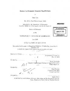
the lost of capital due to depreciation. In such case capital accumulates and the economy displays positive growth. Note that only when ρ > 0, output can be positive even though R may be zero, (Y (K, 0) > 0). In other words, capital and the nonrenewable resource must be substitutes in production, if positive output has to be assured. Hence, a precondition for the prices of nonrenewables to approach inÞnite (q → ∞) is the ability of the economy to accumulate capital and the degree of substitution between K and R. At this point, we would like to pinpoint another contributing aspect of our study. Contrary to what Dasgupta and Heal (1974) propose, here we Þnd that the long run behavior of q does not only depend on whether inputs are substitutes or not in production. In addition to this, the long run behavior of q also depends on the size of the rate of depreciation and the CES share parameter α. In Dasgupta and Heal (1974), σ > 1 always leads the economy to inÞnitely value the nonrenewable in the long-run. We above showed ³ 1 that´for low levels of substitution (i.e., ρ values approach to zero from the right), the condition α ρ < δ holds and the result qq˙ = 0 realizes. Figure 1 below depicts the threshold level. Stability of q(t) for α=0.7 and δ=0.04

0.60

1/ρ

α 1/ρ

0.30

δ =0.04 0.00 0

0.2

0.4

0.6

0.8

1

ρ

Figure 1 Stability of q(t) ´ ³ 1 When α ρ < δ holds, the long run marginal productivity of capital becomes insufficient to compensate for the loss in capital depreciation and hence results diverge from the “general solution”, where resource price grows to inÞnite values. This result also shows that the rate of depreciation plays an important role in the behavior of the nonrenewable resource price. 3.2.

Simulations

The simulations of the CES case reveal valuable information on the time path of the model’s variables under varying elasticity of substitution assumptions. Below, we present the time paths of the rental rate of capital r, resource price q, capital K, and extraction rate R. We assume the following parameter values: s = 0.2, δ = 0.04, α = 0.7, K0 = 50, S0 = 25, and ρ = 13 (⇒ σ = 1.5), or ρ = 0 (⇒ σ = 1), or ρ = − 19 (⇒ σ = .9). Note that when ρ = 13 (⇒ σ = 1.5) we have that 1

the conditions of stability for Case 3 hold (α ρ − δ = 0.545 > 0 and ρ = 13 > 0) and therefore the price of the nonrenewable grows to inÞnity (see Figure 2.b). When ρ = 0 (⇒ σ = 1), and ρ = − 19 (⇒ σ = 0.9) the stability condition of Case 1 holds which refers to the case when q converges to a constant. The rental rate of capital shows a similar behavior in the three cases in the sense that it always converges to a constant (see Figure 2.a). Nonetheless, r converges to different levels, depending on the elasticity of substitution assumption. In particular, when ρ = 13 (⇒ σ = 1.5), r converges to 1

1

r = α ρ , given that α ρ − δ > 0 holds. When ρ = 0 (⇒ σ = 1) or ρ = − 19 (⇒ σ = .9) we observe that

15

r tends to δ. In the former case, the level of r is large enough to compensate for the loss of capital due to depreciation, and hence, capital accumulates and tends to inÞnity as Figure 2.c displays. Otherwise, capital stock tends to zero level after showing some increase initially. The behavior of resource price is substantially affected by the rental rate of capital. When that rate converges to δ, the net return for capital assets become zero, and hence the price of nonrenewable converges to a constant. Otherwise, its price explodes (see Figure 2.b). The extraction R path of the nonrenewable resource tends to zero for any elasticity of substitution assumption; nonetheless, larger levels of extraction are observed in the short run when the resource is a substitute in production. This is optimal as the economy calculates that it may initially exploit resource stocks for accelerating capital accumulation, which can be later used to substitute for the resource as it depletes (see Figure 2.d).

Rental rate of capital r(t) 0.70 0.60 0.50 0.40

σ = 1.5

r 0.30

Cobb-Douglas

0.20 0.10

σ = 0.9

0.00 0

20

40

60

t

80

100

Figure2.a The time path of r(t)

Resource price q(t) 300.00 250.00

σ = 1.5

200.00 q 150.00

Cobb-Douglas

100.00 50.00

σ = 0.9

0.00 0

50

100 t

150

200

Figure 2.b The time path of q(t)

Capital K(t)

σ = 1.5 100 K

Cobb-Douglas

σ = 0.9 0 0

50

100 t

150

Figure 2.c The time path of K(t)

200

16

Resource use R(t) 20

15

σ = 1.5

R 10

Cobb-Douglas

5 σ = 0.9 0 0

10 t

20

Figure 2.d The time path of R(t) 4.

Conclusion

In this paper, inspired by Dasgupta and Heal (1974), we have studied the growth behavior of an economy in the presence of a nonrenewable resource. Like Dasgupta and Heal (1974), we integrated a nonrenewable resource sector with an output sector. In contrast to them, we focused on market solution, as it reveals clearer information on the behavior of variables and on Hotelling’s rule. The basic difference between our model and Dasgupta and Heal’s model, however, is that we differentiate between the rental rate of capital and interest rate, which is used to discount proÞts in the resource sector. This single difference substantially changes the transitional and long-run behavior of the rental rate of capital r and the non-renewable resource price q. This is because the efficiency rule for resource extraction can be expressed as a differential equation in terms of capital-resource extraction ratio, which grows inÞnitely if there is no countervailing factor. We Þrst show analytically that, with a Cobb-Douglas technology, the nonrenewable resource price converges to a constant. Next, we extend our analysis to CES technology using simulations, and show that a similar behavior of resource price is observed if the nonrenewable is a complement. Our simulation analysis also reveals that the elasticity of substitution assumption heavily affects the path of depletion and capital accumulation. We show that for levels of elasticity of substitution close to one from the right the model reproduces results similar to those cases when R is an essential input in production. We conclude that the economy would shrink if elasticity of substitution is not sufficiently greater than one. Our analysis shows that the dynamic general equilibrium version of Hotelling’s rule does not imply an inÞnitely growing resource price. This solves, at least partially, the paradox between the Hotelling’s rule and the empirical evidence that resource prices are constant in the long-run. However, our results are not complete due to at least two reasons, which brings us to suggest two research questions. First, our analysis needs to be extended into Ramsey setup, where the saving/consumption allocation is endogenously made. We believe that the (long-run) results would not change qualitatively. Nevertheless, an endogenous saving/consumption allocation brings into stage an important additional factor in depleting-resource analysis: the consumer’s patience. When it is known that a nonrenewable resource is being depleted, discounting the future plays a crucial role in consumptioninvestment decisions. In that respect, the impact of the consumer’s patience on the optimal depletion of resources must be signiÞcant and deserves investigation. Secondly, we ignored technological improvements in our analysis. However, technological change is the second alternative way of mitigating resource needs and may reduce the demand for nonrenewable resources. Hence, the optimal behavior of resource price depends on technology and

17

technological change. This is the second area that we suggest for future work.

18

References Chiang, A.C. (1992), Elements of Dynamic Optimization, McGraw-Hill, International Editions, Singapore. Dasgupta, P., and Heal, G. (1974), ”The Optimal Depletion of Exhaustible Resources”, Review of Economic Studies (Symposium on the economics of exhaustible resources), 41, 3-28. Gordon, R.L. (1967), ”A Reinterpretation of the Pure Theory of Exhaustion”, The Journal of Political Economy, 75, 274-86. Gray, L.C. (1914), ”Rent under the Assumption of Exhaustibility”, Quarterly Journal of Economics, 28, 66-89. HerÞndahl, O.C. (1955), ”Some Fundamentals of Mineral Economics”, Land Economics, 31, 131-38. Hotelling, H. (1931), ”The Economics of Exhaustible Resources”, Journal of Political Economy, 39, 137-75. Kay, J.A. and Mirrlees, J.A. (1975) ”The Desirability of Natural Resource Depletion”, In The Economics of Natural Resource Depletion (Ed. D.W. Pearce and J. Rose), pp.140-76. New York: John Wiley. Krautkraemer, J.A. (1998), ”Nonrenewable Resource Scarcity”, Journal of Economic Literature, 36 (4), 2065-2107. Peterson, F.M. and Fisher, A.C. (1977) ”The Exploitation of Extractive Resources A Survey”, The Economic Journal, Vol.87, pp.681-721. Smith, Vernon L. (1968) ”Economics of Production from Natural Resources”, The American Economic Review, Vol.58 (3), pp.409-31. Solow, R. M. (1956). ”A Contribution to the Theory of Economic Growth.” Quarterly Journal of Economics, Vol. 70, No. 1 (February) 65-94. Solow, R.M. (1974), ”Intergenerational Equity and Exhaustible Resources”, Review of Economic Studies (Symposium on the economics of exhaustible resources), 41, 29-45. Stiglitz, J.E. (1974a), ”Growth with Exhaustible Natural Resources: Efficient and Optimal Growth Paths”, Review of Economic Studies (Symposium on the economics of exhaustible resources), 41, 123-37. Stiglitz, J.E. (1974b), ”Growth with Exhaustible Natural Resources: The Competitive Economy”, Review of Economic Studies (Symposium on the economics of exhaustible resources), 41, 139-52. Stiglitz, J.E. (1976), ”Monopoly and the Rate of Extraction of Exhaustible Resources”, American Economic Review, 66(4), 655-61. Sweeney, J.L. (1977), ”Economics of Depletable Resources: Market Forces and Intertemporal Bias”, Review of Economic Studies, 44, 125-42. Weinstein, M.C. and Zeckhauser, R.J. (1975) ”The Optimal Consumption of Depletable Natural Resources”, The Quarterly Journal of Economics, Vol.89 (3), pp.371-92.

19

Appendix A ³ ´ K0 Here we show that q (0) = 1−α α−s S0 . Note that the resource constraint that the total amount ¢ ¡R ∞ of extractions 0 R (t) dt must equal the initial stock of the non-renewable S0 can be rewritten as Z

∞

0

Since r = Z

∞

1−α R (t) dt = α ³

αα (1−α)1−α q 1−α

q (t)

´1

α

e

0

0

α

∞

0

Rt s r (q) K0 e 0 ( α r(τ )−δ)dτ dt = S0 q

and by

R t ³ s ³ q˙

1 −α

Z

q

q˙ q

´ ´ +δ −δ dτ

(59)

= r − δ (59) can be rewritten as

dt =

S0 (1 − α) K0 1

(60)

1 α

Note that

e

R t ³ s ³ q˙ 0

α

q

´ ´ +δ −δ dτ

Rt

s−α s d ln q 0 α dτ dτ + α

= e

s

= eα =

µ

(

ln

q(t) + s−α q(0) α

(

q (t) q (0)

¶s

α

)δt

)δt

s−α e( α )δt

(61)

Substituting (61) into (60) we get 1 q (0)

s α

Z

∞

q (t)

s−1 α

s−α e( α )δt dt =

0

S0 K 0 (1 − α) 1

(62)

1 α

Claim Z

∞

q (t)

s−1 α

s−α e( α )δt dt =

0

¯∞ s−α e( α )δt ¯¯ 1−α ¯ (s − α) (1 − α) α ¯ q (t)

s−α α

0

s−α

qssα lim e( =

s−α α

t→∞

)δt − q (0) s−α α

(s − α) (1 − α) =

q (0)

1−α α

s−α α

(α − s) (1 − α)

1−α α

Since this limit must exist we impose that s < α. Proof. It suffices to show that

(63)

20

d

µ

s−α δt s−α α α e 1−α (s−α)(1−α) α

(

q(t)

)

dt

¶

= q (t)

s−1 α

s−α e( α )δt

(64)

Taking the time derivative we get

d

µ

q(t)

s−α α

(s−α)(1−α)

1−α α

s−α e( α )δt

dt

¶

)δt µ s − α q˙ µ s − α ¶ ¶ = + δ 1−α α q α (s − α) (1 − α) α q (t)

q (t)

=

s−α α

s−α α

e(

e(

s−α α

α (1 − α)

q (t)

=

s−α α

s−1 α





)δt  q˙   + δ q  | {z }

1−α α

r

s−α e( α )δt

α (1 − α) = q (t)

s−α α

1−α α



α α

α)  α (1 − 1−α q α

1−α α

 

s−α e( α )δt

(65)

Substituting (63) into (62) we get K0 q (0) = S0

µ

1−α α−s

¶

(66)

Appendix B Firstly, if r → ∞ and ρ > 0 we have that (44) becomes 

1 1−ρ

 1−ρ ρ

 (1 − α)  lim  lim q =  1 r−→∞,ρ>0 r−→∞,ρ>0 α 1−ρ 1− ρ

1

= (1 − α) ρ

(67)

r 1−ρ

that is q would be a constant in the long run contradicting that then applying L’Hôspital’s rule to (44) we have

1

q˙ q

> 0. Now if r → ∞ and ρ < 0

1

1

(1 − α) ρ r α 1−ρ (1 − α) ρ lim q = lim ³ = lim − 1−ρ ³ ρ ´1 ´ ρ 1 r−→∞,ρ